Lean-burn operation for natural gas/air mixtures: the dual-fuel engines

(1)

UNIVERSITA’ DEGLI STUDI DI ROMA

“TOR VERGATA”

FACOLTA’ DI INGEGNERIA MECCANICA

DOTTORATO DI RICERCA IN

INGEGNERIA DELL’ENERGIA-AMBIENTE

XX CICLO

“LEAN-BURN OPERATION FOR NATURAL GAS/AIR

MIXTURES: THE DUAL-FUEL ENGINES”

DOCENTE GUIDA:

PROF. STEFANO CORDINER

COORDINATORE: PROF. FABIO GORI

CANDIDATO:

(2)

i

Abstract

The research activity on internal combustion engines (ICE) is increasingly cast to find an alternative solution to reduce the wide utilization of petroleum fuels like diesel oil and gasoline, for environmental, political and economic concerns.

Natural gas is an ideal fuel to be operated in internal combustion engines, since its characteristics allow for much lower environmental impact (less NOX, PM and PAH emissions) and reduced fuel consumption and CO2 emissions with respect the conventional fuels. It also is particularly suitable to be operated under high volumetric compression ratio engines, thus providing higher efficiency, and moreover it is characterized by a wide flammability range. This latter aspect promotes the employment of a lean burn strategy, thus further increasing the engine efficiency and reducing the exhaust emissions.

The dual-fuel natural gas/diesel concept allows extending the lean flammability limit of NG with respect to SI-NG operations and simultaneously reducing the NOX-PM trade-off affecting diesel combustion. Such a technology consists in introducing NG as main fuel in a conventional diesel engine. A certain amount of diesel pilot injection is preserved to act as the ignition source for the air/NG mixture.

The easiness of dual-fuel conversion, just introducing a feeding system for the NG and optimizing the diesel pilot quantity, makes such technology rather inviting especially as a retrofit for the existing diesel vehicles, which could not meet the more and more stringent emission regulations in the future, thus accelerating the effectiveness of a pollutants reduction strategy, especially in urban areas.

In the present study, the dual-fuel combustion process with its inherent complexity, deriving from the different combustion mechanism of the two fuels (diesel oil and NG), is investigated both from an experimental and a numerical point of view.

The experimental activity has the main target to analyze the problems connected with the conversion of a heavy-duty diesel engine to dual-fuel operation, and to put into evidence the influence of the main engine parameters on performance and pollutants

(3)

ii

formation. Further devices like throttling, catalyst and EGR have been subsequently analyzed to further reduce the exhaust emissions.

The numerical activity, characterized by a mixed 1-D/3-D approach, has been carried out with the initial target of a correct understanding of the complex dual-fuel combustion mechanism. A diagnostic approach has been thus followed, to the aim of getting useful information on the combustion progress by means of the analysis of the experimental in-cylinder pressure data. A detailed multi-dimensional simulation of the whole working cycle of the engine has been subsequently performed, to provide for the correct representation of the fluid-dynamic effect involved in dual-fuel operations. Such an approach allows for the complete description of the engine overall behavior and the dual-fuel combustion in detail.

As far as 3-D simulation tools are concerned, the open-source KIVA-3V code has been utilized, and a fair number of mathematical models have been introduced, with respect the KIVA original version, to correctly represent diesel spray processes and overall combustion. In particular, the WAVE model has been utilized to describe both the diesel jet atomization and the droplet breakup process. The Shell model has been introduced to represent the low-temperature chemistry of the diesel fuel, thus allowing for the correct description of the auto-ignition process. Overall combustion has been simulated by means of a flamelet (CFM model) and a characteristic-time (CTC model) approach. A comparison between these strategies has been performed and main assumptions, advantages, limits and results of each of the two models have been put into evidence. The numerical model has been finally validated by the comparison with the experimental data.

A further section has been here reported to suggest another strategy to improve the lean burn operation of NG/air mixtures. Introducing a certain amount of H2 (up to 15÷20% in volume) no modification to the engine has to be introduced, and a higher combustion speed can be obtained, due to the much higher laminar flame speed of H2. Such an advantage could be exploited to extend the lean flammability limit for NG engines without suffering from instability and low efficiency.

(4)

iii

Chapter 1 INTRODUCTION

1.1 Overview and Objectives

Natural gas is used as a fuel for transport applications in many countries around the world, and its use in vehicle applications is growing. Besides displacing imported petroleum fuels, one of the primary benefits of using natural gas as a vehicle fuel is the potential to substantially reduce exhaust emissions of harmful pollutants such as particulate matter (PM) and nitrogen oxides (NOX). To maximize the benefits of any natural gas vehicle program, several factors must be considered, including natural gas fuel quality, vehicle engine technology, retrofits versus new vehicles/engines, and safety.

Since the early 1990s, Natural Gas for Vehicles (NGV), generally used in compressed form, has attracted renewed interest throughout the world. A number of countries have carried out large-scale development programs. At the national scale, tax incentives have been implemented to promote the use of this motor fuel. For the time being, the world market of natural gas vehicles remains small and heavily concentrated: over half of the world fleet is located in the Americas, mainly in Argentina and Brazil (Table 1.1). According to the Natural Gas Vehicle Coalition, at the beginning of 2006 there were about 130,000 Natural Gas Vehicles (NGV) on the road in the United States, and more than 4 million worldwide. In Europe to date, the market has only developed to a very small extent. At the instigation of European authorities, this situation seems about to change. The European Commission has set an indicative target: NGV is to represent 10% of transport energy consumption by 2020. The first country to use NGV to a significant

(8)

2

extent, Italy is currently Europe's largest market and represents more than 380,000 vehicles. Possessing natural gas resources, Italy began building up its fleet long ago.

Table 1. 1 NGV worldwide in 2006

In recent years, technology has improved allowing a proliferation of natural gas vehicles, in particular for vehicle fleets, such as taxicabs and public buses. Nowadays, virtually all types of natural gas fuelled vehicles may be found either in production for sale to the public or under development, from passenger cars, trucks, buses, vans, and even heavy-duty utility vehicles. Today, most of the heavy gas-powered vehicles are buses and refuse collection vehicles. These applications are especially appropriate for use in urban areas, for a number of reasons. They generate low levels of noise and polluting emissions. In a city, it is not a problem if a vehicle has a limited range or onboard fuel

(9)

3

storage capacity. Finally, with respect to logistics, there is a concentration (compressors) at the depot.

In light vehicles, natural gas can be used in bi-fuel vehicles (gasoline/NGV) or in vehicles running exclusively on natural gas. The intrinsic properties of natural gas are best exploited in dedicated vehicles. Nevertheless, the problem is that the motorist needs access to a widespread NGV distribution network. There are few NGV service stations in existence today, which is why carmakers have generally included bi-fuel (gasoline/NGV) rather than dedicated models in their vehicle range.

A country or region’s current pattern of fuel usage is also important when evaluating the potential benefits of a natural gas vehicle program. For example, Brazil currently produces significant amounts of ethanol from domestically grown sugar cane for use as a vehicle fuel, primarily in light-duty cars. Anyway, it is highly dependent on imported petroleum to supply diesel fuel for heavy-duty vehicles. At the same time, Brazil’s natural gas production ranks fifth in Latin America and recent discoveries suggest that the potential exists to increase production substantially. Brazil is also a highly urbanized country, with significant transportation related air quality problems in its major cities. As such, Brazil could potentially reap significant environmental, public health, and economic benefits from increasing its use of domestic natural gas reserves for transportation. A significant portion of Brazil’s light-duty fleet already runs on domestically produced ethanol. The criteria pollutant emission reductions that can be achieved by switching from gasoline or ethanol to natural gas are also generally modest. Therefore, the greatest potential benefit from additional natural gas usage in Brazil’s transportation sector will accrue by focusing on heavy-duty buses and trucks that currently operate on diesel fuel.

Also, the increasing demand of higher engine efficiency and the need to reduce fuel consumption and meet the more and more stringent emission regulations lead to a deep investigation to make maximum use of the high potential of natural gas. Thus, technical solutions as the utilization of lean and ultra-lean NG/air mixture are widely studied. To efficiently burn a very lean mixture of natural gas and air, a much higher and widespread ignition source as to be provided rather than of having a localized spark-plug, and such an

(10)

4

enhancement can be obtained thanks to the combustion of a certain amount of diesel fuel injected into the cylinder.

According to the previous considerations, the Natural Gas/Diesel Dual-Fuel Engines can represent an interesting and useful solution to further spread the utilization of natural gas as the main fuel in the transportation field, thus reducing the dependence on imported petroleum, and to extend the lean limits of NG utilization. Such an approach could be successfully carried out as a new technology, but its proper strength consist in a powerful retrofit approach for the existing diesel engines which could not meet the increasing emission regulations in the future and could be easily, rapidly and at low-cost converted to dual-fuel operation.

Nevertheless, the dual-fuel technology is extremely complex, since two fuels characterized by different combustion processes are simultaneously burned within the cylinder. This study has the main target to investigate the dual-fuel conversion of a heavy-duty diesel engine and to analyze such a complicated combustion mechanism by means of a general (1-D) and detailed (3-D) numerical approach. The numerical results will be validated on the experimental data and discussed.

1.2 Natural Gas Engine Technology

1.2.1 Natural Gas Properties

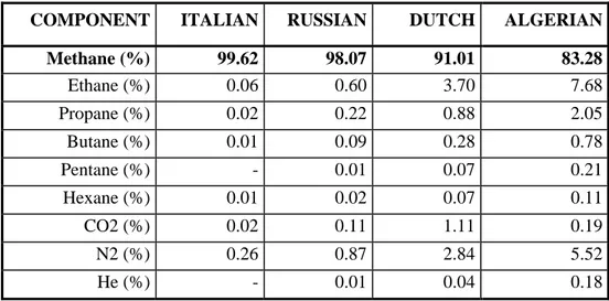
Natural gas is commonly considered as the most inviting short-term fuel alternative for internal combustion engines applications. It should not be referred as an “alternative fuel” anymore, but its wide diffusion is not still satisfactory in comparison with its significant potential to ensure oil-like performance and reduced exhaust emissions. It also is largely available and characterized by low costs with respect to diesel fuel and gasoline. Natural gas is mostly composed by methane, even though its exact composition depends on its provenance, as can be observed in Table 1.2 [1].

(11)

5

COMPONENT ITALIAN RUSSIAN DUTCH ALGERIAN

Methane (%) 99.62 98.07 91.01 83.28 Ethane (%) 0.06 0.60 3.70 7.68 Propane (%) 0.02 0.22 0.88 2.05 Butane (%) 0.01 0.09 0.28 0.78 Pentane (%) - 0.01 0.07 0.21 Hexane (%) 0.01 0.02 0.07 0.11 CO2 (%) 0.02 0.11 1.11 0.19 N2 (%) 0.26 0.87 2.84 5.52 He (%) - 0.01 0.04 0.18

Table 1. 2 Natural gas distributed in Italy

Accordingly, the high potential of NG is referable to the remarkable chemical and physical properties of methane (Table 1.3). It is characterized by a high octane number (RON 120-130) and particularly suitable to be operated in high compression ratio engines, thus leading to high engine efficiency.

METHANE PHYSICAL PROPERTIES

Density (kg/Nm3) 0.72 Flammability Limits (% on air in volume) 5 ÷ 15 Auto-Ignition Temperature (°C) 540

Lower Heating Value (LHV) (MJ/kg) 50.0

Research Octane Number (NOR) 120 ÷ 130

Stoichiometric Air/Fuel Ratio (AFR) 17.2 Table 1. 3 Methane physical properties

Methane, the major component in natural gas, is generally believed to be the cleanest burning hydrocarbon as it produces less CO2 and more H2O than other fossil fuels because of its high H/C ratio. Another important aspect of methane combustion which contributed to its pristine image is the fact that its premixed flames with air do not soot, instead they are blown-out first because of flammability limit considerations. Furthermore, the formation of Polycyclic Aromatic Hydrocarbons (PAH) is widely reduced and a lower flame temperature limits NOX emissions. With respect to gasoline

(12)

6

engines, reduced (-20%) emission of CO2 can be obtained, as well as savings of at least 50% in the fuel cost per km. With respect to diesel engines it is possible to obtain reduced PM and NOX emissions and savings of at least 30% in the fuel cost per km.

From a safety perspective, unlike diesel and gasoline engines, CNG is typically stored in gaseous form under high pressure (at 150 bar or more on light-duty vehicles and at 200 or more on heavy-duty vehicles). These elevated pressures can pose a significant hazard in the event of a valve or tank failure. Nevertheless, because natural gas is lighter than air, gas leaking in the open air will quickly rise and dissipate in the atmosphere to the point that there is no longer a danger of fire or explosion.

Despite of its significant characteristics, the wide diffusion on natural gas is limited by distribution and storage concerns, therefore it has been only partially introduced in the transportation field.

The major problem is represented by the low fuel autonomy. When stored in a vehicle, CNG provides about 1/4 the energy density of gasoline. The range of a CNG vehicle depends on the capacity to store fuel, but generally it is less than (about one-half) that of gasoline-fueled vehicles. Such an aspect obviously affects the design of NG engines, and a mixed gasoline/NG configuration is usually preferred from engine manufacturers, which is not able to properly exploit NG potential yet.Emerging methods of NG storage include Liquefied Natural Gas (LNG), which is already in commercial operation and Adsorbed Natural Gas (ANG), which is still in the developmental stage.

1.2.2 The Lean-Burn Concept

The wide flammability range of natural gas allows regular combustion for very lean mixtures with respect to gasoline engines, thus resulting in high efficiency (low specific fuel consumption) and low NOX emissions. Moreover the utilization of lean mixtures, thus reducing brake torque, can be considered as a useful method to control the engine load without throttling, so minimizing the pumping losses.

The actual drawback is the reduction of the burning rate, mainly due to the lower flame speed, which results in an increase in combustion duration. Once the lean flammability limit is exceeded, the engine stability is affected by cyclic variation, the

(13)

7

engine performance drastically drop and the rapid increase in CO and HC emissions can be observed. Anyway it is still possible to fast and efficiently burn very lean mixtures, even though additional conditions have to be created as high turbulence, turbo-charging or high compression ratio as well (Figure 1.1).

Figure 1. 1 Influence of CR on flammability limits

Table 1.4 shows the performance of a Fiat Mini-Van equipped with different engines [2]. The lean-burn approach allows operating with higher compression ratio and provides higher efficiency. This leads to performance comparable or even superior to diesel and gasoline ones, while reducing CO2 emissions (Figure 1.2). Moreover, NOX emissions can be sufficiently reduced to respect EURO 4 limits by the only use of EGR.

FUEL DIESEL GASOLINE CNG (λ=1) CNG LB

Displacement (l) 2.2 1.8 1.6 1.9

Compression Ratio 18.5 10.5 12.5 14.5

Turbocharging Yes No No Yes

Power (kW @ rpm) 92 @ 4000 92 @ 5600 71 @ 5800 100 @ 4000 Torque (Nm @ rpm) 280 @ 1500 170 @ 3800 145 @ 4000 300 @ 2000

(14)

Chapter 1 INTRODUCTION 8 0 25 50 75 100 125 150 175 200 225 Diesel Gasoline CNG CNG LB CO 2 e m issi o n s [ g /k m ]

Figure 1. 2 Comparison among different fuelling configuration for a Fiat Mini-Van

As already stated, one possible solution to extend the lean flammability limit for natural gas application is to design more sophisticated high-turbulence level combustion chambers [3]. A well-known and successful approach is the “Partially Stratified-Charge” (PSC) concept, proposed by Evans et al. [4]. It consists of introducing an ultra-lean mixture (beyond the lean flammability limit) of air and NG within the cylinder. This main NG injection is then followed by a secondary NG direct injection, localized close the spark-plug, just before the spark timing. It is commonly known that the early stage of the flame growth (the development of the flame kernel) widely influences the overall combustion. To stabilize the whole process, a local enrichment of the mixture close the spark-plug can be provided (Figure 1.3).

(15)

9

Results on PSC test show an improved behavior of the engine up to λ = 1.7, while a homogeneous approach cannot ensure a regular combustion beyond λ = 1.6, as can be observed in Figure 1.4. 2 2.5 3 3.5 4 4.5 5 5.5 6 1.35 1.4 1.45 1.5 1.55 1.6 1.65 1.7 1.75 λ

Brake Power [kWa]

homogeneous PSC 200 210 220 230 240 250 260 270 280 1.35 1.4 1.45 1.5 1.55 1.6 1.65 1.7 1.75 λ BSFC [g/kWh] homogeneous PSC

Figure 1. 4 Comparison between homogeneous and PSC operation

A further interesting solution is to feed the engine with an ultra-lean homogeneous NG/air mixture while enhancing the needed energy for the ignition and the regular development of the flame. As an example, a certain amount of diesel oil can be injected into the cylinder near the TDC. Its combustion provides the ignition source for the homogeneous mixture, thus leading to the presence of a large number of ignition points within the combustion chamber, instead of having a localized spark-plug. Such a technology is usually referred as “Dual-Fuel”.

1.2.3 The Natural Gas/Diesel Dual-Fuel Engine

Diesel/NG dual-fuel engines are one of the possible short-term solution to reduce emissions from traditional diesel engines (affected by the PM-NOX trade-off) meanwhile utilizing an “alternative fuel” like natural gas as primary fuel. It consequently results in an interesting technology to meet future emissions regulations, but also a powerful solution to retrofit existing engines, so longing their life with consistently reduced global environmental impact.

In a dual-fuel natural gas/diesel engine the primary fuel (NG) is mixed with air in the intake manifold, just like a SI engine. The mixture is then compressed and

(16)

10

subsequently ignited by the combustion of a small amount of diesel fuel (the pilot), injected as the piston approaches the top dead centre (Figure 1.5).

Figure 1. 5 Dual-Fuel technology

The wide zone of ignition, due to the presence of a large number of flame kernels in the chamber (Figure 1.6) instead of a localized spark plug, leads to a regular combustion of the whole charge into the cylinder also for very lean mixtures, thus extending the operating flammability limits of natural gas with respect to a spark-ignition solution.

Figure 1. 6 A schematization of the “multi-point ignition” phenomenon

The use of very lean mixtures, together with the high octane number (NOR = 130) of the natural gas, also allows to prevent the occurrence of knock. Accordingly, the use of natural gas as primary fuel allows keeping the original compression ratio of the conventional diesel engine. Thus, the existing and already running on-road diesel engines can be easily converted to dual-fuel operation. In fact the only equipments that have to be

(17)

11

installed on the engine are the feeding system for the NG and the external device allowing to vary diesel injection flow rate. This results in great capital cost and time saving in comparison with other environmental low-impact solutions (fuel cells, hybrid vehicles).

A relevant aspect that has to be considered is the interaction between diesel oil and NG combustion, since they are characterized by different mechanisms. Karim et al. [6] schematized dual-fuel combustion as consisting of three main phases (Figure 1.7):

I. Energy released from diesel combustion;

II. Energy released from combustion of natural gas surrounding diesel flames; III. Energy released from combustion of overall natural gas.

Figure 1. 7 Schematization of dual-fuel combustion

Accordingly, the correct propagation of the flame throughout the homogeneous mixture widely depends on the load, that is to say on the air/NG equivalence ratio. For too lean mixtures, the flame cannot completely propagate and only the natural gas in the vicinity of the diesel flames burns. When the mixture becomes richer, a more regular flame propagation is detected.

(18)

12

It is anyway complicated to establish the correct lean flammability limit in dual-fuel combustion. In fact, it is very similar to the PSC Concept, considering that the combustion of the diesel pilot locally reduces the air available for NG oxidation. Thus, the air/NG equivalence ratio near the diesel flames could be even close to the stoichiometric value. Moreover a large number of flames are expected to interact and join within the cylinder, and then a shorter path has to be covered by each flame.

1.2.4 Dual-Fuel Features and Strategies

Dual-fuel pilot-injected natural gas/diesel engines have a significant potential to reduce NOX and PM emissions from the baseline diesel case, as shown from Papagiannakis and Hountalas [7] (Figure 1.8). Particulate emissions can be decreased with the substitution of a large amount of oil with NG. Moreover, the combustion of a homogeneous lean charge minimizes the local peaks of temperature and thus NOX concentration in the exhaust gases.

Figure 1. 8 Effect of NG percentage on soot and NOX formation

Lower values of the fuel specific consumption and the low atomic ratio C/H of NG (mostly composed by methane) allow the reduction of CO2 emissions, not yet ruled but considered as one of the most important cause of the greenhouse effect).

(19)

13

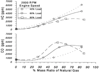
In the recent years the dual-fuel combustion system has been proposed [8-11], but has not reached a great diffusion. This can be explained considering that HC and CO emissions from a dual-fuel engine are higher than those of a conventional diesel engine, especially at part loads (Figure 1.9).

Dual-fuel engines, deriving from the conversion of conventional diesel engines, usually operate unthrottled, with the load regulated by the admission of natural gas in the intake manifold. The air-fuel mixture becomes leaner as the load is reduced, thus approaching the lean flammability limit of the mixture. The consequent combustion process is slow and this leads to the formation of incomplete combustion products (CO) and unburned hydrocarbons (HC). The increase in CO emissions is also due to the local mixture enrichment because the injected diesel pilot mixes with a carburated NG/air mixture instead of just air as in a conventional diesel engine.

Figure 1. 9 Effect of NG percentage on HC and CO formation

Moreover other sources for high HC exhaust emissions are the scavenging phase and the crevice volumes. Unlike a conventional diesel engine, for dual-fuel operations the charge entering in the cylinder through the inlet valve is a mixture of air and natural gas: thus a fraction of the gaseous fuel is forced into crevice volumes during the compression stroke or escapes through the exhaust valve during the valve overlap period (usually

(20)

14

referred as “short-circuit effect”). This last aspect is particularly relevant when the overlap is great, as it is usual for turbo-charged diesel engines.

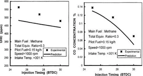
The low efficiency and the high emissions under part loads represent, together with the occurrence of knock at high loads (unavoidable for mixtures near to stoichiometric conditions), the major problems for the traditional dual-fuel conversions. Many possible solutions have been studied to improve the behavior of dual-fuel engines under part loads. A possible approach is the optimization of the pilot injection characteristics [12,13]: increasing pilot quantity and advancing injection timing a more regular combustion process can be observed, with higher efficiency and lower HC and CO emissions (Figures 1.10 and 1.11).

Figure 1. 10 Effect of the pilot quantity on HC and CO emissions

(21)

15

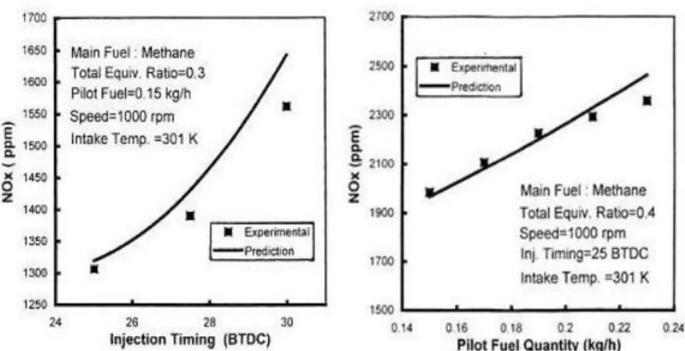
Nevertheless these solutions can be responsible of an increase in NOX emissions (Figure 1.12).

Figure 1. 12 Effect of the pilot quantity and injection timing on NOX emissions

Another possible approach consists in reducing the amount of air and NG in the cylinder, by the introduction of intake throttling or varying intake valve timing. Nevertheless, these solutions can give high PM, CO and NOX emissions. Recent studies [14] show that the use of low pilot quantities (about 2-3%), together with advanced pilot injection (45-60 CAD BTDC), permits to obtain very low NOX emissions and "diesel-like" performance.

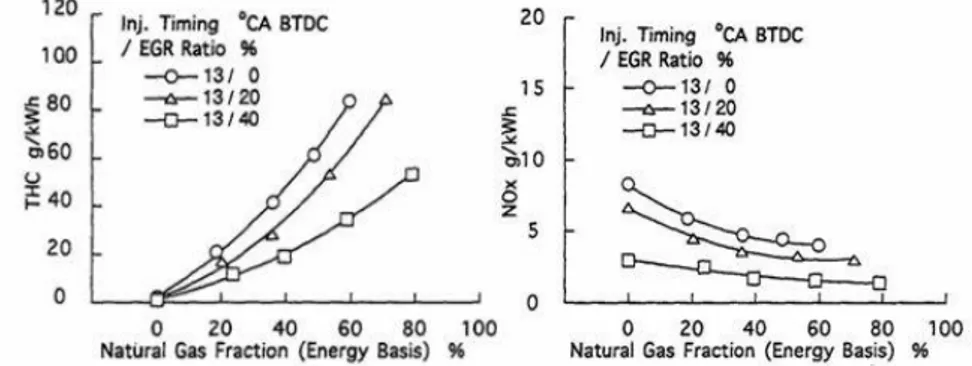
Daisho et al. [15,16] have carried out engine tests modifying some engine parameters as pilot injection timing advance, intake throttling and hot and cooled EGR (Figure 1.13). It was found that hot EGR is the best way to increase thermal efficiency and simultaneously reduce HC and NOX emissions (Figure 1.14). With advanced injection timing a better thermal efficiency can be obtained, however NOX emissions result to be higher (Figure 1.15). Intake throttling promotes better combustion, nevertheless increasing pumping losses.

(22)

16 Figure 1. 13 Comparison among different solutions to improve part-load dual-fuel behavior

Figure 1. 14 Effect of EGR on HC and NOX

(23)

Chapter 2 THE NUMERICAL APPROACH

17

Chapter 2 THE NUMERICAL APPROACH

2.1 Modeling Turbulent Combustion

2.1.1 Turbulent Scales

A turbulent flow consists of large number of vortical structures of different sizes. The size of the largest vortices usually scales with the flow dimensions whereas the size of the smallest structures (Kolmogorov eddies) depends on the Reynolds number and decreases as the Reynolds number increases. The interaction between structures of different dimensions is best explained by the energy cascade concept [17]. It states that the kinetic energy produced by the velocity gradients is transferred from the large to smaller and smaller scales by an inviscid process down to the smallest scales where the energy is dissipated into heat (at the molecular level) by means of viscous motion.

The size of the large turbulence eddies can be calculated by the following expression:

∫

∞ =

0 R dx

L_I _x (2.1)

LI is also called integral length scale of turbulence, whereas RX is the correlation coefficient, varying in the range of 0 to 1.

(24)

Chapter 2 THE NUMERICAL APPROACH 18 4 3 T 4 1 3 Re − = ⎟ ⎠ ⎞ ⎜ ⎝ ⎛ = _I k L L

ε

ν

_(2.2)

where ν is the kinematic viscosity and ε is the kinetic energy dissipation rate. It is defined using Kolmogorov hypothesis and it is strictly related to the concept of the energy cascade of the turbulent spectrum.

An intermediate length scale is the Taylor micro-scale LM which is defined based on the velocity gradients as follows:

(

2 2

)

₀ 2 2 x x x M x R L = ∂ ∂ − = _(2.3)

In addition to the length scales it is possible to define analogous time scales, here neglected since they have similar expressions, apart from dimensional concerns.

2.1.2 Turbulent Combustion Regimes

Under turbulent combustion conditions, the interaction between the turbulent flow field and the flame front is described by means of characteristic dimensionless numbers. The most commonly used are the turbulent Reynolds number (ReT), Damköhler (Da) and Karlovitz number (Ka) defined as:

ν I L u′ = T Re L L I c t s u L δ τ τ ′ = = Da _⎟⎟ ⎠ ⎞ ⎜⎜ ⎝ ⎛ ′ ⎟⎟ ⎠ ⎞ ⎜⎜ ⎝ ⎛ = = k L L k c L u s t t δ Ka (2.4)

The turbulent Reynolds number describes the ratio of the momentum forces (destabilizing effects) to the viscous forces (stabilizing effect). Reacting flows at high turbulence Reynolds numbers are characterized by highly fluctuating flames. The Damköhler number relates the time scale of the turbulent mixing, defined as LI/u’, to the time scale of the chemical reaction defined as δL/sL. When Da >> 1, the chemistry is fast

(25)

19

and the combustion is controlled by mixing processes. The resulting flame front is so thin as it can easily be distinguished and detected. Flame at small Damköhler numbers (Da < 1) are characterized by intense mixing. The reaction of combustion is controlled by chemical kinetics and flames referred to as well-stirred reactor are formed. The Karlovitz number relates the time scale of the chemical reaction (δL/sL) to the smallest time scale of the turbulent flow, represented by the Kolmogorov scale (Lk/u’). Accordingly, it measures the flame front stretch. Using these three characteristic numbers (ReT, Da and Ka), the turbulent premixed flames can be classified into groups (flame regimes), as postulated initially by Borghi [18] and later extended by Peters [19]. An example of Borghi/Peters diagram is shown in Figure 2.1.

Figure 2. 1 The Borghi’s diagram, modified by Peters

The x-axis in Figure 2.1 represents the size of the flame structures by means of the ratio of the integral length scale of turbulence LI to the laminar flame thickness δL. The y-axis represents the ratio of the turbulence intensity u’ to the laminar flame speed sL.

The Borghi’s diagram is represented again in Figure 2.2, together with the respective turbulent flame structures. Wrinkled flame regime is situated below the horizontal line of constant u’/sL = 1. In that zone the laminar flame speed (sL) is higher

(26)

20

than the turbulence intensity (u’). As a result the flame front propagating with the speed sL is able to dump the turbulent fluctuations. The interaction between flame front propagation and the turbulent flow leads to creation of flame front wrinkles. The thickness of the wrinkled flame front is not changed by turbulence because the smallest turbulent structures (Lk) are larger than the laminar flame thickness (δL). Therefore the turbulence does affect the reaction zone and does not alter the chemical kinetics. In other words the interaction between the flame front and the turbulent flow field is purely kinematic (fluid-dynamic). The corrugated regime is situated above the line of constant u’/sL = 1 and below the line of constant Ka = 1. Since u’ is larger than sL the flame front wrinkling of the corrugated flame regime is more intense than in the wrinkled flame regime and additionally the relatively intense turbulence is responsible for creation of “flame pockets” which are detached from the continuous flame sheet. The Kolmogorov eddies are still not able to penetrate the reaction zone because they are too big (δL < Lk).

(27)

21

In the regimes presented above the reaction layer is not disturbed by turbulence because δL < Lk. Therefore the chemical kinetics can be described by the laminar flame properties (δL, sL). Furthermore this offers a possibility to describe the turbulent flame in a simplified way where the turbulent flame front consists of laminar flamelets embedded in a turbulent flow. This simplification is the classical flamelet concept which is commonly used in modeling of turbulent premixed combustion. The well-stirred rector regime is characterized by Da << 1. Accordingly, the mixing time scale is much shorter than the chemical time scale and thus the combustion process is controlled by chemical kinetics. The intense mixing causes perfect mixing of the combustion products with reactants. As a consequence a classical flame front does not exist anymore, since there is no thin reaction where the combustion takes place. The intermediate distributed reactions regime is still characterized by the presence of a distinguishable flame front. Nevertheless, the Kolmogorov eddies are now able to penetrate the reaction zone and the latter results not so thin as to assume laminar flame properties to describe chemical reactions .

2.1.3 Turbulent Combustion Models

The Favre averaged system of equations describing turbulent flows, is generally expressed as follows: Conservation of Mass 0 ~ = ∂ ∂ + ∂ ∂ α α ρ ρ x u t (2.5) Conservation of Momentum

(

α β

)

α α β αβ α β α β α _ρ τ _ρ _ρ ρ u u x g x x p x u u t u _′′ _′′ ∂ ∂ − + ∂ ∂ + ∂ ∂ − = ∂ ∂ + ∂ ∂ ~ _~ ~ (2.6)

(28)

Chapter 2 THE NUMERICAL APPROACH 22 Conservation of Energy

(

u T

)

x c q m h t p J x x T u t T c r p n i i i T p ′′ ′′ ∂ ∂ − − − ∂ ∂ + ∂ ∂ − = ⎟⎟ ⎠ ⎞ ⎜⎜ ⎝ ⎛ ∂ ∂ + ∂ ∂

_∑

= α α α α α α ρ ρ ρ 0 , ~ ~ ~ & (2.7)

Conservation of chemical species

(

i

)

i i i i Y u x m J x x Y u t Y _′′ _′′ ∂ ∂ − + ∂ ∂ − = ∂ ∂ + ∂ ∂ α α α α α α ρ ρ ρ ~ ~ ~ _, _& i=1, n (2.8)

Equation of State (Perfect Gas)

(

)

I T

R

p=ρ ~= γ −1ρ~ I = cvT (2.9)

It is unclosed, due to the presence of two kinds of unknown terms. The first one is represented by the terms deriving from the mean operation of the product between two favre fluctuations

(

ρu_α′′u_β′′, ρu_α′′T′′, ρu_α′′Y_i′′

)

. Such terms have to be solved by the introduction of a proper turbulence model. Secondly, additional unknown quantities, m&i

and

∑

= n i i im h 0

& , derive from the presence of chemical reactions within the flow and cannot be represented by Arrhenius-type laws in a turbulent flow. Thus, the introduction of a proper combustion model is needed.

A turbulent combustion model calculates the reaction rate,

[ ]

t

∂

=

m

_i

ω

_&

, which represent the rate of conversion of the generic chemical species. Since last years, several mathematical models have been introduced to describe the combustion process. A list and a brief description of them are here below reported:

The Zimont Model, which describes the combustion process in terms of a single transport equation for a progress variable “c”. The transport equation is

(29)

23

closed using a model to calculate the turbulent flame speed (sT), derived using physically justified simplifications and dimensional analysis.

The Eddy-Break-Up (EBU) Model, developed by Spalding [20], which calculates the mean reaction rate as only function of the turbulent quantities k (kinetic energy) and ε (kinetic energy dissipation rate). It was further developed by Magnussen e Hjertager [21] and referred to as Eddy-Dissipation

Model.

The Abraham Model [22], developed on the basis of EBU model, which calculates the mean reaction rate while taking into account for chemical reactions too. It is also commonly known as Characteristic-Time Combustion

(CTC) Model.

The Bray-Moss-Libby (BML) Model [23], which first introduces the two-zone hypothesis. The combustion chamber is divided into two separate regions (burned and unburned zone) by means of a flame front, which results to be so thin to assume laminar properties to model chemical reactions. The flame is corrugated by the action of the largest eddies but the smallest eddies cannot penetrate the flame (Ka < 1). Such a hypotesis follows the flamelet approach (Figure 2.2), that is why the BML model can be considered as the real ancestor of the flamelet models. It was further developed by Cant-AbuOrf [24] which introduced the progress variable “c” to describe the combustion process.

The flamelet models, which follow the BML assumptions and describe the kinematic evolution of the flame front (Coherent Flame Model) or are based on a level set approach (G-equation Model).

(30)

24

The Pdf Models, characterized by a statistical approach and wondering about the probability of the thermo-fluid-dynamic or chemical quantities having a certain value at a certain time, in a certain point of the computational domain.

The Eddy Dissipation Concept (EDC) Model, assuming part of the fluid to be thoroughly mixed within a particular cell as well as to be the main driver for chemical reaction. These well mixed portions of a sub-volume, the so called “fine scales”, are regarded to resemble a constant pressure reactor. That way the governing equations loose part of their complexity. Using the simplified equations for species conservation the corresponding source terms are derived from an Arrhenius-type reaction mechanism. It is particularly suitable to import detailed kinetic mechanisms.

The proper combustion model has to be chosen on the basis of the particular application field (Table 2.1).

Premixed Flames Diffusive Flames Partially Premixed Flames BML, Cant, CFM (Flamelet) Zimont (Progress variable)

Mixture Fraction Model Progress Variable + Mixture Fraction Fast Chemistry

Eddy Break-Up Model (EBU) Characteristic-Time Combustion (CTC)

Eddy Dissipation Model (EDM)

Finite Chemistry

Eddy Dissipation Concept (EDC) PDF Transport Model

G-Equation Model Table 2. 1 Combustion models and their application field

If chemistry is infinitively fast in comparison with turbulent timescale, a model describing chemistry as a single-step reaction can be usefully considered. In particular, to simulate premixed flames, the flamelet approach is commonly followed. When chemistry is not infinitively fast or a more general model is required rather than the flamelet (i.e. for

(31)

25

the distributed reactions regime), PDF, EDC and G-equation Model are preferred. Such models allow taking into account for detailed kinetic mechanisms.

2.2 Overview on Dual-Fuel Combustion Simulation

First numerical activities on dual-fuel combustion and exhaust emissions, which are available on literature, have been mainly characterized by a multi-zone 0-dimensional (0-D) or quasi-dimensional approach [25-27].

In such studies the combustion chamber is usually divided into a certain number of zones representing the unburned and burned zones, or diesel premixed, diesel diffusive and NG combustion. Within each zone, no gradient of temperature, pressure or species concentration is considered and for the most simplified models no heat exchange between different zones is assumed. Even though such approaches well predict experimental data, they are not properly suitable to completely understand the dual-fuel combustion. Such a process is extremely complex and cannot avoid a locally-performed analysis of the interaction between diesel and natural gas combustion. Moreover the proper flow field has to be taken into account, since it widely influences the whole process, starting from the pilot injection and passing through the mixture formation and ignition up to the overall combustion.

In the last years, due to the improved calculation capability, a multi-dimensional CFD approach has been carried out on dual-fuel engines to analyze the in-cylinder processes.

Basic 3D analyses of dual-fuel combustion are reported in the literature. Reitz et al. [28,29] have used KIVA-3V code to simulate diesel ignition by means of the Shell Model and dual-fuel combustion by the CTC model. It is commonly utilized to describe diesel combustion but has been properly modified to take into account for NG as fuel in addition to oil. They have realized that, when the amount of NG increase (i.e. NG ≥ 90% of the total energy available), the CTC is not able to describe the flame propagation throughout the charge. Therefore they subsequently introduced a G-equation model to simulate overall combustion [30].

(32)

26

2.3 Modeling, Experiments and Interaction

The numerical activity performed during the present study has been mainly based on a multi-dimensional (3-D) approach. This choice is due to the complex phenomena involved in dual-fuel combustion, which is strongly characterized by the local interaction between the main fuel (NG) and its ignition source (the diesel pilot). Moreover, the actual 3-D flow field within the cylinder has to be considered to well describe all the physical processes occurring during a dual-fuel operation (diesel pilot injection, breakup, evaporation, auto-ignition, and overall combustion).

Nevertheless, a preliminary analysis of the behavior of the whole engine (here referred as “diagnostic” strategy) has been carried out by means of a 1-D approach, to get useful information on the dual-fuel combustion process, just having as input the experimental in-cylinder pressure traces. The calculated heat release curves have been then analyzed with the aim to detect and distinguish the single contribution of diesel fuel and NG to the overall combustion. The 1-D approach can also be considered a useful tool to put into evidence fluid-dynamic processes like the “short-circuit effect” and it also has been utilized to provide the correct pressure boundary condition for the subsequent 3-D analysis.

The latter has been carried out by analyzing three fundamental steps (flow field evolution, diesel spray evolution, diesel auto-ignition and overall combustion) and the numerical results have been compared with the experimental ones. Once the model is validated, the predictive approach can be undertaken. The engine key-parameters can be varied, their influence on engine performance can be easily put into evidence, and important guidelines can be provided for the future experimental procedures. In such a way, the interaction loop between experiments and modeling can be finally executed.

The present activity on dual-fuel engines has been performed in the framework of a collaboration between the Univesity of Rome Tor Vergata (UTV) and the Istituto Motori of the Italian National Research Council (IM-CNR), where the experimental tests have been carried out.

(33)

Chapter 3 COMPUTATIONAL TOOLS

27

Chapter 3 COMPUTATIONAL TOOLS

3.1 Analysis of Overall Engine: the FW2001 Code

3.1.1 General Description

The integrated 0-D / 1-D framework FW2001 is an in-house developed code, since it has been entirely developed at UTV. It represents a simple and useful tool to simulate the behavior of the whole engine, from the intake to the exhaust, while being characterized by good predictive ability and reduced calculation time. The overall engine schematization leads to the definition of 0-D and 1-D elements (Figure 3.1).

Figure 3. 1 The real engine and its schematization

Main feature of the 0-D elements is the uniformity of the thermo-fluid-dynamics properties. Accordingly, they are used to model capacities, cylinder-piston and all the elements characterized by uniform thermodynamic properties (Figure 3.2).

(34)

28 Figure 3. 2 0-D elements: an example

0-D elements are modeled as open system allowing the exchange of mass and energy with the external environment. Mass and enthalpy exchanges occur through the permeable sections characterized by flow velocities greater than zero. The study of a 0-D element needs the energy and mass conservation equations, as well as the knowledge of the following quantities:

Volume variation and work

Input and output exchange of mass and enthalpy Heat exchange at the cylinder walls

Chemical Heat Release

Main feature of the 1-D elements is that the thermo-fluid-dynamics properties change along the element main direction, while keeping a constant value along the orthogonal section. Ducts and heat exchangers can be successfully represented by 1-D elements (Figure 3.3). The study of a 1-D element needs the energy, momentum and mass conservation equations.

(35)

29 Figure 3. 3 1-D elements: an example

0-D and 1-D elements are coupled by means of joint elements, which allow for the information exchange between the elements. A coupling can be realized between 1-D elements, or between 0-D elements, as well as between different types of elements. A multiple joint can be realized as well (Figure 3.4).

(36)

30

3.1.2 Solving Method

The sequence of operation that has to be followed is here below reported:

Time-step calculation Crossing section updating Velocity updating

Source terms updating Solution of 0-D joints Solution of 0-D 1-D joints Solution of multiple 1-D joints Solution within 1-D elements 1-D boundary conditions updating Solution within 0-D elements

In such a way the code structure results to be widely flexible. In fact, each element is individually handled and it is possible to utilize different solving methods for the same types of element or joint. Accordingly, more complex algorithm can be used to solve the most critical elements.

The basis equations that describe the mass, momentum and energy balance within the 1-D elements can be expressed in a compact differential form as follows:

0 = + ∂ ∂ + ∂ ∂ S x F t W (3.1) ⎟⎟ ⎟ ⎟ ⎟ ⎟ ⎠ ⎞ ⎜⎜ ⎜ ⎜ ⎜ ⎜ ⎝ ⎛ − + = 1 2 2

γ

ρ

p u u W ⎟ ⎟ ⎟ ⎟ ⎟ ⎟ ⎠ ⎞ ⎜ ⎜ ⎜ ⎜ ⎜ ⎜ ⎝ ⎛ ⎟⎟ ⎠ ⎞ ⎜⎜ ⎝ ⎛ − + + = u kp u p u u F 1 2 2 2 γ ρ ρ ρ ⎟ ⎟ ⎟ ⎠ ⎞ ⎜ ⎜ ⎜ ⎝ ⎛ − + ⎟ ⎟ ⎟ ⎟ ⎟ ⎟ ⎠ ⎞ ⎜ ⎜ ⎜ ⎜ ⎜ ⎜ ⎝ ⎛ ⎟⎟ ⎠ ⎞ ⎜⎜ ⎝ ⎛ − + = q g A dx dA u p u u u S ρ ρ γ γ ρ ρ ρ 0 1 1 2 2 2 (3.2)

where ρ, u, p, γ, A, g, q are respectively density, velocity, pressure, cp/cv ratio, section area, friction coefficient and thermal exchange coefficient. The set of differential

(37)

31

equations is solved through the two-step Lax-Wendroff scheme. This scheme is particularly reliable and describes optimally the propagation of pressure waves within ducts. The 0-D objects are analyzed solving the mass and energy conservation for open systems. The main hypotheses are:

Space uniformity of the thermodynamic variables and the chemical species concentration within the 0-D element

Mass flows incoming in the element instantaneously reach the stagnation conditions

The flow field within the element is everywhere zero

Under these assumptions, the 0-D elements are analyzed through a filling-emptying model, based on the following equations:

0 = −

∑

k k i, k i _X _m dt ) V X ( d & ρ (3.3) * k k k * _m _h _pV Q dt dE ₌ ₊

_∑

₋ & (3.4)

where Xi, m, V*, E, Q* ,hk, are respectively mass fraction, mass, volume variation, energy, heat rate, enthalpy. The joint elements represent the most critical elements of all fluid-dynamics sections. The calculation of the mass and energy fluxes is solved by means of characteristic lines and semi-empirical systems are to account for the loss coefficients. Each joint is characterized by two nodal points, which are connected through calculated loss coefficient. They are fixed through compatibility equations until attainment of the inlet and outlet mass balance. Once obtained mass balance, the objects extremities are fixed by characteristics lines, finding their thermodynamic parameters. The location of loss coefficients is obtained through experimental analysis, which characterizes the dependency on joint geometrical parameters and velocity values.

(38)

32

3.1.3 1-D Approach for Internal Combustion Engines

The proposed 1-D approach allows both predictive and diagnostic analysis of combustion.

A diagnostic approach, based on the heat release calculation can be utilized to analyze the experimental in-cylinder pressure data. To this aim, a single zone model [31], based on the First Law of Thermodynamics, can be used with the following assumptions:

There is no distinction between burned and unburned zones

Cylinder temperature and pressure are assumed to be uniform throughout the combustion chamber

The charge composition does not vary during combustion

The sensible enthalpy from fuel injection is negligible in comparison with the other terms

The contents of the cylinder are modeled as an ideal gas

The effect of the crevice regions, fuel heating and evaporation is negligible

Under the previous assumptions the First Law equation becomes:

wall ghr pdV Vdp dQ dQ + − + − = 1 1 1

γ

(3.5)

where dQghr is the “gross” heat release, dQwall is the wall heat transfer, p is the

measured cylinder pressure, V is the cylinder volume and γ is the ratio of the specific heats of the considered gas. The sum of the first and second terms on the right-hand member is usually referred as “net heat release” too. Heat transfer through cylinder walls is usually modeled by means of semi-empirical correlations:

) ( _g _wall c wall _h _S _T _T dt dQ ₌ ₋ (3.6)

(39)

33

where S is the heat transfer, Tg is the charge temperature and Twall is the wall

temperature. The heat transfer coefficient hc (W/m2K) can be determined by the

Woschni’s correlation [32]: 8 . 0 5 . 0 8 . 0 2 . 0 26 . 3 B p T w h_c = − − (3.7)

where B is the cylinder bore and p, T and w are the cylinder pressure, temperature and mean velocity respectively. Mean velocity is defined as:

) ( 2 1 m rif rif rif d p p p V p T V C S C w= + − _(3.8)

where Sp represents the piston speed, Vd is the volume displaced, pr, Tr and Vr are

the cylinder pressure, temperature and volume at the reference state respectively, p is the cylinder pressure, whereas pm is the cylinder pressure of the corresponding motored

cycle. C1 and C2 constants are expressed as follows:

C1 = 2.28 and C2 = 0 during compression stroke

C1 = 2.28 and C2 = 3.24·10-3 during combustion and expansion stroke

The ratio of the specific heats γ = cp/cv, accordingly with the above assumptions, was considered as a function of the temperature only. The following equations are utilized to describe the dependence from temperature:

)

R

c

(

p p

−

=

γ

(3.9) 12 4 9 3 6 2 10 275 0 10 911 1 10 294 3 1000 337 1 636 3. . T . T . T . T c_p = − + − + (T < 1000 K) (3.10)

(40)

Chapter 3 COMPUTATIONAL TOOLS 34 12 4 9 3 6 2 10 006 0 10 085 0 10 488 0 1000 338 1 045 3. . T . T . T . T cp = + − + − (T > 1000 K) (3.11)

After the diagnostic approach has been carried out, a Wiebe’s functions analysis can be performed to reproduce the calculated heat release rate curves, with the aim to identify the influence of the engine key-parameters on combustion. Secondly, a predictive strategy can be carried out by means of the FW2001. In this case, the numerical code needs the proper input data (a burning mass fraction law) required for the calculation of engine performance. Wiebe’s functions are commonly used in the analysis of the combustion process of diesel engines. The rate of heat released from the combustion of diesel fuel is usually expressed as [33]:

ϑ

d

dQ

d

dQ

d

dQ

₌

p

₊

d (3.12)

(

)

⎥ ⎥ ⎦ ⎤ ⎢ ⎢ ⎣ ⎡ ⎟ ⎟ ⎠ ⎞ ⎜ ⎜ ⎝ ⎛ − − ⎟ ⎟ ⎠ ⎞ ⎜ ⎜ ⎝ ⎛ − + = +1 0 0 ₆₉₀₈ 1 908 6 p p f p f p p p p p . exp f M . d dQ θ θ θ θ θ θ θ ϑ (3.13)

(

)

⎥ ⎥ ⎦ ⎤ ⎢ ⎢ ⎣ ⎡ ⎟⎟ ⎠ ⎞ ⎜⎜ ⎝ ⎛ − − ⎟⎟ ⎠ ⎞ ⎜⎜ ⎝ ⎛ − + = +1 0 0 ₆₉₀₈ 1 908 6 d d f d f d d d d d _. M _f _exp _. d dQ

θ

ϑ

(3.14)

where the index p is referred to the fraction of diesel fuel injected that burns in premixed conditions while the index d is referred to the diffusive phase of combustion. Wiebe’s functions are characterized by the presence of four main parameters, the crank angles duration of combustion θ and _p θ , and the shape factors _d f_p and f_d. M_p and M_d are the amounts of diesel oil that burn under premixed and diffusive conditions respectively. θ0 represents the crank angle at the start of combustion. Typical values for a direct injection diesel engine are [34]:

CAD

7

5

6 ÷

= .

p

θ

m

p

=

3 m

d

=

0.

5

(3.15)

(41)

35

In order to simulate the heat release rate for a dual-fuel engine, a further Wiebe’s function, similar to the previous ones, was introduced for the combustion of natural gas:

(

)

⎥ ⎥ ⎦ ⎤ ⎢ ⎢ ⎣ ⎡ ⎟ ⎟ ⎠ ⎞ ⎜ ⎜ ⎝ ⎛ − − ⎟ ⎟ ⎠ ⎞ ⎜ ⎜ ⎝ ⎛ − + = +1 0 0 ₅ 1 5 gas gas f gas f gas gas gas gas gas exp f M d dQ

θ

ϑ

(3.16)

Accordingly, the eq. 3.12 becomes:

ϑ

d dQ d dQ d dQ d dQ ₌ p ₊ d ₊ gas (3.17)

A typical value for a spark ignition engine is f_gas =2, while θ mainly depends on _gas the equivalence ratio of the air/natural gas mixture. In Figure 3.5, typical heat release rate curves, obtained by means of the Wiebe’s functions, are reported for both (full-diesel and dual-fuel) cases. The standard Wiebe analysis allows to fit the heat release rate curves only for limiting full-diesel and natural gas spark ignition conditions. In dual-fuel modality, Wiebe’s parameters are widely modified by the contemporaneous presence of oil and gas into the combustion chamber.

(42)

36

FW2001 has been successfully used to predict SI engine performance with regard to simple combustion chamber geometries [35-37]. However, when complicated geometries are concerned, a more detailed (3D) approach is desirable to take into proper account non-axial-symmetric chambers. Nevertheless, FW2001 can be successfully used to simulate the presence of the overall engine ducts and devices, in order to provide, starting from the experimental pressure trace, the actual and time dependent boundary conditions to the 3D code, which in turn computes the 3D chamber and intake-exhaust duct fluid dynamics.

3.2 Analysis of In-Cylinder Processes: the KIVA-3V Code

3.2.1 General Description

The multi-dimensional CFD (Computational Fluid-Dynamics) KIVA-3V code, developed at the Los Alamos American National Laboratory, solves the conservation of mass, momentum, energy and species equations for turbulent and reacting flows.

It follows a Finite Volume Method (FVM), and is able to manage structured and moving grids. In this way it is possible to reproduce the real motion of piston and valves. Temporal and spatial differencing is managed by using semi-implicit quasi second order up-winding approaches with the Arbitrary Lagrangian Eulerian (ALE) algorithm. A KIVA’s inviting characteristic is that it is an “open sources” code, which can be modified as the user likes.

The first public release [38] of KIVA was made in 1985 through the American National Energy Software Center, at Argonne National Laboratory, which served at the time as the official distribution center for DOE-sponsored software. The Los Alamos team and other users worldwide soon began testing KIVA in a broad variety of applications. Over time a significant number of papers were presented, each focusing on some aspect of the model and often offering extensions and improvements. The model itself was gradually being made more efficient and realistic, resulting in the public release in 1989 of the improved version previously mentioned, called KIVA-II [39].

(43)

37

KIVA-II extends and enhances the earlier KIVA-II code, improving the computational accuracy and efficiency and its ease of use. The KIVA-II equations and numerical solution procedure are very general and can be applied to laminar or turbulent flows, subsonic or supersonic flows, and single-phase or dispersed two-phase flows. Arbitrary numbers of species and chemical reactions are allowed. A stochastic particle method is used to calculate evaporating liquid sprays, including the effects of droplet collisions and aerodynamic breakups. Although the initial and boundary conditions and mesh generation have been written for internal combustion engine calculations, the logic for these specifications can be easily modified for a variety of other applications.

The KIVA computer program consists of a set of subroutines controlled by a short main program. The general original structure of KIVA-II is illustrated in Figure 3.6, showing a top-to-bottom flow encompassing the entire calculation. Beside each box in the flow diagram appears the name(s) of the primary subroutines(s) responsible for the associated task. In addition to the primary subroutines, Figure 3.6 also identifies a number of supporting subroutines that perform tasks for the primaries.

A cycle is performed in three phases. Phases A and B together constitute a Lagrangian calculation in which computational cells move with the fluid. Phase A is an explicit calculation of spray droplet collision and oscillation/breakup terms and mass and energy source terms due to the chemistry and spray. Phase B calculates in a coupled, implicit fashion the acoustic mode terms (namely the pressure gradient in the momentum equation and velocity dilatation terms in mass and energy equations), the spray momentum source term, and the terms due to diffusion of mass, momentum, and energy. Phase B also calculates the remaining source terms in the turbulence equations. In Phase C (Eulerian calculation), the flow field is frozen and rezoned or remapped onto a new computational mesh.

Such a mixed (Lagrangian - Eulerian) approach allows to well manage moving grid, since the rezone (C) eulerian phase allows to avoid the excessive cell deformation, taking place during the lagrangian phase. Thus, internal combustion engines (characterized by the motion of the piston) can be easily simulated.

(44)

38 Figure 3. 6 General flow diagram for the KIVA program

(45)

39 Figure 3. 6 continued

(46)

40

The two earlier versions of KIVA lend themselves well to confined in-cylinder flows and to a variety of open combustion systems, but they can become quite inefficient to use in complex geometries that contain such features as inlet ports and moving valves, diesel pre-chambers, and entire transfer ports. In these code versions, the entire domain of interest must be encompassed by a single block of computational zones, which may require that a significant number of zones be deactivated.

The latest version of KIVA, known as KIVA-3, is intended to overcome this deficiency [40]. It differs from KIVA-II in that it uses a multi-block structured grid, which allows complex geometries to be modeled with far greater efficiency than KIVA-II, because discrete blocks of zones can now be coupled together to build the required structure. Figure 3.7 shows a computing mesh for a KIVA-3 model of a two-stroke engine.

Figure 3. 7 An example of a multi-block structured grid

The last extended version of KIVA-3, known as KIVA-3V [41], also can model any number of vertical or canted valves in the cylinder head of an internal combustion engine (Figure 3.8). The valves are treated as solid objects that move through the mesh using the familiar "snapper" technique used for piston motion in KIVA-3.

The only difference is that during the piston motion, some planes in the mesh are activated (with the piston moving down) or deactivated (piston moving up). On the contrary, when the valve moves through the mesh, the planes are simply passed from the bottom valve face to the top one (valve moving down) and vice versa.

(47)

41 Figure 3. 8 The introduction of valves in the KIVA-3V version

Because the valve motion is modeled exactly, and the valve shapes are as exact as the grid resolution will allow, the accuracy of the valve model is commensurate with that of the rest of the program.

Other new features in KIVA-3V include a particle-based liquid wall film model, a new sorting subroutine that is linear in the number of nodes and preserves the original storage sequence, a mixing-controlled turbulent combustion model, and an optional RNG k-ε turbulence model. All features and capabilities of the previous KIVA-3 and KIVA-II versions have been retained.

KIVA-3V has been used to successfully model gasoline, diesel and NG fuelled engines since its inception, and still represents the best code to simulate in cylinder processes. Nevertheless, some modifications are needed to improve its predictive capabilities.

Once again, the reader has reminded that the KIVA code is fully open sources. Thus, every subroutine can be easily modified and any sub-model can be directly introduced within the main program. One the contrary, the commercial programs are sold for profit, and the original source code is generally unavailable to the user. What is being marketed is the object code, a “black box” that has been tailored to the user’s requirements, backed up with service and consultation. In contrast to commercial programs, the relatively low cost and ready availability of the source code has created a wide KIVA user community, particularly through the engineering schools and

Lean-burn operation for natural gas/air mixtures: the dual-fuel engines

UNIVERSITA’ DEGLI STUDI DI ROMA

“TOR VERGATA”

FACOLTA’ DI INGEGNERIA MECCANICA

DOTTORATO DI RICERCA IN

INGEGNERIA DELL’ENERGIA-AMBIENTE

“LEAN-BURN OPERATION FOR NATURAL GAS/AIR

MIXTURES: THE DUAL-FUEL ENGINES”

Abstract

Table of Contents

Chapter 1

INTRODUCTION

1.1

Overview and Objectives

1.2

Natural Gas Engine Technology

Chapter 2

THE NUMERICAL APPROACH

2.1

Modeling Turbulent Combustion

∫

ε

ν

(

)

(

)

(

)

∑

(

)

(

)

(

)

∑

[ ]

t

∂

∂

=

=

m

ω

&

&

2.2

Overview on Dual-Fuel Combustion Simulation

2.3

Modeling, Experiments and Interaction

Chapter 3

COMPUTATIONAL TOOLS

3.1

Analysis of Overall Engine: the FW2001 Code

γ

ρ

ρ

ρ

∑

∑

γ

γ

γ

)

R

c

c

(

−

=

γ

ϑ

ϑ

ϑ

d

dQ

d

dQ

d

_∑

_&

_&

_∑

₌

₊