4. INTRODUCTION OF THE INSTRUMENTS 4.1 Introduction

33

4.

INTRODUCTION OF THE INSTRUMENTS

4.1

Introduction

In order to achieve the goals of the assignment some experiments have been conducted with the help of specially designed experimental setup and some state of the art instruments. Because some of the setups/instruments are commonly used by different experiments, they are introduced here in details at one time.

4.2

Keyence Microscope

The Keyence Microscope (Fig. 4.1) is a VHX100 optical microscope [49]. It has been used in the tool stiffness analysis (see Chapter 5) for the tool displacement measurement.

It equipped with:

• three different lenses with different magnification: 50X~175X, 50X~200X, 1000X~3000X; these lens are connected to a colour CCD camera with a built-in illumination, which allows to ensure ideal illumination all the time as well as eliminate illumination setting;

• a five-axis stand where the aforementioned camera can be tilted at any angle and the stage can be rotated by 360°;

• a controller directly linked with the lenses by an optical fibre cable. The controller is equipped with:

o a 15-inch, high-resolution LCD monitor with 1600x1200 pixels. That allows to detect the measurement directly on the monitor;

o a hard disk drive built into which up to 200.000 images can be stored in;

34 During the tool stiffness experiments, the microscope configuration enables the measurement of the position of the wire placed on the tool tip, the displacement at the tool tip and the position of the tool in the clamping system.

The resolution of the microscope depends on the pixel of the monitor and the magnification of the lenses used.

4.3

Keyence Laser Sensor

This instrument has been used for both the static stiffness experiments and the geometric accuracy tests. Its features are [see Appendix C]:

• resolution of 0,01µm; • 12µm diameter beam spot; • 50kHz sampling rate;

• measuring range: 10mm ±0,5mm

The LC Series uses a triangulation measurement system making it one of the most accurate laser displacement metres. If the front surface of the sensor is not perfectly parallel to the target surface, it is possible to compensate an angular error of ±10°.

In Tab. 4.1 is listed the specification of the Keyence laser sensor.

The sensor used during the tests was the LC 2420 (Fig. 4.2) [50]. It has been possible to mount it on a simple fixture.

Fig. 4.2-LC2420 Keyence laser sensor[49]

In Appendix C it is possible to see the trend of the spot diameter as a function of the distance from the centre of the measuring range.

35 Tab. 4.1-Specification of the LC series[53]

4.4

Automation 3200

This software is directly integrated with the machine axis control system, and it has been used during the dynamic accuracy test.

The Automation 3200 contains several utility programs that may be referred or run by commands [53]:

• Nstat: Status / diagnostic screen, view the controller status in a graphical format;

• Nscope: Data collection and plotting (1D or 2D), autotune the axes servo loops and

graphically plot their performance;

• Nplot: Data collection and plotting (3D), continuous plotting of 3 axes of motion during a

CNC program;

36 • Ndebug: Low level command line debug utility, test and monitor the controller's operation.

The Automation 3200 programming language is based on a particular one often referred to as G-Code language. However, the Automation 3200 has many English extended commands, whose syntax is based on simple words, while the G-Code syntax counts the commands insertion through the employment of letters and numbers put side by side. The two different syntaxes can be used together in the same program, as shown below.

This software allows deciding whether to use the rate-based parameters to define the acceleration rate, in distance units/sec2, for “rapid” (point-to-point) and asynchronous motion, or to use the AccelTimeSecAxis parameter to define the time, in seconds, for time-based ramping of “rapid” (point-to-point) moves and asynchronous moves. Moreover it allows setting the type of axis both linear and rotational.

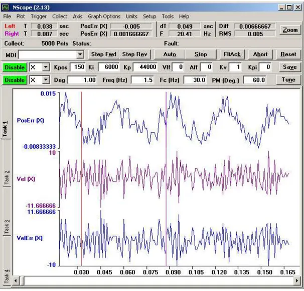
In particular for this work it has been used the Automation 3200’s utility program Nscope, which allows a single step or continuous cycle motion command to be generated for an axis. This can be used to simulate a typical move profile for the users’ desired application allowing the response of the axis to be graphically displayed and adjusted accordingly. Many items can be plotted for each axis; Fig. 4.3 shows an example of the plot of position error, velocity command and velocity error.