4 Three-dimensional seismic structure of Lesser Antilles region

4 Three-dimensional seismic structure of Lesser

Antilles region

4.1 SIMULPS14 in the 3-D simultaneous inversion

In the third step of LET, the 1-D minimum model and the phases of the well-located seismic events selected must be supplied to SIMULPS14. This 3-D inversion program may either invert Tp travel times to constrain a Vp structure, or both Tp travel times and Tp-Ts times to get images of Vp/Vs anomalies. The norm of the misfit function is computed in a damped least squares sense. In order to reduce the inverse problem to a tractable size, it is advisable to use the parameter separation (Pavlis et Booker, 1980) is employed. The grid approach of SIMULPS14 utilizes a linear interpolation between nodes with a velocity field that varies continuously. The program can deal with local earthquakes, shots and blasts.

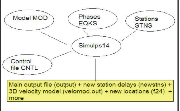
SIMULPS14 output files (Fig. 4.1) include the final 3-D tomography velocity field (from velomod.out file), the hypocenter parameters in hypo71 format (from file 13), the station corrections (from newstns file), the derivative weight matrix (from output file) and some statistics (from output and itersum files). Optionals are additional output files, such as the resolution matrix, the matrix having a-posteriori variance. In the main output file it is possible to check: the reduction of data variance per iteration, the hypocenter parameter adjustments, the rms per iteration, the model variance per layer and per iteration, the final resolution matrix diagonal elements, the a-posteriori variance per velocity perturbation and also the final and intermediate quake locations.

This inversion process is iterative and solves the problem by a 3-D tracer. The ray tracing approaches the wave path with the algorithms approximate ray tracing (ART) and pseudo-bending (Um et Thurber, 1987).

The program offers the interesting opportunity to compute synthetic travel times into the fort.24 file (see paragraph resolution assessment with synthetic tests). Synthetic travel times are computed for any synthetic 3-D structure with a set of quakes as illuminating sources. In this case, the quakes must be declared as shots and it is necessary to set the itmax control parameter (see file CNTL of all control parameters in the paragraph 4.3). Noise can be added to the synthetic travel times before relocalizing the events (the same that were used to

illuminate the synthetic structure). The relocalized events with their synthetic travel times are, then, inverted by using SIMULPS14 in a regular mode.

It is possible to check how the synthetic structure is retrieved by the 3-D inversion. The aim of inversion is to learn better about the resolution power of data-set and the geometry of the experimental set-up. This way, we can check how well the geometry and the amplitude of the synthetic structure has been retrieved and, furthermore we can examine what kind of artefacts are introduced into the final 3-D images.

As displayed in figure 4.1, at least four input files are necessary for SIMULPS14. They are:

◊ File CNTL (unit 01): control file. All switches that control the inversion are set in this file. ◊ File STNS (unit 02): station data file. This file includes the list of stations and a-priori station delays for both Vp and Vp/Vs . For each station, a flag is attached (0 or 1) in order to fix each correction individually (not working). In addition, this file includes the origin point and the rotation of the coordinate system (Km), which the user may choose for the model. It is advisable to choose the origin point near the center of the seismic network. If no rotation is required, the X axis points west, the Y axis points north and the Z axis points down.

◊ File MOD (unit 03): 3-D Node-grid and initial model. The set-up of this file needs some attention. The file describes the 3-D node-grid, the fixed nodes and a-priori Vp and Vp/Vs 1-D model. The steps that drive to the writing of the file are described in the next paragraph. ◊ File EQKS (unit 04): travel time data for earthquakes. It is also possible to invert for shots

(into SHOTS file) and for blasts (into BLAST file).

Examples and comments on these input files, applied to the data of our work, are given into the paragraph 4.3.

The a-priori model may have either a 1-D structure or a 3-D structure. However, it seems that the introduction of a 1-D structure, as the start point for the 3-D inversion, gets better results with respect to a 3-D structure (Eberhart-Phillips, 1989). In our approach, the starting velocity model will be the 1-D minimum velocity model as derived from step 1 and step 2 (fig. 1.8). If both Tp and Tp-Ts are used, two a-priori 1-D models are needed: one for Vp and one for Vp/Vs . The volume of investigation must be divided into nodes and each node is associated to an a-priori velocity value (introduced into the input file MOD). At the end, the code SIMULPS14 supplies a final velocity value at each node. The volume of investigation must be large enough, so that it encloses all rays. It is also possible to fix some nodes, so that the a-priori velocity values are not modified through-out the iterative process. Besides, the program is capable of fixing some of the free nodes during the inversion process

in cases of under-sampling (according to a criterion set in the control file). In that case, the code itself lowers the number of parameters to be inverted.

Figure 4.1: Main input and output files for SIMULPS14

The program stops if:

1. F-tests fails. This test verifies that the reference model itself is the least squares solution for a model having fewer degrees of freedom and this is not the case of an arbitrarily selected starting point (Kissling et al., 1994);

2. solution norm falls below a cut-off value (as specified in the CNTL file); 3. the number of iterations exceeds the value given to the CNTL file; 4. weighted data rms fall below a cut-off value given to the CNTL file.

More information can be found in the “user’s guide” (Evans and Eberhart-Phillips, 1994).

For the earthquake selection of the 3-D inversion all SISMANTILLES I events used in 1-D were relocated. Since the result is very sensitive to even a small number of bad data and quality control is essential we refrain from adding new data. In total 155 events with 6,671 observations were inverted (Tab. 4.1).

Number of selected events P-obs S-obs Total observations

155 4,054 2,617 6,671

Table 4.1: Number of events and observations selected for the 3-D inversion.

For SIMULPS14, model parameterisation should be based on the average station spacing and earthquake distribution (Haslinger, 1998). A model parameterisation, presenting a coarse grid of 18 x 18 km for horizontal plane, was used to account for the earthquake and seismic station distribution (Fig. 4.2). For vertical plane, spacing was of 6 km to 36 km depth. Therefore the grid dimensions for this inversion is characterized by 8 x 16 x 7 nodes. The boundary grid nodes of the model are not included; they serve only as numerical purposes and are automatically kept fixed.

This quite large grid represents a good compromise to detect the principal P- and S-wave velocity anomalies and to avoid both the under-determination of the problem and the strong reduction of the resolution. Indeed, if the grid is made very fine, x rays will not sample every node and the problem will be under-determined but, on the other hand, very small features can be detected with a very good resolution. On the contrary, if the grid is very large, each node area will contain several x rays, but, because the areas are now larger, small features cannot be detected by using a poor resolution (Menke, 1989). The over-determination factor of this inverse problem is roughly 2.8. In the following table we can see the number of knows and unknows parameters.

Knows Knows Knows Unknowns Unknowns Unknowns Overdetermination factor P-obs S-obs total model hypocentral total

4,054 2,617 6,671 1,792 620 2,412 2.76

Figure 4.2: Sketch of P-wave ray paths of 155

well-located seismic events traced before the computation of the 3-D model. Circles and triangles indicate earthquakes and seismic stations respectively.

Figure 4.3: Grid layout (red circles) in the plane for the 3-D inversion. Grid nodes are 18 km in longitude and latitude. Each epicenter is shown by a circle and depth. Land seismic stations and OBS are represented by blue triangles.

From the distribution of epicentres and stations (figure 4.2), it is clear that some grid nodes (figure 4.3) will never be hit by a ray. These nodes are fixed a-priori to reduce the number of unknowns. In the same way all nodes having a derivative sum (DWS, see paragraph resolution assessment) lower than 50 are kept fixed during the inversion.

The P-wave ray tracing (figure 4.2) gives us an idea of the resolution problem. If earthquakes occur within in a few kilometers from the surface, the rays are sub-horizontal and they sample only the zones under the stations, in this case we don’t find a good resolution of nearby surface structure. On the contrary, if the depth is of 15 kilometers we have a good sampling, for example the region corresponding to Martinique and Guadeloupe islands at this depth has a good resolution. If the depth increases up to 30 kms the resolution if better because we find an higher number of rays.

For the 3-D inversion, crustal velocities of the minimum 1-D model are extrapolated on the 3-D grid (Figure 4.3). On the figure 4.4 we can see this extrapolation for Minimum 1-D model derived from the a-priori Model 1 (Vp/Vs =1.76). The velocity of this new model has been linearly interpolated between the depth layering of the Minimum 1-D model. The Vp damping is a critical parameter in LET and his choice is one of the critical tasks to ensure meaningful inversion results (Eberhart-Phillps, 1986). Low damping values will lead to a complex model presenting a relatively large reduction in data variance, whereas high damping values will give a fairly smooth model having a small data-variance reduction.

Figure 4.4: Vp Minimum 1-D model derived from Model 1 (dashed line) and the corresponding initial reference model (solid line) for the 3-D inversion.

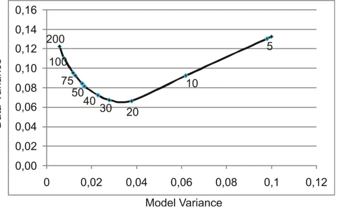
Resolution estimates, like the diagonal element of the resolution matrix (RDE, see paragraph resolution assessment), are also strongly dependent on the chosen damping values (Eberhart-Phillps, 1986), a damping value of 20 was chosen for the 3-D inversion. Indeed, by plotting data variance against model variance, the best damping value will be the one that greatly reduces the data variance without strongly increasing the model variance (figure 4.5).

Figure 4.5: Trade-off curve to determine the damping value for Vp inversion. A series of single iteration inversions has been performed with varying damping values. The chosen damping value of 20 compromises a significant decrease in data variance and a moderate increase in model variance.

The inversion is not done only for P-wave velocities but also for the Vp/Vs ratio. Due to fewer S-data and larger uncertainty in S-arrival time picks we presume larger not well resolved areas respect to the Vp tomographic images. We observe that, in these not well resolved areas, the initial Vp/Vs value will retain.

The program SIMULPS14 is applied to the our SISMANTILLES data-set. For the 3-D inversion, the mentioned input files (CNTL, STNS, MOD and EQKS) are required. An example of each file is presented below.

File CNTL

In this control file, the most important switches are: nitloc (the maximum number of iterations for hypocenter location), rmscut (the value for rms residual below which hypocentral adjustments are terminated), nhitct (the minimum DWS for a parameter to be included in the inversion), dvpmx (the maximum P-wave velocity adjustment allowed per iteration), vdamp (the damping parameter used in velocity inversion), i3-D (the flag for using pseudo-bending), nitmax (the maximum number of iterations of the velocity inversion-hypocenter relocation; for locations, just nitmax = 0 must be set, while to create synthetic data we must set nitmax = -1 and output synthetic data will be written into the file 24), iusep (in order to use P arrivals or not), iuses (in order to use S arrivals or not).

155 000 000 0.00 5 0 0 neqs,nshot,nblast,wtsht,kout,kout2,kout3 04 0.8 .020 0.1 -2. 25. 0.10 0.02 nitloc,wtsp,eigtol,rmscut(hyp),zmin,dxmax,rderr,ercof 05 1.5 0.5 0. 20. 20. 99.00 1.0 nhitct,dvpmx,dvpvsmx,idmp,vpdamp,vpvsdamp,stadamp,stepl 3 3 3 0.03 1 0.01 1 ires,i3-D,nitmax,snrmct,ihomo,rmstop,ifixl 500.00 900.00 2.00 3.00 5.00 delt1,delt2,res1,res2,res3 9 2 0.50 2.00 ndip,iskip,scale1,scale2 1.4 0.009 5 12 xfax,tlim,nitpb(1),nitpb(2) 1 1 0 iuseP,iuseS,invdelay 0 0 0 iuseq,dqmax,qdamp Table 4.3: Content of CNTL file.

We modified the default version of CNTL in order to consider the results of the inversion essays and the a-priori informations inferred from previous geophysical and geological studies.

 Vdamp is set equal to 20, according to the results of a series of inversions performed

 We set nitloc and nitmax equal to 3 because locations and velocities do not vary significantly in subsequent iterations

 We set i3-D equal to 1, as we use pseudo-bending

 We set nhitct equal to 10, as we choose a large grid spacing  We iusep = 1 and iuses = 1, as we invert P- and S- phases

File STNS

This file requires the origin of the coordinate system, and eventually its angle of rotation, as well as station coordinates and station corrections.

In our example, the BARB station, which is located in the Guadeloupe island, represents the center of the coordinate system. A rotation of 22° to the coordinate system is applied. We do not choose to introduce a-priori station corrections.

Table 4.4: content of STNS file.

File MOD

Now, in form of a recipe that follows three steps, we are going to describe how the file MOD can be build in our application.

The first thing to do is divide the volume investigation into nodes: the volume is divided into layers and each layer is divided into a 2D node-grid. The first layer must be chosen above the highest station. In our case, the LKGZ station is the highest one (1380 m), so we choose the first layer at 2000 m. On the other hand, a buffer zone must be introduced below the bottom of the volume and no event should belong to this zone. We choose the depth of the lowest layer at 750 Km below sea level. The ray geometry is indeed very peculiar. The ray cross sampling takes place into a small volume of investigation and we only invert for nodes that belong to this volume of investigation. However, we also have consider those events that are located outside the volume of investigation and enrich its ray sampling. Therefore, we suppose the bottom layer is 750 Km below sea level (hereafter bsl). The buffer zone is between 750 Km bsl and 36 Km bsl and no events belong to it. The nodes that belong to the top and to the bottom of the model are implicitly fixed. No need is required to specify their positions into file MOD in order to fix them.

15. 46.09 61. 10.21 22.00 0 106 SLBZ13N49.55 61W02.45 600 0.00 0.00 1 MCAZ13N51.02 61W01.14 615 0.00 0.00 1 to be continued ... MV3 14N33.28 60W53.35 0 0.00 0.00 1 LEY 14N50.81 61W06.74 0 0.00 0.00 1 FAJ 16N21.00 61W35.00 0 0.00 0.00 1 BARB16N13.93 61W29.65 0 0.00 0.00 1

Regarding the S-wave velocity model we suppose as constant relation Vp/Vs equal to 1.76.

The 2D grid-node (Fig. 4.3) must include the area inside the station network, plus a lateral buffer zone. Also some events should belong to the buffer zone and can be taken into account by SIMULPS14. The X-Axis points west and Y-Axis points north so, as a consequence, Z-Axis will point down. This means that the nodes belonging to the layers above sea level have negative z coordinates.

In the second step, apart from the border line, the fixed nodes (DWS <50) will keep their a-priori values of Vp and Vp/Vs as defined in the minimum 1-D model. The point: (i=1, j=1) is located on the bottom right-hand corner of the 2-D grid.

1.0 13 25 11 MODELE ANTILLES 20.07.10 -350. -90. -75. -60. -45. -30. -18. 0. 18. 36. 54. 72. 350. -350. -176. -160. -144. -128. -112. -96. -80. -64. -48. -32. -16. 0. 16. 32. 48. 64. 80. 96. 112. 128. 144. 160. 176. 350. -2. 0. 10. 20. 30. 40. 50. 60. 90. 150. 350. 2 2 2 3 2 2 to be continued ….. 0 0 0 4.60 4.60 4.60 4.60 4.60 4.60 4.60 4.60 4.60 4.60 4.60 4.60 4.60 4.60 4.60 4.60 4.60 4.60 4.60 4.60 4.60 4.60 4.60 4.60 4.60 4.60 to be continued…….. 1.76 1.76 1.76 1.76 1.76 1.76 1.76 1.76 1.76 1.76 1.76 1.76 1.76 1.76 1.76 1.76 1.76 1.76 1.76 1.76 1.76 1.76 1.76 1.76 1.76 1.76 to be continued……..

Table 4.5: content of MOD file

File EQKS

Regarding the content of the EQKS file, containing the phases of the local earthquakes, we can refer to sample given in table 4.6.

991127 9 8 33.79 16N40.75 61W54.13 94.61 3.00 196 34.0 0.17 0.1 0.1

BRGZ P 2 16.67CAGZ P 3 16.72CELC P 0 17.00DEGZ P 1 18.51-DEGZ SP3 14.95DOGZ P 1 17.03 ECGZ P 3 16.92FNGZ P 1 16.70LKGZ P 3 16.86LZGZ P 2 15.69MLGZ P 2 13.64PAGZ P 2 17.05 PAGZ SP3 13.96SEGZ P 2 15.50TAGZ P 3 17.04CELC SP1 14.21CHA P 0 18.05CHA SP1 15.22 LOU P 0 16.56LOU SP0 14.04

991129 1 8 27.39 14N49.12 60W49.94 100.00 3.00 283 11.0 0.45 -0.1 0.1

BAMZ P 3 14.77BIMZ P 1 16.13BIMZ SP2 12.83CPMZ P 1 15.43CRMZ P 2 12.06FDFZ P 2 14.90 FDFZ SP0 12.45GBMZ P 3 14.93LAMZ P 2 14.77LPMZ P 1 14.01MJMZ P 1 13.74MLMZ P 3 15.34 MLMZ SP2 12.05MVMZ P 1 13.96TRMZ P 1 15.35TRMZ SP2 12.31ZAMZ P 2 14.71ZAMZ SP2 12.07 to be continued……..

Table 4.6: content of the EQKS file.

4. 4 Local Earthquake Tomography of Lesser Antilles area

The 3-D inversion of the model with extrapolated velocities of the minimum 1-D model on the 3-D grid (figure 4.4) converged after 3 iterations, achieving a rms reduction of 37% and a data variance improvement of 60% referring to the initial 1-D model (table 4.7). We note that adjustments become insignificant after three iterations.

1-D → 3-D Rms Data variance

Start 0.38 s 0.15 s2

Final (3 iter.) 0.24 s 0.06 s2

Reduction to 1-D 37 % 60 %

Table 4.7: Data variance and rms reduction after 3-D inversion

Absolute P-wave velocity values are shown in figures 4.6 and 4.7, these tomographic results represent a somewhat averaged image of the crustal velocities. According to the resolution criteria and the synthetic tests (see paragraphs 4.5 and 4.6), the 3-D P-wave velocity structure is well resolved in the area delimited by the 250 DWS contour. Tomographic imaging reveals three distintict layers composing the island island arc crust. A lower crust (P-wave velocity 7.1 -7.3 Km/s) is underlain by a middle crust (P-wave velocity 6.8 -7.1 Km/s) and a thick upper crust (P-wave velocity < 6.8 -Km/s). The upper plate Moho is found at about 24 km below the sea floor.

4.5 Resolution assessment with the traditional tools

Assessing the resolution quality is of special importance in LET. A meaningful and reliable interpretation requires an accurate analysis of several resolution tools. Standard approaches comprise the use of hit count (HIT) and of derivative weight sum (DWS). These classical tools are available per default in the file named output of SIMULPS14.

Hit count is the simplest resolution estimate. It just counts the number of rays contributing to the solutions for a model parameter. Good resolution is associated with a high number of rays. The HIT does not account for the distance of a ray to a grid node, which is of great importance for the resolution. This restricts the use of HIT only for finding areas with no resolution. In SIMULPS14, the derivate weight sum value (DWS) adds up the geometrical

distance (weight) of each ray segment passing by a grid node to account for the distance of a ray to a model parameter.

Figure 4.6: Final solution of the 3-D inversion. We show the plane views of absolute wave velocity. 3-D P-wave velocity structure is well resolved in the area delimited by the DWS value of 250, see paragraph 4.5 for more details.

This way, DWS provides an average relative measure of the density of seismic rays near a given velocity node. This measure is superior to an unweighted count of the total number of rays influenced by a model parameter, since it is sensitive to the spatial separation of a ray from the nodal location.

Neither of the two measures, however, accounts for the directionality in the ray distribution that for resolution estimates is a crucial information. In fact, the solution for nodes that are sampled by rays showing mainly the same direction will strongly be coupled to the solution of adjacent nodes that are sampled by the same rays (Haslinger, 1998). Toomey et Foulger (1989) used the derivative weight sum of sampling of nodal location, which is defined as:

( )

å å ò

where i and j are the event and station indices, ω is the weight used in the linear interpolation and it depends on coordinate position, Pij is the ray path between i and j and N is a normalization factor that considers the volume influenced by αn. Thus, DWS gives some qualitative measurements of the total ray length in the vicinity of a model parameter and, therefore, good resolution is associated with a DWS value superior to a determined threshold. DWS values are shown in figures 4.6 and 4.7 by using respectively black and white contours, areas of reliable resolution are in general characterized by DWS larger than 250. This value of DWS threshold was derived on the base of tests, where we tried to recover a known velocity structure from a set of synthetic arrival times applying the inversion scheme under the same constraints as used for the real inversion problem (see paragraph 4.6). On the basis of these tests the 250 DWS threshold distinguishes better resolved zones from scarcely resolved ones where the significance of the patterns is questionable. The P-wave ray tracing (figure 4.2) gives us an idea about the resolution problem. If earthquakes occur within a few kilometers from the surface, the rays are sub-horizontal and they sample only the zones under the stations, therefore we cannot determine a good resolution of the areas near the surface structure. On the contrary if the hypocentre depth is at least of 15 kilometers we have a good sampling and the region of the central grid has a good resolution. If the depth grows the resolution if better because each ray crosses an high number of other rays.

Figure 4.7: On the left: Depth-cross sections positions, land seismic stations and OBS are represented by blue triangles, grid nodes by red circles. On the right: depth-cross-sections trough the 3-D P-wave velocity model. The white contour denotes DWS value. Black circles represent hypocentre locations after 3-D inversion.

4.6 Resolution assessment of the SISMANTILLES I data-set with synthetic tests of check-board model

DWS is a first-order diagnostic tool for the assessment of the resolution, whose real meaning depends on the individual conditions. We therefore try to corroborate our considerations of illumination and resolution with synthetic models. Compared to the diagnostics based on DWS, whose understanding needs intuition, the numerical experiments give an immediate and straight forward idea of the inversion stability, possibly insignificant or artificial features and the sensitivity with respect to the choice of the start model. Here we have been using synthetic traveltimes calculated for a check-board model. These data were then inverted using the same start model, parametrization and control values as for the real data. This approach follows the idea to verify damping and model parameterization and to test the resolution capability of the data set.

A check-board test (Spakman et al., 1993) consists of a series of alternating high and low anomalies, overlaid on a background model. Synthetic travel times are then calculated for this model and inverted. By comparing the results of the inversion of synthetic travel times with those obtained with the real data, we can estimate the restoring capacity of the data-set, areas of low resolution will be indicated by not restoring the check-board model (figure 4.8).

Figure 4.8: Top on the left: check-board synthetic input model on which travel times are calculated. From 6 to 30 km depth: results of the 3-D inversion for this synthetic data set. % velocity changes are given referring to those of the minimum 1-D model which provides the background model.

The comparison of resolution estimates based on DWS value with a synthetic test reveals the difficulty to define areas of good resolution simply by using a threshold. The test was carried out under the same constraints as the real inversion, i.e. using a damping value of 20.

In all layers of this test we find partly the anomalies regardless whether we consider input data. Plotting the parameters DWS with the inverted test velocity model we may establish suitable threshold values which can be used to distinguish fair resolved areas from scarcely resolved. In all layers we can delineate a reasonable identification of fairly resolved areas using threshold values of 250 for DWS. In figures 4.6 and 4.7 P-wave velocities images derived from this LET study, contours related to 250 DWS value mark areas of reliable resolution.

4.7 3-D Vp/Vs Model

Two main reasons exist to add waves readings to the 3-D inversion: first of all, S-phases add important constraints on the hypocentre locations. Second, the Vp/Vs ratio allows a more complete characterization of the mechanical rock properties. Unfortunately the use of S-waves in the 3-D inversion is limited due to their poorer quality and number of observations. To include S-waves readings in seismic tomography, two approaches are available: direct inversion of Ts for Vs (Benz et al. 1996) or inversion of Ts-Tp for Vp/Vs (Thurber et al., 1993). Normally exist fewer S-wave readings than P-wave readings in a data set, which may result in low resolution for Vs in areas of good Vp resolution. Inverting for Vp/Vs then guarantees a better resolution. The initial Vp/Vs ratio of 1.76, determined via Wadati diagrams, have been chosen on the basis of a recent analysis of IPGP observatories data-base (Clément, 2001). The damping value of 20 for Vp/Vs was chosen by a trade-off curve as it was done for Vp in paragraph 4.2.

Starting the Vp/Vs inversion with a 3-D P-wave velocity model and a constant Vp/Vs ratio guarantees that in areas where there is a good S-wave data coverage, deviations from the initial Vp/Vs ratio can be resolved, whereas in other areas the Vp/Vs ratio will remain at the average value. Of course Vp/Vs results will only be meaningful in areas where also reliable resolution for Vp is observed, so the results of the previous section should be taken into account.

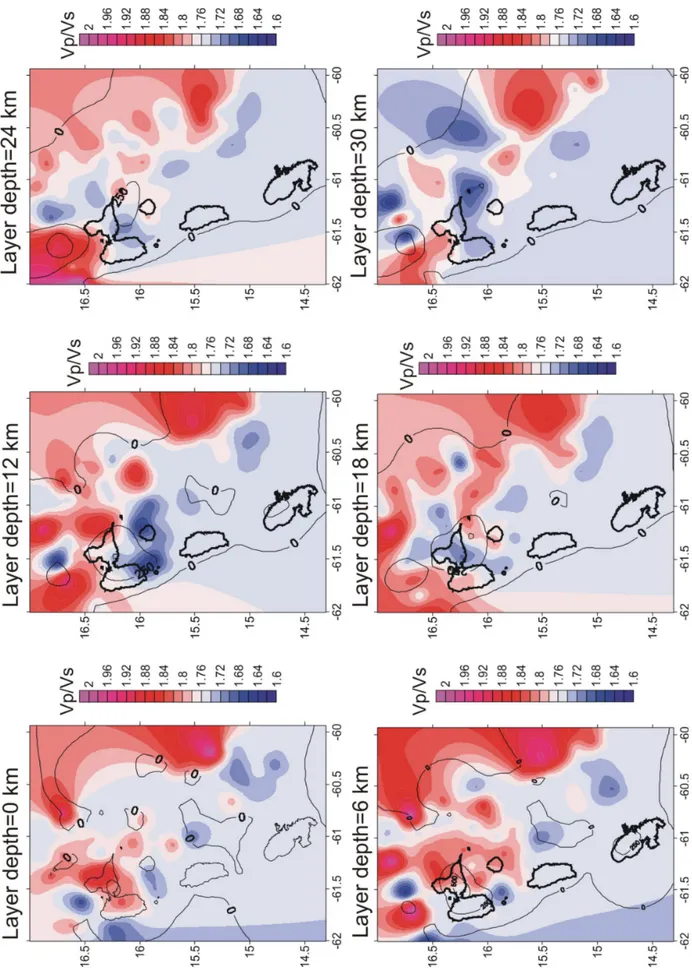
Figure 4.9: Results of the 3-D Vp/Vs inversion. We show plane views of absolute Vp/Vs ratio. Contours denote 0

Final Vp/Vs ratios that are shown in figure 4.9 are fairly well resolved only in small parts of the study area and offers, in general, no clear interpretation. Indeed due to the paucity of S-wave data (table 4.2) Vp/Vs ratio remains close to the starting value. The use of S-S-wave data therefore is linked to the first reason exposed in this section: S-phases add important constraints on the hypocentre locations.

In any case with regards the layer at 12 and kms depth striking is the low Vp/Vs ratio observed in southwestern of the Guadeloupe island, which coincides with the transition zone between the upper and middle island arc crust (see next chapter).