5. ANALYTICAL DEMONSTRATION 5.1. OVERVIEW

5. ANALYTICAL DEMONSTRATION

5.1. OVERVIEW

The purpose of this chapter is the calculation of the average duration of a step of a moving node. This parameter depends strongly on the simulation environment and it is unfeasible to calculate it for complex maps. However it is possible to study the case when the scenario is simple. The simplest case is when the simulation area is a rectangle with size [X, Y] without any obstacles and the pathway graph is composed by just one single destination vertex placed in the centre of the area. This simple scenario may represent the behaviour of a rectangular room inside a more complex scenario, from the moment a node arrives to the associated destination vertex till it leaves the room.

5.2. DURATION OF A STEP

We want to calculate the expectation of the random variable t:

( ) d E t E s   =    

where d is the distance between the initial and the final position of the node and s is the speed of the node.

Since d and s are independent,

( )

1 1 ( ) E t E d E d E s s     = _ ⋅ _= _{ }     (1)

The speed s is a random variable uniformly distributed between 1 and 5 m/s, so the variable z 1

s ≜ has a distribution:

( )

_{( )}

( )

( ) 2 1 1 1 1 4 5 S Z s g z f s f z z g s _{= −} z = = ≤ ≤ ′

Then the expectation is:

( )

( )

1 1 ln 5 4 E E z s  _{= =}     (2)

The distribution of the distance d changes depending on the status of the movement. When the node starts the movement from the destination vertex (or when it moves to it) just one of

the two points (initial or final position) has random coordinates. Instead, when the node is moving around the room in RWP movement, both of the two points are random.

Let’s assume that the node starts moving from the destination vertex. It moves for a random distance d, that has a distribution

( )

DV D

f d (where DV stands for “destination vertex”). Then the node will choose a random destination with probability rw (RWP model), or it will come back to the destination vertex with probability 1-rw (jumping into the graph). The probability of coming back to the destination vertex after k steps is:

(

) (

1

)

k

k

P =P X =k = −rw rw k=0,1,2,...

following a geometric distribution, which has a mean value:

( )

1 rw E X rw = −

So the node moves for k times for a distance with distribution

( )

R D

f d (where R stands for “random”) and 2 times (at the beginning and at the end) with distribution

( )

DV D

f d .

Then the expectation of d is:

( )

_{( )}

( )

( )

( )

( )

( )

1 2 2 2 2 2 2 R DV R DV E d E X E d E d E X rw rw E d E d rw rw = ⋅_ ⋅ + _ + − = + − − (3)

where ER( )d is the mean value of

( )

R D f d and EDV

( )

d is the mean value of

( )

DV D f d 5.2.1. Calculation of ER(d)

We want to calculate the distribution of the distance d, defined as:

(

) (

2

)

2

i f i f

d ≜ x −x + y −y

The coordinates of initial and final position have an uniform distribution in

[

0, X

]

for the x-axis and

[ ]

0,Y the y-axis. If ax is the difference between the two points along the x-axis,

x i f

a ≜x −x

It’s distribution is (Fig. 5.1):

( )

( )

( )

2 2 1 1 0 1 1 0 x x x A x X X x x a X a X X f a f x f x a a X X X  _{+ − ≤ <}   = ⊗ − =  _{− ≤ ≤}  Fig. 5.1 – Normalized fAx(ax)

( )

_{( )}

( )

( ) 1 2 2 2 1 1 1 2 2 1 1 0 x x x x x x A x B x x x x x x a b a g b f a f b a g a X X a b X X X b − ₌ =   = _′ =  −    = − ≤ ≤ Fig. 5.2 – Normalized fBx(bx)

Similarly, along the y-axis, by has a distribution:

( )

2 2 1 1 0 y B y y y f b b Y Y Y b = − ≤ ≤

The square of the distance between initial and final position is:

(

) (

2

)

2 _{2 2}

x i f i f x y x y

c ≜ x −x + y −y =a +a = +b b

So, the distribution is:

( )

( )

( )

2 2 2 2 2 2 1 1 ₂ 1 1 ₂ x y C B x B y f c f b f b X b rect X X X b b Y c b rect Y Y Y c b

δ

∞ −∞ = ⊗     − _{ }    −        _ _   _{ }  =      _{− −}        −      ₋       _{ }    

∫

i

The integral can be solved dividing it in three sections (assuming X ≤Y):

( )

2 2 2 2 2 2 0 2 2 2 2 0 2 2 2 2 2 1 1 1 1 0 1 1 1 1 1 1 1 1 c X C X c Y b c X X Y X b Y c b f c b X c Y X Y X b Y c b b Y c X Y X Y X b Y c b

δ

δ

δ

−     − − ≤ <     −          =  −  −  ≤ < −          _{ −  −  ≤ ≤ +}  _{  − } 

∫

∫

∫

The integral is:

2 2 2 2 2 2 2 2 2 2 1 1 1 1 1 1 1 1 2 2 2 arcsin b X Y X b Y c b b b b b X Y XY b c b X Y c b XY b b c b b b XY c X Y XY X Y δ δ δ δ δ    − − =    −    = − − + − −   ₋ = _ _+ − +  

∫

∫

∫

∫

∫

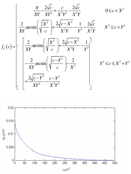
Calculating the integral for the three sections the result is (Fig. 5.3):

( )

2 2 2 2 2 2 2 2 2 2 2 2 2 2 2 2 2 2 2 2 2 2 2 2 2 2 2 2 0 2 2 1 2 arcsin 2 2 1 arcsin 2 2 arcsin 2 C c c c c X XY XY X Y X Y c X X c X c Y XY c X Y Y X Y c X X f c XY c X Y Y c Y Y c X Y XY c X c Y c Y XY X Y π  − + − ≤ <    _{ } −  _{ + − − ≤ <}           ₋     _{+ −}  = _{ }  _{ }   _{ }  _{   } − −  − ≤ ≤ +  _{ }        − −   + −           

C is the square of the distance. The distance d ≜ c has a distribution (Fig. 5.4):

( )

_{( )}

( )

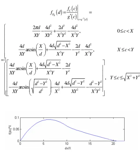
( ) 1 2 3 2 2 2 2 2 2 2 2 2 2 2 2 2 2 2 2 2 2 2 2 2 2 2 2 2 2 2 4 2 4 0 4 4 2 4 arcsin 4 4 2 arcsin 4 4 4 arcsin , , , R C D c g d f c f d g c d d d d c X XY XY X Y X Y d d X d X d d X c Y XY d X Y Y X Y d d X d X d XY d X Y Y d d Y d Y d Y d d XY d X XY X Y π − = = = ′ − + − ≤ < − + − − ≤ < = − + − − − − − − + −        _{ }   _{ }       _{ }   _{ }          2 2 Y c≤ ≤ X +Y             

Fig. 5.4 – fDR(d) calculated with XM=10 and YM=20

( )

R

( )

R D E d d f d

δ

d ∞ −∞ ⋅

∫

≜

it is possible to calculate the contributes of the three sections and then sum them together.

Section 1: 2 3 2 2 2 2 2 0 2 3 2 2 4 2 4 2 3 1 3 5 M X d d d d d d XY XY X Y X Y X X Y Y

π

_δ

π

  − + − =       = −  −  

∫

Section 2:

(

)

( )

2 2 2 2 2 2 2 2 _{2 2} 2 2 3 3 2 2 2 2 2 2 4 4 2 4 arcsin 2 2 1 4 3 3 arcsin 3 1 1 ln ln 2 2 2 2 1 3 3 6 Y X d d X d X d d d d XY d X Y Y X Y Y atgh Y X X _{Y X} X Y Y Y Y X X X Y Y Y Y X Y X X

δ

π

 _{  −}   _{ }+ − −  =            _{− +}  ₋    ₊  _{ − }    _{ }   _{ } + − +       − + − + −  +   

∫

Section 3: 2 2 2 2 2 2 2 2 2 2 2 2 2 2 2 2 2 4 4 2 arcsin 4 4 4 arcsin X Y Y d d X d X d XY d X Y Y d d d d Y d Y d Y d d XY d X XY X Y

δ

+  _{  −}   _{ + −}      =    ₋  _{− −} _{−  − + −}   _{ }     

∫

(

)

( )

(

)

(

)

2 2 2 2 2 2 2 2 _{2 2} 2 2 2 2 2 3 2 2 2 2 2 2 2 2 3 2 4 2 2 arcsin ln ln 3 3 3 2 2 1 ln 3 3 2 1 ln 2 13 1 3 1 16 30 15 10 6 15 2 1 3 2 Y X X Y X Y X Y X Y Y atgh atgh X Y Y X Y _{Y X} Y Y Y X X Y Y Y X Y Y X Y X X X X Y Y     = −  + + + −        ₊       ₋  _{− + +}       _{   − }  + _{ } _{+ + −}          + + _ − − _− − _ + _+     + + −

(

2 2

)

1

( )

ln ln 2 X Y X Y   + + +    

For the solving of the integral equations of Section 2 and 3, see Appendix B.

Summing the results of the three sections, the expectation of d is:

( )

( )

(

)

(

)

( )

(

)

( )

2 2 2 2 2 3 2 2 2 2 3 2 2 2 2 2 2 2 2 2 1 2 1 ln ln 2 3 2 1 1 1 ln ln 15 2 2 2 2 1 ln ln 3 3 15 13 1 3 30 15 10 R X Y X E d X atgh X Y Y Y Y X X Y X Y Y Y Y X Y X Y X X X Y X Y Y X   ₊       = + _{ }− + +  _{ }      + _ − + + + _     + _ + + − _+     + +  − −   

If X =Y the result becomes:

( )

2 2 1

(

)

ln 2 1 0.5214 15 3 R E d = X + − −  X  ≃ (4)

The same result has been already calculated in [13] in a different manner.

5.2.2. Calculation of EDV(d)

When the initial (or the final) position of the node is the destination vertex, positioned at ,

2 2 X Y

 

 

 , just one of the two positions is a random variable. So, assuming that the final

2 x i

X a ≜ x − The distribution is:

( )

1 2 x x A x X a X f a f x rect X X     =  − =      

For calculating EDV(d) the process is the same of the one used for ER(d). The variable bx ≜ax2 has a distribution:

( )

_{( )}

( )

( ) 1 2 1 0 4 x x x x A x B x x x _{a g b} x f a _X f b b g a ₌ − X b = = ≤ ≤ ′ Then 2 2 2 2 2 2 M M x i i x y x y X Y c _x − _ +_y − _ =a +a = +b b     ≜ has a distribution:

( )

( )

( )

2 2 2 2 2 2 2 2 2 2 2 2 2 1 ₈ 1 ₈ 4 4 0 4 2 arcsin 4 4 4 2 2 ₄ arcsin arcsin 4 4 4 x y C B x B y f c f b f b X Y b c b rect rect b X Y X b Y c b X c XY X X Y c XY c Y c X Y X Y c XY c XY c δ π ∞ −∞ = ⊗     − − −         = _{ }  _{ }   −   _ _  _ _      ≤ <      ≤ <    _{ }   =   −     ₊   − ≤ ≤     _{ }   _{ }  

∫

      

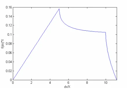
The distribution of the distance d ≜ c is (Fig. 5.5):

( )

_{( )}

( )

( ) 1 2 2 2 2 2 2 0 2 4 arcsin 2 2 2 4 4 ₄ arcsin arcsin 2 2 2 DV C D c g d f c f d g c d X c XY d X X Y c XY d Y d _{X Y} d X d Y c XY d XY d π − = = _′  ≤ <      _{≤ <}    _{ }  =    −    _{  +}   − ≤ ≤            _{ } 

Fig. 5.5 – fDDV(d) calculated with XM=10 and YM=20

Finally, the expectation of the distance is:

( )

2 2 2 2 2 2 2 2 1 1 6 12 1 ln ln 12 2 2 DV X Y X E d X Y atgh Y Y X Y X Y Y X  ₊    = + + _{ }     _{+ +}  _{ }     + _{ }−    _{ }    

( )

2 1

(

)

1

(

)

ln 2 1 ln 2 1 0.3826 6 8 24 DV E d =X + + − −  X  ≃ (5) 5.2.3. Final Results

So, if the area of the simulation is a square

[

X X,

]

and the destination vertex is positioned at ,

2 2

X X

 

 

 , we can calculate the average length of a step. Using the (4) and (5), the (3) becomes:

( )

2 2 0.5214 0.3826 2 2 0.7652 0.2438 2 rw rw E d X X rw rw rw X rw − + − − −   = _{ } −   ≃ (6)

and, using the (6) and the (2) in the (1), the average duration of one step is then:

( )

1 0.7652 0.2438 ln 5

( )

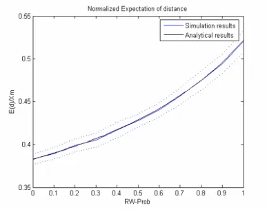
( ) 2 4 rw E t E d E X s rw −     =   _{ − }  ≃  

Figure 5.6 and 5.7 show the comparison between analytical and simulation results in the calculation of E(d) and E(t).

Figure 5.6 – Normalized E(d)