RFID-based smart shelving storage systems

Engineering PhD School “Leonardo da Vinci”

PhD Course in

“Applied Electromagnetism in Electrical and Biomedical Engineering,

Electronics, Smart Sensors, Nano-Technologies”

PhD Thesis

RFID-based smart shelving storage systems

ING/INF-02

Tutors:

Prof. Ing. Paolo NEPA ____________________________

Prof. Ing. Giuliano MANARA _______________________

Dot. Ing. Alice BUFFI _______________________

Author

Ing. Andrea D’Alessandro

________________

2014

2 Copyrigth © Andrea D’Alessandro 2014

3

CONTEST

Contest... 3 Journal Publications ... 5 Conference Publications ... 5 Introduction ... 7

1 Smart shelf overview ... 10

1.1 Introduction ... 10

1.1.1 Type of tags ... 12

1.1.2 Reader ... 14

1.1.3 Working Bandwidth ... 16

1.1.4 Physical Operating Principles ... 18

1.2 RFID Smart Shelf System ... 21

1.2.1 Localization in UHF-RFID smart shelves ... 25

2 A Localization Technique for Tagged Items in UHF-RFID Smart Drawers ... 33

2.1 Preliminary Analysis with a Static Drawer... 34

2.2 Classification Algorithms ... 40

2.3 Classification algorithm explanation ... 42

2.3.1 Geometric Interpretation ... 44

2.3.2 Static Result ... 46

4

2.4.1 Alghorithms K-means ... 48

2.4.2 Static Result K-Means ... 49

2.5 System Performance when Exploiting Drawer Sliding Actions ... 51

2.5.1 Choose of features number ... 57

2.5.2 Choose of features number ... 59

3 Smart Bookshelf ... 61

3.1 Introduction ... 61

3.2 Measures RSSI varying the phase of the fed antenna ... 65

3.2.1 Simulation ... 65

3.2.2 RSSI Measurement varying the fed phase ... 68

3.2.3 RSSI Measurement varying the phase and amplitude of the fed ... 72

3.3 Clustering Algorithm ... 74

3.3.1 Selection of the number of regions ... 75

4 Classification on Smart Shelf... 79

4.1 Input parameter ... 79

4.2 Classification in three zones ... 80

4.2.1 Labelling of the Regions ... 80

4.2.2 Classificator Performance ... 82

4.3 Classification in five zones ... 85

4.4 Result with different tag ... 87

Conclusions ... 91

5

JOURNAL PUBLICATIONS

1. R. Caso, A. D'Alessandro A. A. Serra, P. Nepa, G. Manara, “An Integrated Dual-Band PIFA for DVB-T and WiMAX Applications”, IEEE Antennas and Wireless Propagation Letters, publication year 2011.

2. R. Caso, A. D'Alessandro, A. A. Serra, P. Nepa, G. Manara, “A Compact Dual-Band PIFA for DVB-T and WLAN Applications”, IEEE Transaction Antenna Propagation on Communication, publication year 2012.

3. R. Caso, A. D'Alessandro, A. Michel, P. Nepa, G. Manara, “Integration of Slot Antenna in Commercial Photovoltaic Panels for Stand-Alone Communication Systems”, IEEE Transaction on Antenna Propagation, publication year 2013. 4. A. D’Alessandro, R. Caso, P. Nepa, “Dual band Integrated Antennas for

DVB-T diversity receivers”, International Journal of Antennas and Propagation, Received 6 December 2012; Accepted 30 March 2013.

5. A. D’Alessandro, A. Buffi, P. Nepa “A Low-Cost Localization Technique for Tagged Items in UHF-RFID Smart Drawers”, - submitted on IEEE Transaction Electronics Industrial

6. A. D’Alessandro, A. Buffi, P. Nepa, “A Phase-based Technique to Improve Tags Readability in UHF-RFID Systems” – under review to submission on Antenna Wireless Propagation Letters

CONFERENCE PUBLICATIONS

7. R. Caso, A. D’Alessandro, A. A Serra, P. Nepa, G. Manara, “Dual-band integrated G-PIFA antenna for DVB-T and WLAN applications”, 2011 IEEE AP-S International Symposium, Spokane, Washington, USA, 3-8 July 2011. 8. R. Caso, A. D’Alessandro, A. A Serra, P. Nepa, G. Manara, ”Wideband

integrated H-PIFA antenna for DVB-T and WiMAX applications”, 2011 IEEE AP-S International Symposium, Spokane, Washington, USA, 3-8 July 2011.

6

9. A. D’Alessandro, A. Buffi, P. Nepa, G. Isola, ”A new localization method for UHF-RFID Smart Shelves”, 2012 XIX RiNEm (Riunione Nazionale Elettromagnetismo), Rome, Italy, September 10-14, 2012.

10. A. D’Alessandro, A. Buffi, P. Nepa, G. Isola, “RFID-Based Smart Shelving Storage System”, 2012 Asia-Pacific Microwave Conference, Kaohsiung, Taiwan, 4-7 December 2012.

11. A. D’Alessandro, A. Buffi, P. Nepa, G. Isola, “A Localization Technique for Smart Bookshelves based on UHF-RFID Systems”, 2013 IEEE AP-S International Symposium, Orlando, Florida , USA 7-13 July 2013

7

INTRODUCTION

In recent years, RFID systems that are widely applied for the identification of objects and people in radio frequency, are also going to be applied used for localization purposes. In indoor applications (apartments, shopping malls, airports), conventional solutions can use a number of signal parameters: instant of arrival ( Time of Arrival , Time Difference of Arrival, TOA, TDOA), angle information (Angle of Arrival, AOA), phase information (Phase Difference of Arrival , PDOA ) or the amplitude of the received signal (Received Signal Strength Indicator, RSSI). There are also some scenarios with small dimensions where the location can be extremely useful. For example, in a hospital, a better service could be offered through RFID technology, as it can add more control to prevent human errors. Indeed, RFID technology can be useful for correct patient drug supply, dose recording, accurate dispensing, anti-counterfeiting as well as replenishment ordering; besides, it simplifies the information transfer between doctors and nurses (e.g. allergic reactions or drug treatment). In retail industry, real-time inventory based on RFID allows to monitor actual customer demand for products, to prevent an out-of-stock situation by timely replenishing orders, to increase sales through additional services (e.g. fitting rooms with smart mirrors providing suggestions to the customer). In food and restaurant industry, RFID technology allows for a better food control, as for example avoiding expired products sale. In this framework, RFID-based smart shelves, smart freezers, and proximity point readers have been developed in libraries, hospitals and retail industries.

In Chapter I, a brief introduction on RFID systems will be presented, in particular describing the main components involved and the principle of operation. It will be

8

described what is proposed in literature about RFID smart shelf and localization algorithms, with particular attention to the methods exploiting the RSSI information.

In Chapter II, an exhaustive experimental study by using off-the-shelf reader, antennas and tags, will be presented with reference to a wooden drawer filled with drug boxes. The LDA algorithm (supervised classifier) will be compared with the K-Means clustering algorithm (unsupervised classifier), to validate the proposed method. The procedure to get several RSSI average samples during the drawer sliding actions is described, and classification performance is investigated. First of all, an RSSI analysis is described with reference to a static configuration of the drawer (not sliding). Then, two classification algorithms are compared by considering a different number of drawer sub-regions. In the second part, the algorithm exploiting the drawer sliding is described and system performance is illustrated to verify the classification capability in a two-region drawer.

In Chapter III, a localization technique for smart bookshelves based on UHF-RFID systems is presented. Two off-the-shelf reader antennas attached to the bookshelf columns, one in front of the other, are used as an alternative to large-area thin planar antennas integrated onto the shelf top. Two scenarios were considered: the first one with a shelf that is D = 97 cm long, and the second one with D = 150 cm. Exploiting RSSI data acquired by the two antennas, a clustering algorithm is implemented to classify tagged books within one of the regions the shelf has been subdivided into. Preliminary results of the system performance analysis have been compared with simulations to demonstrate that is possible to create an interference region in different sectors on the shelf, through a proper phase shift between the feed currents of the two antennas. The system requires a power divider, a switch, variable phase shifters and finally a fixed or variable power attenuator based on the size of the shelf.

In Chapter IV the algorithm implemented will be described and then the performance results (in terms of normalized confusion matrix) will be presented and discussed. Finally, a preliminary analysis has been presented considering different tags, even if it is still under developing.

9

First and foremost, I would like to express my gratitude to Professor Paolo Nepa, my supervisor during PhD course. Thank you for countless discussions, hints, and nudges over the past years and for review of my the thesis. I would also thank Alice Buffi, my colleague. She collaborated in the development of my research for almost the entire doctoral period and she was co-author in the writing of the paper published for Conferences and Journals. For the material provided I would like to thank the CAEN RFID srl, in particular Gabriel Isola, for his useful explanations on RFID components and Andrea Iavazzo for support software. My sincere thanks to my colleague of the Microwave Laboratory, in particular Andrea Michel, remembering the beautiful past three years together.

Last but not least, I would like to thank my family and especially my wife, for all the support and encouragement to complete this experience.

10

Chapter I

1 SMART SHELF OVERVIEW

1.1 Introduction

The aim of Passive Radio Frequency Identification (RFID) is to identify objects, animals, people, through radio frequency (RF) transmissions[1]. The main advantage, respect at the well-known barcodes, is to detect object at more distance without direct visibility between transmitter and receiver (Fig. 1.1).

11

RFID technology consists of three basic components :

- Tag: is a transponder characterized by a small dimension, constituted by an

integrated circuit (chip) and connected to an antenna. It can be used into a container, embedded in a paper label, in a smart card, in a key, or integrated in electronic devices. The tag allows the transmission of data in short range without physical contact (Fig. 1.2).

Fig. 1.2 .An example RFID UHF tag

- Reader: The transceiver is controlled by a microprocessor and used to query

and receive information in response from the tag (Fig. 1.3).

Fig. 1.3. Typical reader UHF RFID

- Management System: is an information system which is connected with the

reader. This system allows users to get all available information associated with the objects and to maintain this information for the purposes of the application (Fig. 1.4).

12

1.1.1 Type of tags

There are three different kind of tags, everyone is characterized by a specific application based on energy management [2]:

- passive: referred to the fact that the mobile device does not have an

autonomous energy source like a battery, but is supplied via magnetic or electromagnetic fields by the base station. The signal transmitted by the reader is backscattered and modulated by the variation reflection coefficient of the antenna (Fig. 1.5a).

- semi-passive: equipped with a battery only used to feed the microchip, and not

to send a signal. In the transmission it has the same functionality of a passive tag (Fig. 1.5b).

- active: powered by a battery to transmit the signal: it is composed by

transmitter and receiver (Fig. 1.5c).

(a) (b) (c) Fig. 1.5 Example of UHF tags (Ultra High Frequency): passive, Lab-Id UH414 (a), semi-passive, CAEN

RFID A927Z (b), active IDN-ABG245AT (c).

Depending on the particular application it is necessary to adopt a type of tags rather than another: it is due to the special requirements in performance or in the forms (gain, directivity , sensitivity respect certain materials , use of the tag) [3]. The key is to get a good impedance matching the chip and the antenna of the tag. In this way it is possible

13

to optimize the tag performance (passive) because adaptation impedance depends on the amount of absorbed power .

The parameters which are used to compare the tags are: - sensitivity;

- read range of the tag;

- RCS (Radar Cross Section) differential tag ;

Passive tags sensitivity is the minimum level of power (or electromagnetic field) that is necessary to the activation. This parameter is independent from the characteristics of the reader and from the channel used for the transmission. Instead it depend on the threshold power of the chip (for example, the minimum power that is necessary to the activation the chip ), on the antenna gain and on a good matching between the antenna and the chip . These parameters can be expressed by the form (1):

tag th

P

= ⋅ ⋅ ⋅

G p

τ

P

(1) where G is the antenna gain of the tag, p is the polarization efficiency, τ is the impedance matching coefficient between the antenna of the tag and its chip, Pth is the

threshold power. This equation allows to know the minimum power that must be absorbed by the tag to make the chip in the condition to operate.

The read-range of the tag is the maximum distance at which the tag can be read. This feature not only depends on the sensitivity of the tag, but also from the EIRP (Effective Isotropic Radiated Power) of the reader and the channel on which is transmitted the signal. If you want to write on the tag, instead of reading, the range is not the same. In this case the range of the tag, called write range is the maximum distance at which the tag can be written. Usually the write range is smaller than read range, because in the writing operation it is necessary more power.

14

4

t t tag th

P G G p

r

P

τ

λ

π

⋅ ⋅ ⋅ ⋅

=

(2)

where Pt is the output power from the reader, Gt is the antenna gain of the reader. The

RCS (Radar Cross Section) differential comes from the theory of radar systems and characterizes the reflective properties of the tag with a complex quantity: it identifies the modulated signal power of "backscattering" by tag and received by the reader. It is a specific parameter of the tag and it depends on its characteristics and on the gain of the tag antenna and matching impedance between the tag antenna and the chip.

Fig. 1.6 The backscattering signal depend on the reflective properties of the tag with (RCS).

1.1.2 Reader

The reader is the element that, in RFID systems, allows to read the information contained in the tag [1]. In particular, the reader for passive tags (or semi-passive) must emit RF signals to provide tags with the energy required to response. It is worth noted the distinction between fixed reader (used in portals for accessing warehouses, conveyor, shelves) and portable reader. Typically to increase the read-range efficiency,

15

the reader transmit at the maximum EIRP, regulated by every country where the system has to work, using very antennas directives .

(a) (b)

Fig. 1.7 Example of common commercial reader: portable reader, R1240I-qID (a), and fixed reader R4300P-ION (b).

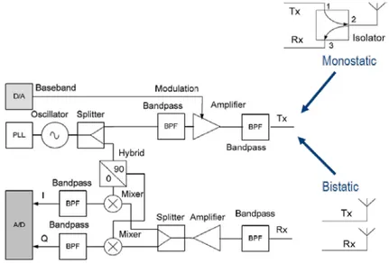
It is also important to obtain a good isolation between the channels of transmission and reception of the reader in order to detect and decode, in the best way, the weak signal from the tag [3]. The readers can be classified on these terms: transmission power, polarization and the gain or internal architecture . Basically, the reader can have two different structures : monostatic or bistatic .

16

The first one uses two different antennas for the transmitter and for the receiver. The second one uses a single antenna for the transmitter and the receiver, but needs an isolator that controls the signal path. It is worth noted that in the monostatic case the isolation parameter between the two channels , reception and transmission , is lower than the bistatic case. When the reader is limited in the size, the monostatic configuration is preferred [3].

1.1.3 Working Bandwidth

The frequency bands used in the communication between reader and tag depends both on the nature of the tag and on applications and are regulated by international and national organizations [1]. However, there are rules which changes, depending on the geographical areas and. this can often be incompatible when the object RFID tagged travels from a country to another. The band frequencies used in RFID technology are three:

- LF band, 120-145 kHz.

- HF band, centered at 13.56 MHz, considered the universal compatible band in

the world.

- UHF band the range 860 - 960 MHz can change in relation to the country. It is

a new RFID band chosen for logistic and objects tracking, due to a wider operation range than in LF and HF band .

- High UHF band centered at 2.4 GHz.

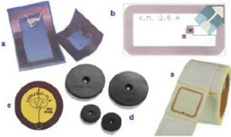
The choice of the working operation frequency affects on the read range of the system, interference with other radio systems, the speed of data transfer and the size of the antenna. The sub-band HF is the same regulated band in a lot of country, so it is the most popular band for RFID applications. The shapes of the tag available can be different. Typically, it is composed by an antenna formed with a coil of copper or

17

aluminum obtained by etching a thin metal layer thickness of a few tens of microns or by depositing on the same substrate with conductive inks,. The size and the number of coils determine the sensitivity and the operating distance, considering the power of the reader, too (Fig. 1.9).

Fig. 1.9 Different types of tags in the HF band: (a) tags on plastic support TI-RFID, (b) label LAB-ID (Italy), (c) and (d) tag for industrial use of EMS-group Datalogic (Italy), (e) X-ident label.

Today HF RFID systems and also LF RFID, have reached a good level of maturity. They are very popular because if used in the presence of fluid or tissue in the human body are not influenced. They are often used as smart labels (smart tags) used in the logistics and management of the objects. At this frequency also operate the contactless smart cards. These are widely used in the field of ticketing, to control access to particular services for which people have paid for, in the access control, or in the airport baggage tracking systems. A future development is expected in the field of banking transactions (ATM), credit cards , electronic passports.

Recently, it have been developed RFID systems in the UHF band. In this case the reader and the tags work in the far field (electromagnetic coupling) in order to obtain a series of the advantages respect to inductive coupling used at lower frequencies (LF and HF):

- transmission speed increased;

- smaller size of the antennas with the same performance;

- greater reader-tag communication distances (until 3 meters respect to 1.5 meters in the HF band);

18 - minor powers necessary for the chip to work,

- the beams of the antennas are closer resulting in restricted areas of reading. However, working in the UHF band, it is necessary to take into account the interaction with the material of the object on which is placed the tag and from the possible reflections of electromagnetic radiation caused by the presence of nearby objects. These factors increase the noise at the receiver input. The system is therefore more sensitive to the environment.

1.1.4 Physical Operating Principles

The space around the antenna can be divided into two regions, Near Field region (NF) and Far Field region (FF). In FF the electric and magnetic fields propagate through space as an electromagnetic wave; they are perpendicular to each other and to the direction of propagation. The electric and the magnetic field decrease as 1/r , where r is the distance from the antenna. In the NF field components have different angular distributions and decrease as 1/r ³. Moreover the near-field region can be divided in other two regions: Reactive Region, where the energy is not propagated but is stored and Radiating Region, in which the angular distribution of the fields depends on the distance and the antenna begins to radiate energy, as shown in Fig. 1.10, [1].

19

In passive RFID systems, the communication between reader and tag is due to electromagnetic coupling (in the far field UHF) or via inductive coupling (near field, in-band LF, HF).

Inductive coupling (magnetic) in near field conditions. In this case, where the

distance is smaller than the wavelength emitted by the antenna of the reader, the effect of the current induced by the magnetic field variable in the time periodically is prevailed on the tag [2], (Fig. 1.11).

Fig. 1.11 Inductive coupling in the near field (Systems LF / HF).

According to Lenz’s law, the tag is immersed in a magnetic field, the magnetic flux variable in time is concatenated with the coils of the antenna tag inducing a current in the coils itself. The inductive coupling between the reader antenna and the tag is then carried out as in a transformer. The energy obtained is used to activate the tag.

From the electrical point of view, the two antennas represent an L-C circuit (inductance - capacitor) where, at the resonant frequency, the energy transferred between reader and tag is maximized. The communication between transmitter and receiver is obtained modulating in amplitude the magnetic field generated by the reader antenna with the digital signal in base band that must be transmitted. The receiver circuit of the tag recognizes and decodes the modulated field , from this, the information is transmitted by the reader. Instead, the communication from the tag to the reader is occurred through inductive coupling, since a passive tag is not fed This occurs as in a

20

transformer where the secondary winding (tag antenna) varies its load, the result is seen from the primary winding (reader antenna) . The tag chip achieves this effect by changing the impedance of the antenna in accordance with a modulating signal, obtained by reading data in its memory.

Electromagnetic coupling conditions in the far field. In this case, where the

distance is greater than the wavelength emitted by the antenna of the reader, the effect of electromagnetic field variable in the time periodically is prevailed on the tag.

The antenna of the tag reflects to the antenna reader a part of the electromagnetic power received by the interrogation signal emitted by reader (Fig. 1.12). The reflection phenomenon of the electromagnetic waves is known as backscattering and is the same principle on which radar systems are based. The signal is modulated by varying the impedance of the antenna tag that changes its state from absorbent to reflective and vice versa. The condition of the far field is obtained for d >> λ , where d is the distance between transmitter and receiver and λ is the wavelength .

Fig. 1.12 Electromagnetic coupling in the far field (UHF systems).

In general, the field distribution of the RFID system can be influenced by the presence of certain objects. For systems that work with inductive coupling (typically used in the LF band and HF), most of the reactive energy is stored in the magnetic field and are particularly influenced by objects with high magnetic permeability (even if are not objects of common use). Therefore, these systems can work in close proximity to

21

liquids and metals without consequences. On the other hand, the systems exploiting the capacitive coupling, where the majority of the reactive energy is stored in the electric field, are influenced by the presence of objects with high dielectric permittivity and high loss [1].

1.2 RFID Smart Shelf System

UHF Radio Frequency IDentification (RFID) technology is gaining increasing attention for Item-Level-Tagging (ILT) applications [4]-[5]. In a hospital scenario, a better service can be offered through RFID technology, as it can add more control to prevent human errors [6]-[8]. Indeed, RFID technology can be useful for correct patient drug supply, dose recording, accurate dispensing, anti-counterfeiting as well as replenishment ordering; besides, it simplifies the information transfer between doctors and nurses (e.g. allergic reactions or drug treatment). In retail industry, real-time inventory based on RFID Smart Shelves [9] allows to monitor actual customer demand for products, to prevent an out-of-stock situation by timely replenishing orders, to increase sales through additional services (e.g. fitting rooms with smart mirrors providing automatic suggestions to the customer, Fig. 1.13).

22

In food and restaurant industry [9], RFID technology allows for a better food control, as for example avoiding expired products sale (Fig. 1.14). In this framework, RFID-based smart shelves, smart freezers, and proximity point readers have been developed in libraries, hospitals and retail industries[10]-[13].

Fig. 1.14 RFID applications in supermarket.

In addition to an automatic real-time inventory, item localization can be useful as well and the UHF-RFID passive technology represents a low-cost radio-localization technique for indoor scenarios [14]-[19]. Indeed it allows for developing additional capabilities, as for example to avoid misplaced items in pharmaceutical industry (e.g. missing sales due to drugs in wrong drawer, Fig. 1.15) or in retail industry [20] (e.g. items left on the wrong shelf by the customers, products forbidden or lost in the fitting room).

23

Some companies have proposed systems for the management of libraries, among them it is worth mentioning the Bibliotheca RFID Library Systems with the Biblio Chip RFID [21], and the LibBest with the RFID Library Management System [22] (Fig. 1.16).

Fig. 1.16 RFID Library Management System described in [22].

An interesting type of smart shelf system is that proposed by Capture Tech (a division of Barcoding Inc.) called Active Shelf System [23]. It is used for tracking and locating objects in scenarios such as shops, pharmacies, libraries or warehouses, or any kind of environment that involves the of objects on shelves or racks placement. In particular , a single reader is used to control a large number of antennas that radiate at different time instants, as illustrated in Fig. 1.17. They are arranged in the shelves in order to divide the area of inventory in resolution cells. Each antenna generates a distribution field confined in a restricted area of the shelf in such a way that the tag is identified by the single antenna that receives a greater power. It worth noted that to improve the accuracy, it is necessary to increase the number of antennas in spite of the a major complexity of the system. The database containing the inventory of tags that are always updated with the reading procedures at regular intervals, or it is possible use the motion sensors on the shelves to update the database as soon as a tagged object are added or removed.

24

Fig. 1.17 “Active Shelf System” proposed by CaptureTech [23].

Another interesting product distributed by Meps Real Time Inc., called Intelliguard, Automated Dispensing Cabinet [24], uses a UHF passive RFID management of medicines that can monitor the presence of drugs inside a chest of drawers. It is a simple inventory system that does not provide localization (Fig. 1.18).

25

1.2.1 Localization in UHF-RFID smart shelves

For localization purposes in passive UHF-RFID smart shelves, simple solutions propose to localize tags on the basis of their presence/absence within the read range of a reader. Thus tag localization is possible just in a specific area within the scenario and with a low/coarse grained resolution. This is the same principle exploited in HF systems and described in [25], where a multi-antenna arrangement is designed for smart drawer chest to distinguish among tagged items within four regions inside the drawer. Typically, to achieve this goal in UHF-RFID systems, ad hoc reader antennas radiate a spatially confined electromagnetic field [26]-[30]. Indeed by exploiting the near field (NF) coupling [31]-[33] between reader antennas and tags, only items close to the reader antenna are detected and cross readings of items placed on other shelves are avoided (see false positive issue discussed in [34]).

For more accurate localization in passive UHF-RFID smart shelves, both amplitude and phase [35] of tag backscattered signal can be exploited since the reader performs a fully coherent detection and at the best of the authors’ knowledge, only few authors have addressed the problem [36]-[38]. The amplitude information of the tag backscattered signal is already available at the output log-file of any commercial reader in terms of Received Signal Strength Indicator (RSSI), thus it is the most widely employed [36]-[37]. In [36], a KGNN (K-Size Grouping of Spatially Nearest Neighbor) algorithm is proposed with multiple reader antennas and reference tags. Different interrogation zones are selected on the basis of the reader antennas detecting the target tag (i.e. tag to be located); within the above regions, groups of K nearby reference tags are considered. On the basis of similar RSSI values and number of readings, one group of reference tags is chosen for each reading zone and finally they are employed to calculate the target tag coordinates (scenario shown in Fig. 1.19).

26

Fig. 1.19 Smart shelf with 6 boxes equipped with UHF tag 16 and reference tag, used in [36].

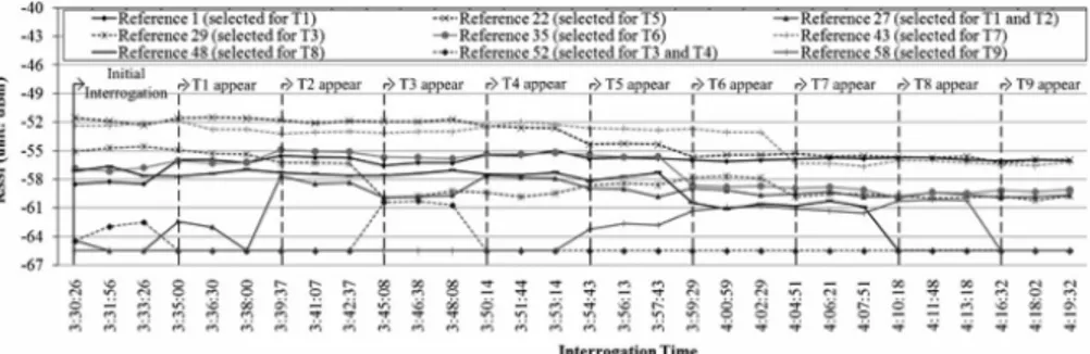
By using two commercial reader antennas (located outside the shelf) and 16 reference tags, a 23 cm estimation error is obtained for a shelf of 91 x 144 cm2 and six target tags. Instead in [37], the localization algorithm utilizes detected changes in the tag readability to infer the presence of neighboring tags (measurement set-up shown in Fig. 1.20).

27

Fig. 1.21 RSSI Measurement, during the new tags insertion (T1, ... T9) in the scenario

Indeed, a new tag added in the scenario can influence the RSSI of reference tags (tag-to-tag interference, Fig. 1.21); groups of reference tags experiencing higher RSSI variations and spatially close are chosen to calculate the target tag position. By employing one commercial reader antenna (located outside the shelf) in a 91 x 152 cm2 wooden shelf with 60 reference tags and nine tagged items, a mean estimation error of around 10 cm is achieved. It is expected that performance of such localization methods depends on number of reference tags; by using few of them, the accuracy can be notably reduced; on the contrary, a better localization accuracy can be achieved if using many reference tags, despite of less available readings for each target tag and higher computational cost. Obviously a bound exists after which by increasing the number of reference tags the computational cost increased without improving the localization accuracy [39]. It is noteworthy that, as alternative to reference tags and multiple readers deployment, the RSSI could be employed to determine an accurate empirical path loss model as in classical indoor scenario[40]-[41], but the Friis equation cannot be used to describe a power-distance model in scenario of the same order of the wavelength, as in smart shelves at the UHF band, and a more-complicated accurate path loss model should be derived.

As alternative to amplitude-based method, the phase of the tag backscattered signal can be employed. Such phase depends on both the propagation channel and the modulating properties of the tag that are frequency and power dependent. However, when the phase difference of arrival (PDOA) is applied, such factors can be easily

28

filtered out [35]. An example of a phase-based localization technique for smart shelves has been proposed in [38], in Fig. 1.22 is represented the scheme of realization.

Fig. 1.22 Shelves with antennas cascade as the reader antennas [38].

A cascaded reader antenna is integrated into the shelf and the tagged item location is estimated by processing the phase information of tag backscattered signals at two different frequencies. The antenna has been realized in coplanar line technology (Fig. 1.23) to work in the near field, in order to be able to read an object placed on the shelf avoiding to radiate above the shelf itself (about 12 cm).

29

The location of the tag on the shelf occurs by using the phase difference between the signal transmitted and received by the reader. This measure is proportional to the path that go through the re-irradiated signal from the tag and thus allows to locate it with an accurate estimate (with an average error of just over 4 cm). In particular, in the phase of initial calibration of the system, the path that performs the signal can be calculated knowing a priori the length of the both cables and the structures of antennas guiding (covering the whole space of the shelf as shown Fig. 1.24).

Fig. 1.24 Cascaded Antennas on Shelf

This antenna, typically working in UHF bands but with characteristics of a radiation pattern which is adapted to operate in near field. In this way the electromagnetic field remain confined in small volumes and well defined to avoid readings outside of this boundary and also leaving uncovered areas.

Typically it has dimensions that can easily be adapted for a shelf of a library and roller conveyor. to be positioned horizontally along each shelf of any materials (including metal). The antenna has been designed with a typical microstrip technology, closed on a matched load (Fig. 1.25) . The overall dimensions, obviously with structural limits, dependent on the wavelength , can be chosen ad-hoc in order to be able to cover the exact area of a shelf (a typical size may be 30x100 cm) .

30

Fig. 1.25 Smart shelf configuration: (a) straight line; (b) meandered line

The effect of field distortion on the edges of a microstrip is called Fringing Field is exploited to coverage the volume of a shelf. (Fig. 1.26).Moreover, in this case, it tends to use a substrate with low permittivity in order to increase this effect, considering also the thickness as the second parameter of the project (in addition to the substrate material).

Fig. 1.26 Fringing Field effect on microstrip antenna

In this way, the ground plane has two effects: the first is to isolate the part below the antenna, the second is to cover the whole platform, ensuring that the field is distributed throughout the area. Finally the electromagnetic field remains confined over the antenna above the shelf; it is due to the characteristic of not radiate in the direction orthogonal to the line itself (in this case upward).

In literature field distributions measurements are obtained and shown in Fig. 1.27. They are evidence of how the fields remain confined in the volume of a shelf in all directions of the plane x, y, z . In addition, the strong field is along z and y; this makes possible a good reception in different possible orientations of the tag, which is in near field region.

31

Fig. 1.27 Field distribution simulated: near field components (Ex, Ey, Ez) and near field total field (Et) at working frequency of 866MHz.

Subsequently to the insertion of books in the shelf, the fields experience an increase in amplitude due to the fact that the waves tend to concentrate in the vicinity of the books, and therefore to disperse in a significantly less in the surrounding environment, but remain confined in the desired volume, it shows the experimental results in Fig. 1.28 [27].

To validate the coverage efficiency, this antenna was applied to a shelf with some books tagged to verify how many of them can be read. Regardless orientation of the tag are obtained a Read Rate of 100% within the shelf along the x-axis, y or z while the readings fail (0%) exactly along the four extremes (black crosses), demonstrating the effectiveness of the containment of the reading volume.

32

It worth be noted that in applications with a large amount of tags, it could be helpful to determine the presence of tagged items in a specific region of the shelf, or if an RFID-tagged drug box is in a specific sector of a pharmacy drawer [25], rather than giving the spatial coordinates of the tagged item.

Indeed, in next chapter, it will be presented an exhaustive experimental study by using off-the-shelf reader, antennas and tags, with reference to a wooden drawer filled with drug boxes. The employed LDA algorithm (supervised classifier) will be compared with the K-Means clustering algorithm (unsupervised classifier), to validate the proposed method independently from the classification algorithm that is going to be used. The procedure to get several RSSI average samples during the drawer sliding actions is described, and classification performance is investigated

33

Chapter II

2 A

LOCALIZATION

TECHNIQUE FOR TAGGED

ITEMS IN UHF-RFID SMART DRAWERS

In this chapter will be presented a new localization method for UHF-RFID smart drawers. The main idea is to detect the presence of tagged items within a drawer region, by exploiting various RSSI measurements acquired during the drawer opening/closing actions. Indeed the relative position between reader antenna and tags changes during the drawer sliding, so allowing for several RSSI measurements. This is the innovative concept with respect to a conventional technique where RSSI data are collected when the drawer is closed and several antennas for each drawer are used to increase the number of RSSI samples per tag. Such RSSI data can be employed fruitfully in a classification procedure to identify the presence of tags in one of the predefined drawer regions and preliminary results have been presented employing a Linear Discriminant Analysis (LDA) algorithm. Only one reader antenna is needed for each drawer; also, no mechanical system for assisted sliding actions is necessary.

34

2.1 Preliminary Analysis with a Static Drawer

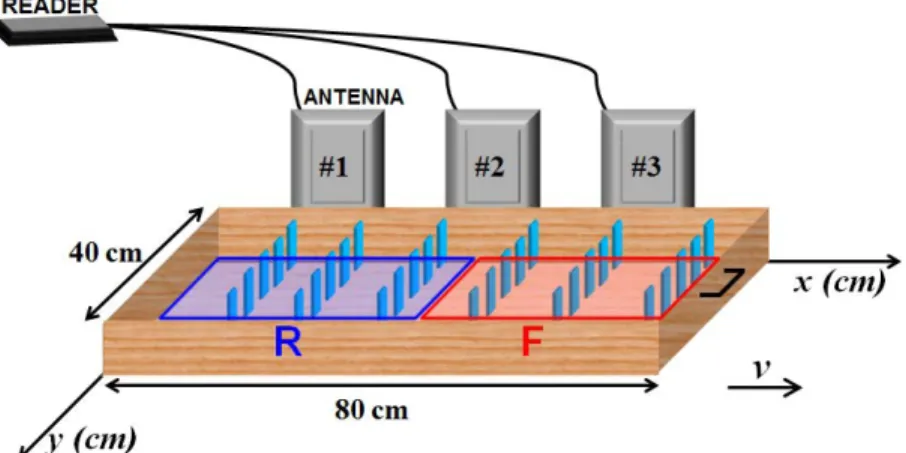
A preliminary study has been carried out by considering a drawer in a static configuration (not sliding), to investigate RSSI distribution inside the drawer and the potentials of a classification algorithm for tag localization. It is noteworthy that in this context tag localization stands for tag classification within one of a set of predefined regions of the drawer, and not for tag coordinates estimation. Indeed, the above objective could be useful in such scenarios where precise localization is almost useless, and it is difficult to settle on a path loss model to estimate the tag position from RSSI measurements (drawer size is of the same order of the free-space wavelength).

An 80 x 40 cm2 wooden drawer has been filled with 42 drug boxes of different size (Fig. 1.1). Each paper box has been tagged with an UPM Raflatac Rafsec G2 tag (Fig. 2.2a) [42]. Commercial reader and antenna are employed: the CAEN RFID R4300P ION reader (Fig. 2.2b) with the CAEN RFID WANTENNAX007 linearly polarized antenna (Fig. 2.2c) [43], (circularly polarized antennas should be used with arbitrarily oriented tagged boxes). A polarization matching condition between reader and tag antennas has been considered (vertical tags are in the reader antenna E-plane). The reader is able to detect up to 100 tag/s and the conducted output power has been set to 27 dBm.

35

(a)

(b)

(c)

Fig. 2.2 Equipment employed during the measurement campaign: (a) UPM Raflatac Rafsec G2 UHF tag, (b) CAEN RFID R4300P ION reader and (c) CAEN RFID WANTENNAX007 linearly polarized antenna

Preliminary measurements have been carried out with a static drawer configuration, by considering three reader antennas sequentially fed and placed at different positions with respect to the drawer, as sketched in Fig. 2.3, (they resemble three instantaneous reader antenna positions during drawer sliding). The drawer movement is parallel to the

36

x-direction and during sliding the reader antenna changes its position with respect to the drawer.

Fig. 2.3 Measurement setup for three reader antennas placed in various positions beside the drawer, along the x-direction

The drawer movement is parallel to the x-direction and during sliding the reader antenna changes its position with respect to the drawer. As shown in Fig. 2.4 the RSSI distribution is represented for the reader antenna near the corner (position #1 in Fig. 2.4a and position #3 Fig. 2.4c) and in the middle of the drawer (position #2 in Fig. 2.4b). For each tag an averaged RSSI is shown (the mean value has been calculated by averaging on 20 RSSI samples). The graphs represent a sampling distribution that is dependent from both the reader antenna location and the tag positions within the drawer (in this case tags are aligned in six columns). It is clear from Fig. 2.4 the problem already discussed in [36] of the RSSI ambiguity, since tags in various positions could respond with equal RSSI value. Furthermore, it is worth to noting that in such scenario (drawer size is of the same order of the free-space wavelength) it is difficult to settle on a path loss model to estimate the tag position from RSSI measurements.

37

Fig. 2.4 RSSI map of 42 tagged drug boxes uniformly distributed inside a 80 x 40 cm2 wood drawer and a linearly polarized reader antenna: (a) near the corner of the drawer (position #1 in Fig. 3) and (b) in the middle

38

The possibility to distinguish among M=2 drawer regions (rear region, R, and front region, F) has been investigated through a scatter plot analysis. Results are illustrated in Fig. 2.5- where each point corresponds to a set of RSSI samples (one sample for the fed antenna), for a given tagged box. Different markers indicate tags belonging to different regions; an equal number of tags has been considered for each region (R-region tags are represented with blue circle markers and F-region tags with red triangle markers). Actually, each RSSI sample has been obtained as a time average on 20 RSSI recorded samples, to filter out RSSI fluctuations due to the manufacturing process, thermal noise, and other environmental effects. By only exploiting the RSSI data at the antenna #1 (RSSI1) the point clouds are overlapped (Fig. 2.5a), so showing that in this case it is not

possible to distinguish among tags belonging to the two predefined regions (one RSSI value is not characteristic of a certain region).

Fig. 2.5 Scatter plot of measured RSSI values by using various reader antennas beside the drawer and 42 tags uniformly distributed in M=2 drawer regions: antenna #1

By employing two RSSI data for each tag (samples measured by sequentially fed antennas #1 and #3, named as RSSI1 and RSSI3) the point clouds become more separated

39

Fig. 2.6 Scatter plot of measured RSSI values by using various reader antennas beside the drawer and 42 tags uniformly distributed in M=2 drawer regions: antennas #1 and #3,

Furthermore, by employing three RSSI samples (those acquired by sequentially fed antennas #1, #2 and #3, named as RSSI1, RSSI2, RSSI3) the point clouds appear clearly

separated Fig. 2.7

(c)

Fig. 2.7 Scatter plot of measured RSSI values by using various reader antennas beside the drawer and 42 tags uniformly distributed in M=2 drawer regions: antennas #1, #2 and #3.

40

Above results suggest that several RSSI data acquired by a number of sequentially fed reader antennas beside the drawer (or equivalently for various positions of a single reader antenna during a drawer sliding operation) can be employed as features (input parameters) of a classification algorithm.

2.2 Classification Algorithms

On the basis of scatter plot analysis shown in previous section, the possibility to distinguish among tags in either M=2 drawer regions (R and F regions Fig. 3.1) or M=3 drawer regions (R, C and F regions in Fig. 3.1.b) is here investigated for the static drawer configuration by using {RSSI1, RSSI2, RSSI3} values acquired by sequentially

feeding all three reader antennas (Fig. 3.2), namely N=3 classification features have been considered. Two different classification algorithms have been applied and compared: a Linear Discriminant Analysis [44] and a K-Means algorithm [45].

Fig. 2.8 Drawer scenario with 36 tagged drug boxes (target tags) and 6 reference tags in the middle of the drawer: M=2 drawer regions

41

Fig. 2.9 Drawer scenario with 36 tagged drug boxes (target tags) and 6 reference tags in the middle of the drawer: M=3 drawer regions.

The LDA method is a supervised classification algorithm [44], where classes are known a priori (the latter are the drawer regions which tagged items belong to). For the training procedure, up to six reference tags have been considered within the drawer, two or three for each region (Fig. 3.1, Fig. 3.2 respectively) . Thus the classifier employs RSSI samples related to them to learn class characteristics. It is worth noting that this training process is done simultaneously with the classification process since both reference and target tags are detected during the same inventories. As a consequence a separate calibration procedure is not required. The LDA algorithm finds a linear transformation (i.e. discriminant function) of the input features that yields a new set of transformed values providing a more accurate discrimination than either features alone. A transformation function is chosen in such a way to maximize the ratio of among-class variance to within-class variance (e.g. dense point clouds that are well separated in a scatter plot representation). As for example, in a 3D problem, the transformation has the purpose to project the three features in a new 2D plane such that the distance among groups is maximized. Finally, the classification is done on the basis of a minimization of the distance from the group barycenter in the transformed space. Different distance criteria can be adopted and the Euclidean distance has been chosen in this study.

42

2.3 Classification algorithm explanation

The classification algorithm type DLA substantially provides the use of an estimator MAP (Maximum A Posteriori Probability) with Gaussian model that involves the construction of a linear discriminant function [46]. For each target tag there is a function that is built and based on its maximum value, it must decide whether it belongs to a class or another. The algorithm can therefore be described by the relation (3):

(

| )

(

| ),

i i j

x

∈

Z

se P Z x

>

P Z

x

∀ ≠

i

j

(3)

where x refers to the RSSI value of target tag (after average operation on RSSI acquired from the tag) and Zi the i-th area. In (1) it is affirmed that a target tag belongs

to an area where the posteriori probability is the maximum based on RSSI values acquired. This concept can also be expressed in another form, in fact, using Bayes' theorem, equation (1) can be rewritten as a function of the probability density (4)

( |

) ( )

( |

) (

),

i i i j j

x

∈

Z

se f x Z P Z

>

f x Z P Z

∀ ≠

i

j

(4)

where statistical terms can be derived from reference tag values (training data). By defining the discriminant function as (5):

( )

=

ln[ ( |

)] ln[ (

+

)]

i i i

g x

f x Z

P Z

(5)

the (2) can be expressed in abbreviated form as (6):

( )

( ),

i i j

43

In (6) it can be meant that the algorithm associates a target tag to that area for which the discriminant function assumes maximum value. In our case, the discriminant function is linear and it can be assumed as a Gaussian distribution model. Moreover the conditional probability density can be expressed in its form known in the literature (7):

1 2 1 2

1

1

( |

)

exp

(

)

(

)

(2 )

π

|

|

2

−





=

_

−

−

−

_





T i L i i i i

f x Z

x

m

C

x

m

C

(7)

in which the statistical parameters mi and Ci are: the vector of mean values and the

covariance matrix of the reference tag belonging to the i-th area respectively, in order to specify the features of that area. By imposing this hypothesis the discriminant function assumes the form (8):

1

1

1

( )

ln[ (

)]

ln |

|

(

)

(

)

2

2

T i i i i i i

g x

=

P Z

−

C

−

x m

−

C

−

x m

−

(8)

Summarizing, the decision rule becomes (9):

1 1 ln | | ( ) ( ) ln | | ( ) ( ) ln[ ( )] ln[ ( )] 2 2 − − ∈ + − − + − − − > − ∀ ≠ i T T j j j j i i i i i j x Z se C x m C x m C x m C x m P Z P Z i j (9)

Since it is not possible to know anything on how target tags are distributed in the areas, an equal prior probability is assumed for all classes. For this reason, equation (9) can be simplified in order to be dependent only 1st and 2nd statistically term, the mean value and variance, respectively (10).

44 1 1 ln | | ( ) ( ) ln | | ( ) ( ) 2 2 i T T j j j i i i i x Z se C x mj C x m C x m C x m i j − − ∈ + − − + − − − > − ∀ ≠ (10)

In this case, it may be concluded that the MAP estimator coincides with the maximum likelihood estimator (Maximum Likehood, ML). Finally, some characteristic advantages of the DLA algorithm can be formalized [47]:

- algorithm’s performance improves if the input information increases (even if there is an upper limit beyond which there is no improvement);

- the parameters estimation and the calculation of the discriminant function are extremely simple from a computational point of view and also suitable for real-time applications;

- the quality and robustness of the results;

- robustness to initial hypothesis (it was verified experimentally that even when they are violated, such as in the case in which Gaussian distribution hypothesis is not matched, the results are still satisfactory).

2.3.1 Geometric Interpretation

To explain the DLA algorithm it can be referred to a geometric type interpretation [44]. In fact, from the relation (8) it can be seen that the quantity (11) dM is interpreted

as distance in fact, in literature, is defined as the Mahalanobis distance:

1

(

)

T

(

)

MAHALANOBIS M i i i

45

Therefore, it can be argued that a given x is associated at the class with minimum mean value mi, in terms of distance, dM. In the case of the normal distribution, and

generally of elliptic distributions, a given x is allocated in the class where the Mahalanobis distance is minimal, rather where the likelihood is maximum. Finally a decision rule is established by the algorithm based on a straight line generated in the space of the points that depends on the number of information acquired [48]. In Fig. 3.3 is shown an example with two decision regions.

Fig. 2.10 Samples of x belonging to the two groups of different colors, red and black, while the green border of the decision between the two regions. Axis represented by the solid line represents.

The interesting feature is that this distance takes into account the correlation and the variability of the elements of x. It is worth noted that the relationship becomes a simple Euclidean distance if C is the identity matrix (or, more in general, it can get a metric proportional to the Euclidean if C is the identical multiplied by a scalar). Also, in the calculation of the distance, if a component has greater variance differences it will be less weighted. A similar interpretation can be made of the effect of correlation: if two variables are strongly correlated with their contribution to the distance is less than what you would have if they were not related, with the same numerical values.

46

2.3.2 Static Result

System performance is represented in terms of a 3D normalized confusion matrix of the relative frequency of classification. Each matrix element corresponds to the number of tags actually belonging to region i and classified as belonging to the region j, normalized with respect to the total number of tags belonging to the region i. The region index denotes {F, R} for the two-regions drawer and {F, C, R} for the three-regions drawer. The diagonal terms represent the producer’s accuracy [49], PA:

i

number of tags correctly assigned to region i PA

number of tags belonging to region i

= ₍₁₎

Such performance parameter gives information about the classification accuracy for each class (i.e. drawer region). To get the overall accuracy [49] (OA) of all classes, an average operation of the above producer’s accuracies can be applied; since tags have been equally divided into two/three regions (equal populations), the hypothesis of equal prior probability classes is assumed:

total number of correctly classified tags OA

total number of tags

= (2)

In Fig. 3.4, performance is shown for L=8 repeated tests, related to uniformly distributed tags within the drawers (different tests correspond to different random boxes positioning inside the drawer). By considering the case of M=2 drawer regions (3 reference tags per region), an average overall accuracy OA=0 87. is reached (Fig. 3.4a) with a producer’s accuracy PAR=0.91 and PAF=0.85, for the rear and front

47

per region), the average overall accuracy is OA=0 80. (Fig. 3.4b) and the worst producer’s accuracy is related to the rear region (PAR=0.69).

(a)

(b)

Fig. 2.11 Normalized confusion matrix related to the static drawer configuration in Fig. 3.1-3.2. (36 target tags and 6 reference tags) as result of LDA algorithm for L=8 repeated tests: (a) N=3 features, M=2 drawer

48

2.4 K-Means Introduction

The K-Means algorithm is a clustering method belonging to the class of unsupervised classification algorithms which is able to divide data in K groups (M drawer regions) on the basis of similar characteristics. Firstly, data are randomly divided into K groups and a barycenter for each group is calculated; then data are newly grouped by minimizing their distance from the barycenter of each group. The procedure is done iteratively to avoid local minimum until barycenter changes can be neglected.

Being an unsupervised classifier (classes unknown a priori), the K-Means is not able to assign a label to each group. A proper labeling procedure is needed after grouping; we used a few reference tags to label each group. In particular, reference tags are grouped together with target tags and then the class label is associated on the basis of the reference tag region (which is known a priori).

2.4.1 Alghorithms K-means

To classify the presence of the books tagged in different regions within the shelf, we used a clustering algorithm that involves data grouping based on similarity of their characteristics. The clustering algorithm used is the K-Means [50], which divides the input data into K-groups through an iterative process that maximizes the distance between the groups themselves and minimizes their concentration. It is part of the algorithms of unsupervised classification, so it is able to break the data into groups, but not to understand what group it is. For this reason it will be necessary to an operation of labeling part that will be described below.

The main steps of the algorithm can be summarized as follows

:

 given a set of data, for M n

49  are identified randomly K initial centroids M

j

b ∈ℜ for

j

=

1

,...,K

within the space of observed data

{

X , X , _{1 2} … X_N

}

with

K

<

N

;

 the distances are calculated for each data observed with respect to the K centroids

n j

X

−

b

(with the operator indicates the distance which can be calculated according to different criteria, in our case has been chosen the Euclidean distance);  is associated with the observed data to the cluster K whose center of gravity is

b

_j if

n j n p

X −b < X −b , with

p

=

1

,...,K

and

p

≠

j

if it is at the minimum distance from the center of gravity compared to all the others;

 procedure is repeated iteratively until the centroids do not remain unchanged. In other words if you think the measured data represented through one scatterplot, the objective of the K-Means, is to group points clouds concentrated and well separated from each other.

2.4.2 Static Result K-Means

The K-Means method has been tested for the static scenario as for the LDA algorithm, with 36 target tags uniformly distributed inside the drawer and six reference tags (three for each region if M=2, two for each region if M=3). The same RSSI data sets as for the L=8 repeated tests employed to verify the LDA algorithm performance have been used. For each test, the K-Means algorithm employs 20 iterations. When using three reference tags for each region, the labelling has been done on the basis of a majority criteria (the label is assigned if at least two of three reference tags are classified in the same region) and the classification performance are shown in Fig. 3.5. For the case with M=2 drawer regions, an average overall accuracy OA=0 99. can be reached, with equal producer’s accuracy for both regions. On the other hand, by considering M=3

50

drawer regions, an average overall accuracy OA=0 95. is achieved, when considering the same producer’s accuracy for all regions.

(a)

(b)

Fig. 2.12 Normalized confusion matrix related to the static drawer configuration Fig. 3.1-3.2 (36 target tags and 6 reference tags) as result of K-Means algorithm for L=8 repeated tests: (a) N=3 features, M=2

51

2.5 System Performance when Exploiting

Drawer Sliding Actions

On the basis of the very promising classification performance obtained from preliminary measurements with multiple antennas, it has been verified that similar performance can be achieved when classifier input data are made of RSSI samples recorded through a single antenna, during the ordinary drawer opening/closing operations. It is worth noting that the exploitation of drawer sliding has been already proposed in [51], but only to improve inventory performance within a drawer in HF-RFID systems. Indeed, since the reader antenna exploits the near-field inductive coupling, it is able to identify only tags close to it. Then, during the drawer sliding actions, all tags consecutively pass near the antenna and all of them can be detected.

In this paragraph, the details of the implementation of the proposed low-cost localization technique are shown, together with some experimental results relevant to a single sliding drawer that is part of a 4-drawer wooden chest (each drawer is 40 cm wide and 60 cm long) as shown in Fig. 2.13.

52

The method is shown just for one sliding drawer but it can be applied to each drawer within the chest (in such case, one reader antenna for each drawer is required). In the proposed method the reader antenna is placed close to the drawer, thus it can be integrated into the drawer shelf structure. In our tests, a linearly polarized reader antenna [43]. has been attached to the external box (Fig. 2.13). Since the drawer length is equal to 60 cm, a drawer division into M=2 regions has been considered (regions F and R in Fig. 3.6). 42 tags have been equally subdivided among the two regions; three reference tags have been considered for each region, thus 36 target tags need to be classified.

During the drawer sliding time, T, multiple RSSI data are acquired for each tag inside the drawer (both target tags and reference tags). However, the number of successful readings changes from one tag to another; as an example, the minimum and maximum number of successful readings (RSSI samples) recorded during an opening operation is shown in Tab. 1, for different sliding time interval T.

T (s) Minimum/Maximum number of RSSI samples available among tags

25 48/78

12 24/41

5 6/9

Tab. 1Scanning time during drawer sliding action and minimum/maximum number of available RSSI samples for each tag.

On the other hand, to implement the classification algorithm an equal number N of features is needed for all identified tags; then, N valuable RSSI samples should be extracted from measured RSSI values. This has been accomplished by splitting the sliding interval T into N subintervals ∆t=T/N. For every detected tag, in each one of the N time subintervals the measured RSSI values (as already said their number can be different from tag to tag) are averaged to get a single average RSSI value. The above operation requires for a chronological ordering of the measured RSSI values before they

53

are averaged. This is possible with no additional costs since in many commercial readers the acquisition time of each RSSI sample (time stamp) is made available at the user (by using the internal clock of the PC connected to the reader), together with the RSSI value and the tag identification code (EPC, Electronic Product Code). The scope of the average operation is twofold, as it also allows for filtering out unpredictable RSSI fluctuations.

The main steps of the localization algorithm are summarized by means of the flow chart in Fig. 2.15.

54

As an example, the output file of the reader management software is illustrated in Fig. 2.14: in addition to the number of the tag identifier (first column) and the RSSI value measured in dBm (second column), in the third column is written to the instant of acquisition of the data. Knowing the time of the first and last readings, for each tag, the duration T of the opening movement can be calculted.

Fig. 2.15 Output file of the program management of the reader: the identifier of the tag number (first column in blue), RSSI value measured in dBm (second column in red), while the acquisition of the data (third

column in green).

Generally speaking, collecting N averaged RSSI samples for each tag during drawer sliding is like getting RSSI measurements with N antennas distributed along the side of a static drawer. Then it is expected that the algorithm performance depends on the value

55

chosen for the temporal subinterval, ∆t, namely the number of corresponding algorithm features, N.

Depending on the value of the subinterval ∆t, some tags could not be identified within all subintervals, giving rise to a different number of available features for each tag. In Tab. 2, the number of tags that have been detected in all subintervals are described for a measurement scenario with 42 tags, for different values of ∆t and a sliding time T=5 s. By choosing ∆t=T/3, it is possible to detect all tags within the drawer (both reference and target tags) in all subintervals, and at least N=3 average RSSI samples are available for all detected tags. By decreasing ∆t, the number of tags that are detected in all subintervals decreases. This suggests that depending on the sliding time T, the value of the time subinterval ∆t has to be chosen in such a way to guarantee an equal number N of RSSI samples available for all tags within the drawer (both reference and target tags). Among such values of ∆t, that one that allows for the largest number of available RSSI samples for all tag is selected. A new scanning procedure is required, until at least N=2 algorithm features are available for each tag.

N Number of detected tags

reference target 2 6 36 3 6 36 4 6 23 5 6 22 6 6 18

Tab. 2 Scanning time during drawer sliding action and minimum/maximum number of available RSSI samples for each tag.

System performance by exploiting drawer sliding is shown by using the LDA and the K-Means algorithms with reference to a single drawer within the chest. The overall accuracy is shown Fig. 2.16 through a bar chart, for L=16 repeated tests (obtained for different target and reference tags distributions within the drawer, and for a set of

56

drawer sliding intervals: T=25 s, T=13 s and T=5 s), and by using N=3 features. An average overall accuracy OA=0 95. and OA=0 96. is reached for the LDA algorithm and the K-Means algorithm, respectively, as expected from measured setup with static drawer configuration. This result confirms that the set of RSSI samples that can be collected during drawer sliding is so effective that a satisfactory classification can be obtained independently from the classification algorithm that is going to be employed.

Fig. 2.16 Bar chart of the overall accuracy for different test cases (namely different tags distribution within the drawer and various sliding intervals) as result of LDA algorithm (light bar) and K-Means algorithm

(dark bar) by using N=3 features, M=2 drawer regions, 36 target tags, 6 reference tags (3 for each region).

As already said previously, LDA algorithm performance is dependent on the number of reference tags and it has been demonstrated that at least two reference tags for each drawer region are needed. Instead, since the K-Means algorithm employs the reference tags just for the labelling procedure, it is possible to use just one reference tag for each region.