Special Issue Article
Open Access
Tobias Hansson* and Stefan Wabnitz
Dynamics of microresonator frequency comb
generation: models and stability
DOI: 10.1515/nanoph-2016-0012
Received October 10, 2015; accepted December 14, 2015
Abstract: Microresonator frequency combs hold promise for enabling a new class of light sources that are simul-taneously both broadband and coherent, and that could allow for a profusion of potential applications. In this ar-ticle, we review various theoretical models for describing the temporal dynamics and formation of optical frequency combs. These models form the basis for performing numer-ical simulations that can be used in order to better under-stand the comb generation process, for example helping to identify the universal comb characteristics and their differ-ent associated physical phenomena. Moreover, models al-low for the study, design and optimization of comb proper-ties prior to the fabrication of actual devices. We consider and derive theoretical formalisms based on the Ikeda map, the modal expansion approach, and the Lugiato-Lefever equation. We further discuss the generation of frequency combs in silicon resonators featuring multiphoton absorp-tion and free-carrier effects. Addiabsorp-tionally, we review comb stability properties and consider the role of modulational instability as well as of parametric instabilities due to the boundary conditions of the cavity. These instability mech-anisms are the basis for comprehending the process of fre-quency comb formation, for identifying the different dy-namical regimes and the associated dependence on the comb parameters. Finally, we also discuss the phenomena of continuous wave bi- and multistability and its relation to the observation of mode-locked cavity solitons.
Keywords: Nonlinear optics; microresonator; frequency comb; modeling.
*Corresponding Author: Tobias Hansson: Department of Applied
Physics, Chalmers University of Technology, SE-41296 Göteborg, Sweden, e-mail: [email protected]
Stefan Wabnitz: Dipartimento di Ingegneria dell’Informazione,
Università di Brescia, and Istituto Nazionale di Ottica del CNR, via Branze 38, 25123 Brescia, Italy
1 Introduction
The generation of optical frequency combs in microres-onator devices has attracted a significant amount of re-search interest over the last decade [1]. A continuous wave (CW) laser source pumping an optical cavity filled with an intensity dependent nonlinear medium permits the gen-eration of a broad spectrum of sharp comb lines with an equidistant frequency spacing that can span over a full octave in bandwidth [2, 3]. Frequency comb sources have revolutionized frequency metrology by allowing for ultra-precise measurements of optical frequencies that can be coherently phase-linked and compared to frequen-cies in the radio-frequency domain in a single step [4], and have numerous other applications to spectroscopy, opti-cal clocks, waveform synthesis, and wavelength-division-multiplexing sources [1].
Microresonator based sources offer an intriguing alter-native to conventional mode-locked lasers for the genera-tion of optical frequency combs, and allow for GHz repe-tition rates with a reduced footprint and the potential for on-chip integration. The generation of stable octave span-ning combs is of particular interest for frequency metrol-ogy, since these combs can be self-referenced to determine the absolute frequency of each comb line. This requires the comb lines to be equidistant and phase locked, which can be achieved by exciting mode-locked cavity soliton pulses inside the cavity that circulate with a periodicity of the round-trip time, and have a frequency spacing of a sin-gle free-spectral-range (FSR). Frequency combs spanning a full octave have been experimentally demonstrated in microresonators pumped by an external laser source [2, 3]. In addition, frequency comb optical clocks and the self-referencing of microresonator frequency combs have also been recently demonstrated after spectral broadening us-ing pulse compression techniques in optical fibers [5, 6].
Optical frequency combs display a complex and very rich dynamical behavior, which has led to the develop-ment of several theoretical models for their description. These include the Ikeda map, the modal expansion ap-proach, and the Lugiato-Lefever equation (LLE). These models differ essentially in what perspective is assumed
(e.g., time-domain or frequency-domain picture), and in what simplifying assumptions are used (e.g., mean-field approximation). Various extensions have also been made to model the formation of combs in a host of different ma-terials, and in the presence of perturbing effects such as multiphoton absorption and Raman scattering. In this ar-ticle, we seek to give a nonexhaustive review of the theory behind frequency combs with the aim of putting the mod-eling into a larger perspective. We will further review the stability properties of combs, that provide the theoretical basis for our understanding of the dynamics of the comb formation process and the manifestation of different comb states.
2 Modeling fundamentals
Optical frequency combs can be fundamentally described by using the spatiotemporal Maxwell electromagnetic wave equation for the electric field inside the resonant cav-ity. However, while it is, in principle, possible to numeri-cally simulate the formation of frequency combs by using, for example finite difference time domain methods, this is in practice extremely time-consuming. For this reason, and also to help us identify universal characteristics and to facilitate the comprehension of physical phenomena, it is more advantageous to separate the spatial mode profiles from their temporal evolution. This is the basis for all cur-rent theoretical frequency comb formalisms, and, in par-ticular, the modal expansion approach, which seeks to di-rectly model the generation of frequency combs by using linear combinations of spatial eigenmodes with time vary-ing amplitudes [7, 8]. Time-domain methods rely on a sim-ilar separation of the transverse mode profile from the fast temporal variation, but use a partial differential equation (PDE), also known from the theory of laser mode-locking as the master equation, for modeling the dynamics of the entire field, instead of a set of coupled mode ordinary dif-ferential equations (ODEs).
Two major categories of microresonators are crys-talline whispering-gallery-mode resonators and micror-ing resonators. These differ significantly in the attainable quality factors and in the magnitude of their Kerr non-linearities, as well as in what fabrication and processing techniques are used for their construction, the associated need for mechanical polishing or the possibility of pho-tonic chip integration and wafer processing. The spatial properties of any resonator are critically dependent on the shape, size, and material that make up the cavity and that collectively determine the linear eigenmodes and
eigenfre-quencies. These are usually found numerically by finite-element or mode-solver simulations [9], which can be used to obtain important characteristics such as resonance frequencies, dispersion coefficients, and mode volumes, however various approximate analytical models also exist [10, 11].
The mode spectrum of a cold resonator is non-equidistant because of cavity dispersion due to the fre-quency varying effective refractive index, which has both a material and a geometric contribution, and sets a limit to the achievable comb bandwidth. Meanwhile, the mode volume determines the nonlinear Kerr coefficient and the concomitant strength of the nonlinear interaction. The FSR is set by the length of the resonator circumference; for microring resonators, the dispersion and effective area properties may be engineered by properly designing and tailoring the profile of the resonator cross-section [12]. Al-together, these parameters constitute the necessary input data that are the coefficients of the equations used for the simulation of temporal dynamics.
In the following, we will only consider dynamical models for describing the formation of optical frequency combs. Further information on the modeling of spatial mode properties can be found in the literature, for a review see, e.g., Ref. [13].
3 The Ikeda map
The most basic dynamical model is the Ikeda map [14], which consists of an evolution equation describing the propagation of the slowly varying field envelope inside the resonator waveguide, together with boundary condi-tions that couple the fields between different round-trips together with the input pump field. The map is obtained by considering the evolution of the field during each round-trip in the cavity, which requires a partitioning of the tem-poral duration of the field so that it coincides with the round-trip time, and allows for relations between the fields at different round trips to be written as [15, 16]
Em+1(0, τ) =√θEin+ √ 1 − θeiϕ0E m(L, τ), (1) ∂Em(z, τ) ∂z = − αi 2Em(z, τ) − i β2 2 ∂2Em(z, τ) ∂τ2 + i𝛾|Em(z, τ)|2Em(z, τ) (2)
where m is the discrete round-trip number. Moreover, L is the length of the resonator circumference, θ is the inten-sity coupling coefficient, the phase constant ϕ0= 2πl−δ0,
field from the pump mode, which for convenience, is taken with the longitudinal mode-number l = 0, and Ein is
the external pump field amplitude. Equation (2) is a per-turbed nonlinear Schrödinger equation (NLSE) where β2=
d2β/dω2is the group velocity dispersion coefficient,𝛾 =
ω0n2/(cAeff) is the nonlinear coefficient and αiis the
ab-sorption loss. Note that even though the coupling with the pump field occurs over a finite region, it is approximated here as being lumped in a single point.
Some insight into the interpretation of the Ikeda map can be found by considering the propagation of a broad-band field inside a simple linear medium. The wave equa-tion will then determine the spectral amplitudes and phase shifts acquired by each frequency component of the field as it propagates through the waveguide, while the boundary condition will select those components whose phases add up to interfere constructively over multiple round-trips. The boundary condition Eq.(1) is thus seen to implement a Fabry-Perot type of filter for the comb spec-trum.
It is convenient to use the Ikeda map as a starting point for the derivation of other dynamical models, since its composite nature readily permits for different nonlin-ear wave equations to be utilized. To, for example, derive the LLE [15, 16], it is first necessary to calculate the field
Em(L, τ) that has propagated through the resonator. This
is done by using the mean-field approximation, which as-sumes the field to be varying slowly enough over the du-ration of the round-trip so that the z-variation of Em(z, τ)
on the right-hand side of Eq.(2) may be neglected. This can be formulated as a requirement that the detuning should be a small parameter, i.e., the field be nearly resonant, and that the characteristic length scales associated with cavity-averaged dispersion and nonlinearity should both be much longer than the cavity length L. The mean-field approximation may still be applicable even if the intracav-ity field varies significantly during a single roundtrip, as occurs, for example, in a dispersion oscillating fiber-ring cavity, just as long as the averaged dispersion is small and the final field is not significantly perturbed from its initial profile [17]. The solution of Eq.(2) is then approximated as
Em(L, τ) − Em(0, τ) = −αiL 2 Em(0, τ) − i β2L 2 ∂2Em(0, τ) ∂τ2 + i𝛾L|Em(0, τ)|2Em(0, τ), (3)
where the terms on the right-hand side are all assumed to be small quantities. The boundary condition Eq.(1) is also simplified by expanding the factor multiplying the field
Em(L, τ) as
√
1 − θe−iδ0≈ 1 − θ/2 − iδ
0. By inserting the
so-lution (3) into the boundary condition while keeping only first order terms, one obtains an equation for the field at
z= 0, viz. Em+1= √ θEin+ Em−(︂ αiL+ θ 2 + iδ0 )︂ Em − iβ2L 2 ∂2Em ∂τ2 + i𝛾L|Em|2Em. (4)
Finally a slow time variable t is introduced through the re-lation E(t = mtR, τ) = Em(z = 0, τ), which by considering
tas a continuous variable (∂E(t = mtR, τ)/∂t ≈ [Em+1(z =
0, τ) − Em(z = 0, τ)]/tR) allows for Eq.(4) to be written as
the LLE: tR∂E(t, τ) ∂t + i β2L 2 ∂2E(t, τ) ∂τ2 − i𝛾L|E(t, τ)|2E(t, τ) = − (α + iδ0) E(t, τ) + √ θEin (5)
with the round-trip loss α = (αiL+ θ)/2. Here tR is the
round-trip time, whereas the coupling to the pump field and the losses are now modeled as being distributed uni-formly along the length of the resonator.
4 Mean-field models
The Lugiato-Lefever equation (Eq.(5) derived above) is the temporal model, which is most commonly used for de-scribing the formation of microresonator frequency combs in the mean-field approximation. The LLE is a type of driven and damped NLSE that has previously been used to model charge-density waves in one-dimensional con-densates [18], transverse effects in diffractive optical ring cavities [19], and temporal effects in dispersive fiber-ring resonators [15]. In the context of microresonators, the LLE was first introduced by Matsko et al. [20], and it describes the evolution of the slowly varying electric field envelope
E(t, τ) over multiple passes of the resonator cavity.
Equation (5) is written by using a two-time scale ap-proach, with τ being a fast time variable that describes the temporal structure of the field in a reference frame mov-ing at the group velocity. Meanwhile, t is a slow time vari-able that measures the evolution of the round-trip aver-aged field. The use of two-time scales is a form of multiple-scales approach that allows for t and τ to be treated as in-dependent variables, even though there is, of course, only one physical time in the problem. The frequency spectrum is obtained by taking the Fourier transform of the field with respect to the fast time τ, and the amplitude of this spec-trum is evolving on the slow time scale t.
In order to better understand the meaning of the two-time scales, one should note that τ is really only defined on a finite interval with the duration of the round-trip time,
and that t only has a rigorous meaning whenever it is an in-teger multiple of tR. The evolution of the field on the
physi-cal time axis, and at a fixed position, can then be found by assembling snapshots of the field E(t, τ) at intervals that are separated by the round-trip time. Indeed, the slow time
treplaces the discrete round-trip index m with a
continu-ous variable such that the field envelope satisfies the re-lation E(t = mtR, τ) = Em(z = 0, τ). The field at different
positions along the resonator circumference can then be approximated as E(t = (m + ρ)tR, τ), with ρ = z/L being an
offset such that 0 ≤ ρ < 1.
Frequency-domain coupled mode equations can be derived from the LLE by assuming a simple modal expan-sion of the form E(t, τ) = ∑︀
µAµ(t)eiΩµτ, and projecting
the equations onto each µ component, which results in (cf. [7, 8, 21]) tRdAµ(t) dt = − [︂ α+ i (︂ δ0− β2L 2 Ω 2 µ )︂]︂ Aµ + i𝛾L ∑︁ ν,ρ,σ ν=µ+ρ−σ AνA*ρAσ+ δ(µ) √ θEin. (6)
Here the summation in the nonlinear term is carried out over frequencies satisfying the energy conservation rela-tion Ωµ= Ων− Ωρ+ Ωσ. For Ωµ=√︀2D2/(β2L)µ these
cou-pled mode equations describe the evolution of the set of complex modal amplitudes with discrete resonant eigen-frequencies given by the Taylor expansion ωµ ≈ ω0 +
D1µ+ D2µ2. Using a more general frequency expansion
allows for resonance frequency shifts from avoided mode-crossings to be included in the model [22]. Mode-mode-crossings lead to local changes in the dispersion that can disrupt soliton formation, and are also an important mechanism for the formation of frequency combs in the normal dis-persion regime [23, 24].
Instead of using the two time scale approach, the LLE (5) is often written by using time and angle vari-ables [25]. The envelope field is then defined as E(θ, t′) = ∑︀
lAl(t′)exp[i(ωl− ω0)t′− i(l − l0)θ] where Al(t′) are the
modal amplitudes, l is the mode-number, t′ is time, and
θis the azimuthal angle, which can be related to the fast
time as θ = 2πτ/tR. To obtain the frequency spectrum, it
is necessary to apply the Fourier transform with respect to the angle variable θ and not the time t′. In fact, from the definition of the modal amplitudes [25], we have that
Al(t′) = exp[−i(ωl − ω0)t′]∫︀−∞∞ E(θ, t′) exp[i(l − l0)θ]dθ.
Consequently, it can be understood that the evolution vari-able t′ is also here really a slow time variable that is not directly associated with the frequency. Only if the modal amplitudes are stationary, i.e. dAl(t′)/dt′ = 0, can one
ob-tain the actual frequency spectrum by using the temporal Fourier transform. This is not surprising from the point of
view of the two time-scales approach, since a stationary frequency spectrum should be identical on both the slow and the fast time-scale.
Mean-field models such as the Lugiato-Lefever equa-tion and the coupled mode formalism are largely favored for the modeling of frequency comb formation. The LLE, in particular, allows for the temporal dynamics to be de-scribed by a single PDE, which is similar to the famil-iar NLSE, hence it is both faster to simulate and more amenable to analytical investigations than models with more general validity such as those based on the Ikeda map. In particular, the LLE allows for numerical simula-tions to be carried out with a step length for the slow time-scale that can be much longer than the round-trip time [16]. Moreover, the LLE can easily be simulated by means of the conventional split-step Fourier method [26]. Note, however, that the same level of computational complexity required for solving the LLE also applies to the physically equivalent frequency domain modal expansion approach, since Fourier methods may again be used to speed up cal-culations by several orders of magnitude [27]. The compu-tational efficiency, in addition to the ability of accurately reproducing the relevant physics for power levels common to most experimental settings, has greatly contributed to the current popularity of mean-field models.
Besides microresonators, the above mentioned for-malisms can also be used to model the dynamics of other cavity systems such as dispersive fiber-ring cavities [15]. The main difference of such resonators with respect to mi-croresonators is that they tend to be much longer, which results in a smaller FSR that is typically in the MHz range. This means that a very large number of modes are in-volved for broadband combs and that numerical simula-tions are more computationally demanding. For this rea-son it is common to treat the mode spectrum of fiber-ring cavities as a continuum and perform simulations with a temporal window that is shorter than the roundtrip time. However, extra care must then be taken to ensure that the CW pump mode has the correct spectral amplitude since this will depend on the duration of the time window.
5 Frequency comb generation in
silicon resonators
The evolution equations presented earlier are valid for rel-atively narrowband combs in materials that do not suf-fer from nonlinear losses. To accurately model frequency combs in other circumstances, it may be necessary to gen-eralize these models in order to include various
higher-order effects. For the modeling of wideband combs, and particularly for octave spanning frequency combs, it is most often necessary to include higher-order dispersion, which can have a profound impact on the comb spectrum. Third-order dispersion can, for example, lead to the gen-eration of strong dispersive waves [16, 28], while fourth-order dispersion has been found to have a large impact on the maximal attainable comb bandwidth [12]. Other higher-order effects that may be important in different cir-cumstances include self-steepening and Raman scattering [30, 31].
Another important effect that is present in semicon-ductor materials is multiphoton absorption [32]. The sim-plest such nonlinear absorption is two-photon absorption (TPA), which may occur whenever a material is pumped with a frequency that corresponds to an energy E = hν above the half-bandgap energy Eg/2. The magnitude of
these losses is intensity dependent, and nonlinear loss can, therefore, limit the amount of power that can propa-gate in the waveguide. By absorbing two photons, TPA also allow electrons to be excited from the valence band into the conduction band, which generates free-carriers that can lead to additional losses.
Besides TPA, in certain materials and wavelength ranges, it may also be necessary to include three-photon and higher orders of multiphoton absorption [33]. An ex-ample of a commonly investigated material where multi-photon absorption is critically important is silicon. Silicon is interesting for frequency comb applications in the mid-infrared [34] since it is CMOS compatible, it has a large nonlinear coefficient (102times that of silica) and it is vir-tually transparent in this wavelength range [35]. On the other hand, silicon suffers from TPA for wavelengths be-low 2.2 µm, and it is therefore not suitable for applications to frequency comb generation when pumping in the near-infrared and at telecom wavelengths.
To derive an evolution equation that can be used to model the formation of frequency combs in silicon res-onators, we start from a modified Ikeda map that describes the free-carrier dynamics inside the waveguide. To this end, the NLSE (2) is replaced with the following system of PDEs, c.f. Ref. [36] ∂Em(z, τ) ∂z = − αi 2Em(z, τ) + i ∑︁ k≥2 βk k! (︂ i∂ ∂τ )︂k Em(z, τ) + (︂ 1 +ωi 0 ∂ ∂τ )︂ i𝛾(1 + ir)|Em(z, τ)|2Em(z, τ) −σ 2(1 + iµ)N m c(z, τ), (7) ∂Ncm(z, τ) ∂τ = βTPA 2~ω |Em(z, τ)|4 A2 eff −N m c(z, τ) teff . (8)
The second term on the right hand side of Eq.(7) gives dis-persion to all orders, while the third term is the nonlin-ear response that is multiplied by two different factors. The derivative in the first factor takes into account the self-steepening effect, while the imaginary part of the second factor gives the nonlinear TPA loss. The last term is due to the generation of free carriers and has two parts: the first part describes free-carrier absorption (FCA), while the sec-ond part is associated with free-carrier dispersion (FCD). Both of these processes are proportional to the density of free carriers in the material Nm
c(z, τ) that is governed by
Eq.(8). In Eq.(8), the first term on the right hand side gives the rate of free-carrier generation due to TPA, with βTPA
(measured in m/W) being the TPA coefficient. This gener-ation is balanced by the second term where teffis the
effec-tive carrier lifetime that includes the effects of carrier re-combination, diffusion, and drift [37]. The generalization to higher orders of multiphoton absorption is straightfor-ward, see Ref. [38].
Although Eqs.(7-8) can be used together with Eq.(1) and a continuity requirement for the free-carrier bound-ary condition to model the comb generation directly, it is more convenient to derive a mean-field model for use in numerical simulations. Equation (7) may be integrated by using the same procedure that was previously described for obtaining the LLE. However Eq.(8) is an equation in the fast time variable, and it does not describe the accumula-tion of free-carriers over multiple round-trips. Indeed, the effective carrier lifetime is typically of the order of 1 ns, which is much longer than the cavity round-trip time. Con-sequently, the free-carrier density does not have sufficient time to decay between round-trips, so that a circulating pulse will repeatedly meet carriers generated during pre-vious laps inside the resonator.
To correctly account for the buildup of free-carriers, it is necessary to derive a slow time evolution equation for the free-carrier density. This can most easily be done by approximating the level of free carriers during each round-trip as being constant, and considering the fast time averaged free-carrier density. Since∫︀tR/2
−tR/2(∂N
m
c /∂τ) dτ =
Ncm+1− Ncm, one may average Eq.(8) over the cavity
circula-tion time to obtain an evolucircula-tion equacircula-tion for the averaged density⟨Nc⟩= (1/tR)∫︀−ttRR/2/2Ncm(z, τ)dτ that can be written
as a function of the slow time variable t, viz. d⟨Nc(t)⟩ dt = βTPA 2~ω ⟨|E|4⟩ A2 eff − ⟨Ntc(t)⟩ eff . (9)
This equation can be used to model frequency comb gen-eration in silicon resonators, in combination with a
gener-alized LLE of the form tR∂E ∂t = −(α + iδ0)E + iL ∑︁ k≥2 βk k! (︂ i∂ ∂τ )︂k E + (︂ 1 + ωi 0 ∂ ∂τ )︂ i𝛾L(1 + ir)|E|2E −σL 2 (1 + iµ)⟨Nc(t)⟩+ √ θEin. (10)
A similar approach was used in Ref. [38], where mid-infrared frequency comb generation in a silicon microring pumped around 2.5 µm in the presence of two- and three-photon absorption was investigated by using a generalized envelope equation including the Kerr effect, Raman scat-tering, two- and three-photon absorption, self-steepening as well as FCA and FCD.
While losses due to TPA and FCA are usually detri-mental to frequency comb generation, the lifetime of carri-ers contributing to FCA can be controlled by, for example, sweeping out free carriers with the help of an embedded p-i-n structure [33]. It has also been shown that the pres-ence of FCD may lead to an effective nonlinear detuning, which makes it possible to generate solitons even in the absence of a linear cavity detuning, i.e., with δ0= 0 [38].
Because of free-carrier dynamics, cavity solitons may form directly from an initial noise state in a silicon microring resonator, without the need to specially adjust the pump power or the linear cavity detuning, via a mechanism that is analogous to the frequency scanning procedure that is commonly used to experimentally excite cavity solitons in other resonators [39, 40]. Since the buildup of free carriers is not instantaneous, but instead occurs over a time scale set by the carrier lifetime, the effective detuning induced by FCD will be time varying, in a way which can mimic the slow pump detuning process that has been used to excite solitons in materials without multiphoton absorption. Due to the detuning from the slow buildup of free carriers, the system will consequently be able to pass from a CW solu-tion through a regime of modulasolu-tional instability (MI), be-fore reaching a stable mode-locked soliton state. The final state and the number of solitons formed can still be con-trolled by finely adjusting either the linear cavity detuning or, alternatively, the free-carrier lifetime.
The free-carrier Eq.(9) should be compared with an-other approach that has been proposed in Ref. [41] for modeling the free-carrier dynamics in silicon resonators, where the equation for the free-carrier density has periodic boundary conditions and is a function of the fast time vari-able as in Eq.(8). While this approach can model station-ary states and take into account the fast temporal variation of the free-carrier density within the round-trip, it does not
necessarily give the correct rate of carrier accumulation on the slow time-scale.
6 Optical bistability
A fundamental property of the mean-field LLE is that the homogeneous CW solution for the intracavity field exhibits a bistable response [19]. The intracavity power of the con-stant CW solution E0of Eq.(5) satisfies the well known
cu-bic steady-state equation
θ|Ein|2=|E0|2[︁(δ0−𝛾L|E0|2)2+ α2
]︁
. (11)
This equation has either one or three simultaneous (pos-itive) real solutions, depending on whether the detuning
δ0>√3α [15, 42]. However, only two of the three solutions are observable, since the negative slope branch is always unstable with respect to homogeneous perturbations [19]. Due to the bistability, there is the possibility of a hysteresis effect where the same pump parameters may correspond to two different solutions for the intracavity field. The pre-vious history of the field may therefore become important, since the final state can depend on the route for its excita-tion. This is further reflected by the fact that not only the single frequency CW solution, but also different frequency comb states demonstrate a memory effect through the de-pendence on the comb generation route [42].
Moreover, not all comb states are directly accessi-ble via adiabatic changes of the pump power and detun-ing when startdetun-ing from an initial state consistdetun-ing of ran-dom noise in an otherwise empty cavity. Such states are sometimes referred to as hard excitations [43], and reach-ing them requires the use of initial conditions that are within the basin of attraction of the final solution (e.g., close in shape). This is in contrast to so-called soft excita-tions, which are comb states that may be excited through slow changes of the pump parameters. Hard excitation fre-quency comb states are especially common for resonators possessing normal group velocity dispersion [44], where combs are often excited only because of fortuitous mode-crossings [24]. Cavity solitons, which as discussed in sec-tion 9 are perhaps the most interesting type of comb for applications, may, however, be considered as a form of soft excitations since they can be excited by sweeping the pump frequency (or cavity detuning) through the reso-nance [45].
When the comb evolution is modeled using the Ikeda map, there is besides optical bistability also the possibility of observing multistability [14]. This multistability mani-fests itself through the presence of additional stationary
CW states that appear at high powers. Consequently, there may be more than three simultaneous solutions for the in-tracavity field in this case, but the negative slope branches are as always unstable to homogeneous perturbations. It has also been pointed out that the pump power does not necessarily need to be very high to observe multistable states [46]. Although the bistable equation (11) predicts that the intracavity power is proportional to the cube of the pump power, this prediction is just an artifact of the mean-field approximation: at high powers, the asymptotic dependence of the intracavity power is actually linear in the pump power. The homogeneous fixed point solution of the Ikeda map Eqs.(1-2) that is periodically recovered after each round-trip satisfies the equation
θ|Ein|2=|E0|2 [︁ 4ρ sin2(ϕ/2) + (1 − ρ)2]︁, (12) where ϕ = δ0−𝛾Leff|E0|2, ρ = √ 1 − θe−αiL/2 and L eff = (1 − e−αiL)/α
i. It is easily seen that this equation reduces to
the bistable Eq.(11) if ϕ≪1.
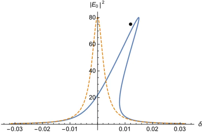
Fig. 1. Continuous wave bistability due to nonlinear Kerr tilt. Blue
solid line shows the resonance bistability for the intracavity power as a function of the detuning parameter, while the dashed orange line is the corresponding resonance in the absence of any non-linearity. The dot marks the detuning value at half the maximum power of the cavity soliton in Fig. 3. Parameters α = θ = 0.0025, 𝛾= 0.22 W−1m−1, L = 270π µm and P
in= 200 mW.
It is illuminating to consider the solution of Eqs.(11-12) for the intracavity power as a function of the detun-ing, while keeping the external pump power fixed. Fig-ure 1 shows how the Kerr nonlinearity introduces an in-tensity dependent tilt of the resonance that gives rise to the bistable behavior. In the mean-field approximation, there is only a single resonance corresponding to the pump mode present, but if multiple resonances are taken into ac-count, there is the possibility that the tilt of neighboring resonances becomes sufficiently large that they may, for
the same value of detuning, start to overlap with the pump mode resonance. A case of particular interest occurs when the neighboring resonances also overlap with the bistable response of the pump mode, that is, when the MI-stable low power branch is present. This case allows for the possi-bility of the creation of so-called super cavity solitons [46].
7 Cavity modulational instability
Modulational instability, i.e., the instability of the homo-geneous solution to time-periodic perturbations, is a phe-nomenon of fundamental importance for the generation of optical frequency combs. In fact, the parametric gain due to various four-wave mixing (FWM) processes is the underlying mechanism that allows for frequency conver-sion to occur in Kerr microresonators. A stable frequency comb can be seen as the end result of the cavity MI pro-cess, when parametric gain is able to balance and over-come the round-trip losses. Since MI is a pump degener-ate four-wave mixing process [26], it is also the primary comb generation mechanism for converting photons from the pump mode frequency into lateral sideband frequen-cies. The first set of primary sidebands that are gener-ated through MI will always have an equidistant frequency spacing owing to energy and momentum conservation, but subsequent sidebands generated via cascaded FWM of various combinations of comb line frequencies will not necessarily be equidistant or be an exact multiple of the cavity FSR [21].
Cavity MI of steady-state solutions of the LLE has some properties that are fundamentally different from those as-sociated with MI of a CW background solution of the NLSE (see e.g. Refs.[26, 47]). Cavity MI has an additional de-gree of freedom due to the detuning parameter, which may allow for phase matching between pump and side-bands waves to occur also in the normal dispersion regime [48, 49], contrary to the case of propagation in, for exam-ple, a length of optical fiber. Moreover, cavity MI is not an oscillatory instability but rather one where the unsta-ble eigenvalues are purely real, which permits the forma-tion of staforma-tionary dissipative structures such as periodic temporal patterns (also known as Turing patterns) and lo-calized cavity solitons [48, 50]. Besides the mean-field in-stabilities of the LLE, there are additional inin-stabilities that may occur in certain parameter regions where the dynam-ics should properly be modeled by using the Ikeda map formalism. These include so-called period doubling insta-bilities where the perturbation has a periodicity of two or
more round-trips, instead of a periodicity equal to the fun-damental round-trip period [51].
MI for the LLE (5) can be analyzed by a procedure where a perturbed solution of the form E(t, τ) = (|E0|+
u+ iv)eiArg{E0}is assumed, and the equation is linearized
around the steady-state CW solution. Separating real and imaginary parts, and investigating the coefficient matrix of the linear system obtained after applying the Fourier transform with respect to τ, leads to an eigenvalue prob-lem where the potentially unstable eigenvalues are given by [7, 8, 14, 19, 42]
λ= −α ±√︀(𝛾L|E0|2)2− (δ0− (β2L/2)ω2− 2𝛾L|E0|2)2.
(13) Perturbations will experience growth, and the CW solution will be modulationally unstable, whenever the real part of these eigenvalues is positive for some frequency. The insta-bility does not need to be seeded by a signal, but may grow from random noise fluctuations that are always present in the cavity.
From Eq.(13), it is possible to determine parameter regimes where instabilities may occur, and also obtain the threshold power needed for an instability to develop [15]. Cavity MI will not occur unless the parametric gain ex-ceeds the round-trip loss, which is in contrast to MI of the NLSE, which does not have a power threshold. Although the initial growth is exponential, the sideband growth rate will eventually saturate due to pump depletion, which per-mits the system to reach a stable equilibrium. However, far from all comb states are stable, and the majority of the pa-rameter space at high powers is dominated by an unstable regime of nonlinear development of MIs, where the comb spectrum is in a turbulent state of continuous fluctuations [52].
The previous stability analysis of the intracavity field is limited by the requirement that the magnitude of the perturbation should remain small. The dynamics of the growing perturbation beyond its initial linear stage and the subsequent depletion of the pump wave cannot be modeled by using the linearized approximation. However, additional insight into the dynamics can be found by con-sidering a fully nonlinear truncated three-wave model for the pump mode and the dominant sideband pair that ne-glects the influence of higher order sidebands [42, 43].
A truncated model can be obtained from Eq.(6) by con-sidering modes with indices µ = −1, 0, 1. This reduces the problem from an infinite dimensional system to just three coupled ODEs, with stationary comb states corresponding to fixed points given by the set of algebraic equations ob-tained by setting all time derivatives to zero. The ratio-nale for such a finite mode truncation is that a
substan-tial part of the total energy of the comb is contained in the pump mode and a small number of sidebands, which is certainly the case for many periodic temporal patterns that tend to have a triangularly shaped comb spectrum. Besides allowing for the identification of stationary states, trun-cated models are also able to give information about the comb stability. Particularly, it has been found that station-ary comb states that are predicted to be unstable by the analysis of the Jacobian matrix for the three-wave model, are generally also found to be unstable in numerical sim-ulations of the full model. Additionally, truncated mod-els allow for the identification of soft and hard excitation regimes, and have been used to predict the possibility for, and the range of, soft comb excitations in the normal dis-persion regime [42]. As an alternative, stationary solutions and comb stability can be ascertained numerically by us-ing, for example, a Newton root-finder [16]; however, this method does not easily permit one to search the entire so-lution space.
8 Boundary condition induced
modulational instability
In addition to the MI of the mean-field LLE, there are addi-tional instability mechanisms that occur due to the bound-ary conditions of the Ikeda map. This may be expected from the fact that the map with discrete boundary condi-tions is able to model multiple resonances in the cavity as previously discussed in relation to multistability. Partic-ularly, it is found that the boundary conditions may give rise to period doubling instabilities where the perturba-tion has a periodicity that is double that of the fundamen-tal round-trip time [49]. This corresponds to anti-resonant conditions where the nonlinear phase ϕ in Eq.(12) is an odd multiple of π, and it can be considered as an optical analog to a Möbius strip where the field needs two full laps of the resonator to recover its original phase.
Early work on the discrete map Eqs.(1-2) assumed a plane wave approximation, where the dispersion (or rather diffraction) effects of the cavity were neglected. In this case it is found that the intracavity field loses its stabil-ity through a period doubling cascade, which eventually leads to chaotic behavior [53]. However, this plane wave approximation is not well justified, since it was pointed out that the intracavity field is in fact more unstable with re-spect to periodic than to homogeneous perturbations [51]. With the exception of the low power threshold MI that is present in the mean-field models, most other instabilities tend to require quite large intracavity power levels for their
observation. These conditions are easily fulfilled for fiber-ring resonators, but they may also become important for microresonator devices with large nonlinearities or high finesse. In fact, large Kerr frequency mode shifts of up to 100 GHz have already been observed for high finesse silica microtoroids [2].
The general procedure for analyzing the stability of the map is relatively straightforward. First the perturbed so-lution is calculated by linearizing Eq.(2) around the ho-mogeneous CW solution. Then the perturbed solution is used in the map for the boundary condition Eq.(1) to de-termine the potentially unstable eigenvalues correspond-ing to a growcorrespond-ing perturbation. If absorption losses along the length of the resonator are neglected, and all losses are instead lumped together with coupling losses at the boundary, it is possible to analytically determine the un-stable eigenvalues, see Refs. [49, 51]. More generally, it is also possible to determine the MI gain by using numerical Floquet theory [46].
To use Floquet theory, one assumes a perturbed so-lution for Eq.(2) in the form E = [E0 + um(τ, z) +
ivm(τ, z)] exp[−αiz/2 + i𝛾(1 − e−αiz)|E
0|2/αi+ iArg{E0}],
where the perturbations um(τ, z) and vm(τ, z) are real
functions, and proceeds to linearize the wave equation around the CW solution. The real and imaginary parts of the resulting linear evolution equation for the side-bands will then each give an equation that can be Fourier transformed in order to obtain its frequency dependence. Specifically, one finds that the perturbation functions
wm(z) = [˜um(ω, z), ˜vm(ω, z)]T should satisfy the linear
ODE system dwm dz = [︃ 0 −(β2/2)ω2 (β2/2)ω2+ 2𝛾|E0|2e−αiz 0 ]︃ wm. (14) In the next step this system is numerically integrated for two independent initial conditions, for example, wm
1,2(0) =
[1, 0]T, [0, 1]T, as a function of both frequency and in-tracavity power to obtain the perturbed fields wm
1,2(L) at
the end of the round-trip. The boundary condition Eq.(1), which takes into account the coupling loss and the phase shifts experienced by the perturbations, is then applied to find the fields wm+11,2(0) that are to be compared with the ini-tial condition. The perturbed solution is finally assembled into a matrix [wm+11 (0), wm+12 (0)], and the eigenvalues are numerically calculated to determine the sideband stabil-ity. The stability criterion for the resulting system of differ-ence equations (or map) is that the real part of the eigen-values should be less than unity to avoid a growing pertur-bation.
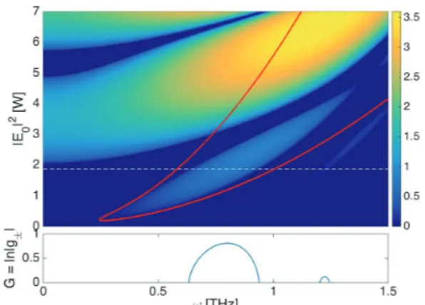
An example of parametric Ikeda map instabilities in the anomalous dispersion regime for parameters similar to the fiber-ring cavity of Ref. [54] is shown in Fig. 2. Also plotted as a red contour is the predicted range of modu-lational instability for the mean-field LLE. Multiple unsta-ble bands forming so-called resonance tongues are seen to appear at high intracavity powers. These bands corre-spond to MI obtained for either resonant or anti-resonant conditions, respectively, where the latter manifests itself through a change of sign of the perturbation at each round-trip. Following Ref. [49], we refer to them as CW-MI and P2-MI, respectively. P2-MI is most easily observed for normal dispersion resonators, where it is typically the instability with the lowest power threshold if the detuning has not been selected in order to phase match the CW-MI process.
Fig. 2. Parametric instability tongues of the Ikeda map for
anoma-lous dispersion. The red contour shows the predicted range of modulational instability for the LLE. Below a cross-section corre-sponding to the dashed line is shown with alternating CW-MI/P2-MI gain bands. Parameters corresponding to a fiber ring cavity with α= θ = 0.13, β2= −20 ps2km−1, 𝛾 = 1.8 W−1km−1, L = 380 m and δ0= 0.
9 Cavity solitons
Cavity solitons are of special importance for optical fre-quency combs. A cavity soliton is a localized pulse solu-tion of either the LLE or the Ikeda map, that corresponds to a mode-locked frequency comb with a comb line spac-ing of a sspac-ingle FSR. A temporal cavity soliton can be seen as a fixed point of a dynamical attractor [55] that represents a double balance between dispersive broadening and non-linear self-focusing, in combination with external pump driving and loss.
The first experimental demonstration of temporal Kerr cavity solitons was carried out in a fiber-ring cavity by Leo et al. in 2010 [54]. Since then, temporal cavity soli-tons have also been experimentally demonstrated in mi-croresonators with comb bandwidths spanning up to 2/3 of an octave [56]. A dissipative cavity soliton, an example of which is shown in Fig. 3, is a compound object con-sisting of a soliton pulse sitting on a constant background with a fixed pulse amplitude and temporal width that is set by the experimental parameters. Although there are no known exact analytical solutions of cavity solitons for the LLE, there exist various semi-analytical approximations. For example, if damping and driving are assumed to be small perturbations of the NLSE, then to the lowest order of approximation the single soliton solution of the LLE (5) can be explicitly written as (cf. Ref.[57])
E(t, τ) = −i √ θEin δ0 + √︂ 2δ0 𝛾Lsech (︃√︃ 2δ0 |β2|Lτ )︃ eiφ, (15) where the first term is the approximation for the CW back-ground solution and cos(φ) = 2α√︀2δ0/(π
√︀
𝛾Lθ|Ein|).
From Eq.(15), we can see that the soliton is phase locked with a certain phase offset to the pump, and that both the amplitude and width of the soliton are proportional to the square root of the detuning [58]. Bright cavity solitons are stable solutions existing for anomalous dispersion that are surprisingly robust to perturbations. A single soliton is characterized by a smooth spectral envelope, while multi-ple solitons lead to a modulated spectrum having an inter-ference pattern depending on the number of solitons and their relative positions [56].
Cavity solitons can be excited experimentally by tun-ing the pump laser frequency across the resonance from the blue detuned side, and then stopping the scan on the red detuned side whenever a staircase or step-like struc-ture in the output intensity is observed [39]. The soliton state is characterized by a transition from an MI induced unstable pattern state to a low phase-noise state where the comb exhibits a single narrowband beatnote centered at the FSR frequency. Since cavity soliton combs correspond to the circulation of a pulse with a periodicity of the round-trip time, they are analogous to frequency combs gener-ated by mode-locked lasers. Moreover, the soliton nature of the intracavity field solution allows for pulse compres-sion and spectral broadening techniques to be used, in or-der to extend the bandwidth of the generated spectrum, which can have important applications for the purpose of self-referencing [59]. Many aspects of cavity solitons such as excitation thorugh laser scanning, dispersive wave emission, and breathing behavior can also be seen and
have been directly confirmed by experiments in fiber cavi-ties, see for example, [40, 60, 61].
In addition to the cavity soliton solution of the LLE, there are also more energetic localized solutions present in the Ikeda map [46]. These so-called super cavity solitons are associated with multistable states, and can even coex-ist, for the same pump parameters, with the more familiar LLE cavity soliton. In particular, it has been numerically predicted that super cavity solitons should exist when-ever a multistable homogeneous state with three different branches is present. The background then corresponds to the MI stable low power branch, while the soliton peak power is close to twice the power of the highest branch. This can be understood from the fact that a soliton’s in-flexion points (zero of second derivative) should be close in power to that of the homogeneous branch solution, except for a small difference due to the relative phase offset (φ) be-tween the soliton and the background solution cf. Fig. 1. Super cavity solitons have only recently been predicted, and have not yet been experimentally observed. Since the bandwidth of these solutions can easily span more than an octave, super cavity solitons could be very interesting for wideband comb generation, in particular when com-bined with highly nonlinear materials and dispersion en-gineered resonators that are designed for enhanced spec-tral broadening. Time (ps) -0.1 -0.05 0 0.05 0.1 Power (W) 0 50 100 150 Frequency (THz) -60 -40 -20 0 20 40 60 Spectrum (dB) -60 -50 -40 -30 -20 -10 0
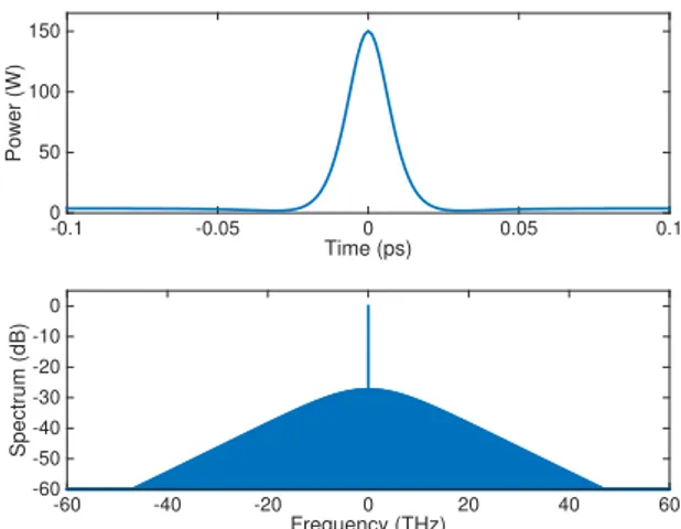
Fig. 3. Simulated intracavity intensity profile and normalized
spec-trum for a stationary temporal cavity soliton obtained from numeri-cal solution of the LLE (5). Same parameters as in Fig. 1 correspond-ing to a 200 GHz FSR silicon nitride microrcorrespond-ing with α = θ = 0.0025, β2= −3 ps2km−1, 𝛾 = 0.22 W−1m−1, L = 270π µm, δ0= 0.012 and Pin= 200 mW.
10 Conclusions
Microresonator devices can be used to generate ultra wide-band frequency combs, made up of phase coherent comb lines at an equidistant frequency spacing, that offer a wealth of potential applications. In this article, we have reviewed various formalisms currently used for model-ing the temporal dynamics and formation of such fre-quency combs. These formalisms include the Ikeda map, the frequency-domain modal expansion approach and the time-domain Lugiato-Lefever equation, all of which allow for the comb dynamics to be described, irrespective of the resonator morphology. The dispersive Ikeda map is the most general model available that permits combs to be described also in the high power regime. However, this generality comes at the cost of additional complexity and more computationally expensive numerical simulations when compared with mean-field models aimed at describ-ing combs that evolve slowly with respect to the round-trip time. This situation applies in practice to most microres-onator comb experiments: simulations based on both the Lugiato-Lefever equation and the coupled mode formal-ism are found to be in very good agreement with most ex-perimental observations.
We have further reviewed the stability properties that are of fundamental theoretical importance for the under-standing of different comb formation processes. The para-metric gain provided by the modulational instability of the pump mode wave is, in fact, the main comb generation mechanism when operating in the anomalous dispersion regime, with the instability occurring above a threshold power where the gain is able to overcome the round-trip loss. Owing to the extra degree of freedom provided by the detuning parameter, the cavity MI process may also become phase matched in the normal dispersion regime, which allows for the possibility of soft excitation comb generation for normal dispersion resonators. As the intra-cavity power increases, the influence of intra-cavity boundary conditions starts to become more important, which may lead to multistability and to the appearance of new insta-bilities that have a periodicity of either once or twice the fundamental round-trip time. Such higher-order instabili-ties and period doubling phenomena cannot be described using conventional mean-field models, and thus require use of the more general Ikeda map.
Most frequency comb experiments to date have fo-cused on the near-infrared part of the spectrum where transparent materials and pump sources are readily avail-able. Looking forward, we may expect a continued explo-ration and expansion into new wavelength regions such
as the mid-infrared [62], which has important applications for molecular spectroscopy. The use of materials such as silicon will be important for comb generation in this spec-tral range, and will require the use of models that are able to take into account the relevant new physics of these ma-terials, including effects such as multiphoton absorption and the associated free-carrier dynamics. Simultaneously we may also expect a push towards the miniaturization of existing comb sources and the integration of both mi-crorings and pump lasers together on a single photonic chip. Wideband comb generation from such integrated sources is currently not possible due to high pump power requirements, but the use of novel materials with large Kerr nonlinearities may be exploited in order to help re-duce the threshold power. Another promising avenue of exploration is the use of quadratic nonlinearities [63, 64], which, according to preliminary estimates, may increase the efficiency and reduce the pump power requirement for frequency comb generation even further.
Acknowledgment: This work was funded by the Swedish Research Council (grant no. 2013-7508) and the Ital-ian Ministry of University and Research (grant no. 2012BFNWZ2).
References
[1] T. J. Kippenberg, R. Holzwarth, and S. A. Diddams. Microresonator-Based Optical Frequency Combs. Science, 332(6029):555–559, April 2011.
[2] P. Del’Haye, T. Herr, E. Gavartin, M. L. Gorodetsky, R. Holzwarth, and T. J. Kippenberg. Octave Spanning Tun-able Frequency Comb from a Microresonator. Physical Review Letters, 107(6), August 2011.
[3] Yoshitomo Okawachi, Kasturi Saha, Jacob S. Levy, Y. Henry Wen, Michal Lipson, and Alexander L. Gaeta. Octave-spanning frequency comb generation in a silicon nitride chip. Optics letters, 36(17):3398–3400, 2011.
[4] Theodor Hänsch. Nobel Lecture: Passion for precision. Re-views of Modern Physics, 78(4):1297–1309, November 2006. [5] Scott B. Papp, Katja Beha, Pascal Del’Haye, Franklyn Quinlan,
Hansuek Lee, Kerry J. Vahala, and Scott A. Diddams. Microres-onator frequency comb optical clock. Optica, 1(1):10, July 2014.
[6] J. D. Jost, T. Herr, C. Lecaplain, V. Brasch, M. H. P. Pfeiffer, and T. J. Kippenberg. “Counting the cycles of light using a self-referenced optical microresonator,” Optica, 2(8):706, August 2015.
[7] Andrey Matsko, Anatoliy Savchenkov, Dmitry Strekalov, Vladimir Ilchenko, and Lute Maleki. Optical hyperparametric oscillations in a whispering-gallery-mode resonator: Thresh-old and phase diffusion. Physical Review A, 71(3), March 2005.
[8] Yanne K. Chembo and Nan Yu. Modal expansion approach to optical-frequency-comb generation with monolithic whispering-gallery-mode resonators. Physical Review A, 82(3), September 2010.
[9] Mark Oxborrow. Traceable 2-D Finite-Element Simulation of the Whispering-Gallery Modes of Axisymmetric Electromag-netic Resonators. IEEE Transactions on Microwave Theory and Techniques, 55(6):1209–1218, June 2007.
[10] Michael L. Gorodetsky and Aleksey E. Fomin. Geometrical the-ory of whispering-gallery modes. Selected Topics in Quantum Electronics, IEEE Journal of, 12(1):33–39, 2006.
[11] T. Hansson, D. Modotto, and S. Wabnitz. Analytical approach to the design of microring resonators for nonlinear four-wave mixing applications. Journal of the Optical Society of America B, 31(5):1109, May 2014.
[12] Yoshitomo Okawachi, Michael R. E. Lamont, Kevin Luke, Daniel O. Carvalho, Mengjie Yu, Michal Lipson, and Alexan-der L. Gaeta. Bandwidth shaping of microresonator-based frequency combs via dispersion engineering. Optics Letters, 39(12):3535, June 2014.
[13] Andrey B. Matsko and Vladimir S. Ilchenko. Optical resonators with whispering-gallery modes-part I: basics. Selected Topics in Quantum Electronics, IEEE Journal of, 12(1):3–14, 2006. [14] Kensuke Ikeda. Multiple-valued stationary state and its
insta-bility of the transmitted light by a ring cavity system. Optics Communications, 30(2):257 – 261, 1979.
[15] M. Haelterman, S. Trillo, and S. Wabnitz. Dissipative modu-lation instability in a nonlinear dispersive ring cavity. Optics Communications, 91(5-6):401–407, 1992.
[16] Stéphane Coen, Hamish G. Randle, Thibaut Sylvestre, and Miro Erkintalo. Modeling of octave-spanning Kerr frequency combs using a generalized mean-field Lugiato–Lefever model. Optics letters, 38(1):37–39, 2013.
[17] Matteo Conforti, Arnaud Mussot, Alexandre Kudlinski, and Stefano Trillo. Modulational instability in dispersion oscillat-ing fiber roscillat-ing cavities. Optics Letters, 39(14):4200, July 2014. [18] D. J. Kaup and A. C. Newell. Theory of nonlinear oscillating
dipolar excitations in one-dimensional condensates. Physical Review B, 18(10):5162, 1978.
[19] L. A. Lugiato and R. Lefever. Spatial dissipative structures in passive optical systems. Physical Review Letters, 58:2209– 2211, May 1987.
[20] A.B. Matsko, A.A. Savchenkov, W. Liang, V.S. Ilchenko, D. Sei-del, and L. Maleki. Mode-locked Kerr frequency combs. Optics Letters, 36(15):2845–2847, 2011.
[21] T. Herr, K. Hartinger, J. Riemensberger, C. Y. Wang, E. Gavartin, R. Holzwarth, M. L. Gorodetsky, and T. J. Kippenberg. Universal formation dynamics and noise of Kerr-frequency combs in microresonators. Nature Photonics, 6(7):480–487, June 2012. [22] A. A. Savchenkov, A. B. Matsko, W. Liang, V. S. Ilchenko,
D. Seidel, and L. Maleki. Kerr frequency comb generation in overmoded resonators. Optics express, 20(24):27290–27298, 2012.
[23] T. Herr, V. Brasch, J. D. Jost, I. Mirgorodskiy, G. Lihachev, M. L. Gorodetsky, and T. J. Kippenberg. Mode Spectrum and Tem-poral Soliton Formation in Optical Microresonators. Physical Review Letters, 113(12), September 2014.
[24] Yang Liu, Yi Xuan, Xiaoxiao Xue, Pei-Hsun Wang, Steven Chen, Andrew J. Metcalf, Jian Wang, Daniel E. Leaird, Minghao Qi, and Andrew M. Weiner. Investigation of mode coupling in
normal-dispersion silicon nitride microresonators for Kerr frequency comb generation. Optica, 1(3):137, September 2014. [25] Yanne K. Chembo and Curtis R. Menyuk.
Spatiotempo-ral Lugiato-Lefever formalism for Kerr-comb generation in whispering-gallery-mode resonators. Physical Review A, 87(5), May 2013.
[26] G.P. Agrawal. Nonlinear fiber optics, 5th Ed. Academic Press, New York, 2012.
[27] T. Hansson, D. Modotto, and S. Wabnitz. On the numerical simulation of Kerr frequency combs using coupled mode equa-tions. Optics Communications, 312:134–136, February 2014. [28] C. Milián and D.V. Skryabin. Soliton families and resonant
radiation in a micro-ring resonator near zero group-velocity dispersion. Optics Express, 22(3):3732, February 2014. [29] Michael R. E. Lamont, Yoshitomo Okawachi, and Alexander L.
Gaeta. Route to stabilized ultrabroadband microresonator-based frequency combs. Optics Letters, 38(18):3478, Septem-ber 2013.
[30] Changjing Bao, Lin Zhang, Andrey Matsko, Yan Yan, Zhe Zhao, Guodong Xie, Anuradha M. Agarwal, Lionel C. Kimerling, Jur-gen Michel, Lute Maleki, and Alan E. Willner. Nonlinear con-version eflciency in Kerr frequency comb generation. Optics Letters, 39(21):6126, November 2014.
[31] Maxim Karpov, Hairun Guo, Arne Kordts, Victor Brasch, Mar-tin Pfeiffer, Michail Zervas, Michael Geiselmann, and To-bias J. Kippenberg. Raman induced soliton self-frequency shift in microresonator Kerr frequency combs. arXiv preprint arXiv:1506.08767, 2015.
[32] R. Boyd. Nonlinear optics. Third Ed., Academic Press, 2008. [33] Austin G. Griflth, Ryan K.W. Lau, Jaime Cardenas, Yoshitomo
Okawachi, Aseema Mohanty, Romy Fain, Yoon Ho Daniel Lee, Mengjie Yu, Christopher T. Phare, Carl B. Poitras, Alexander L. Gaeta, and Michal Lipson. Silicon-chip mid-infrared frequency comb generation. Nature Communications, 6:6299, February 2015.
[34] Albert Schliesser, Nathalie Picqué, and Theodor W. Hänsch. Mid-infrared frequency combs. Nature Photonics, 6(7):440– 449, 2012.
[35] Lin Zhang, Anuradha M. Agarwal, Lionel C. Kimerling, and Ju-rgen Michel. Nonlinear Group IV photonics based on silicon and germanium: from near-infrared to mid-infrared. Nanopho-tonics, 3(4-5):247-268, 2013.
[36] Lianghong Yin and Govind P. Agrawal. Impact of two-photon absorption on self-phase modulation in silicon waveguides. Optics letters, 32(14):2031–2033, 2007.
[37] Q. Lin, O. J. Painter, and G. P. Agrawal. Nonlinear optical phe-nomena in silicon waveguides: modeling and applications. Optics Express, 15:16604, 2007.
[38] Tobias Hansson, Daniele Modotto, and Stefan Wabnitz. Mid-infrared soliton and Raman frequency comb generation in silicon microrings. Optics Letters, 39(23):6747, December 2014.
[39] T. Herr, V. Brasch, J. D. Jost, C. Y. Wang, N. M. Kondratiev, M. L. Gorodetsky, and T. J. Kippenberg. Temporal solitons in optical microresonators. Nature Photonics, 8(2):145–152, December 2013.
[40] Kathy Luo, Jae K. Jang, Stéphane Coen, Stuart G. Murdoch, and Miro Erkintalo. Spontaneous creation and annihilation of temporal cavity solitons in a coherently driven passive fiber resonator. Optics Letters, 40(16):3735, August 2015.
[41] Ryan K. W. Lau, Michael R. E. Lamont, Yoshitomo Okawachi, and Alexander L. Gaeta. Effects of multiphoton absorption on parametric comb generation in silicon microresonators. Optics Letters, 40(12):2778, June 2015.
[42] T. Hansson, D. Modotto, and S. Wabnitz. Dynamics of the modulational instability in microresonator frequency combs. Physical Review A, 88(2), August 2013.
[43] A. B. Matsko, A. A. Savchenkov, V. S. Ilchenko, D. Seidel, and L. Maleki. Hard and soft excitation regimes of Kerr frequency combs. Physical Review A, 85(2), February 2012.
[44] A. B. Matsko, A. A. Savchenkov, and L. Maleki. Normal group-velocity dispersion Kerr frequency comb. Optics Letters, 37(1):43–45, 2012.
[45] J. A. Jaramillo-Villegas, X. Xue, P.-H. Wang, D. E. Leaird, and A. M. Weiner. “Deterministic single soliton generation and compression in microring resonators avoiding the chaotic region.” Optics Express, 23(8):9618, April 2015.
[46] Tobias Hansson and Stefan Wabnitz. Frequency comb genera-tion beyond the Lugiato–Lefever equagenera-tion: multi-stability and super cavity solitons. Journal of the Optical Society of America B, 32(7):1259, July 2015.
[47] S. Trillo and Stefan Wabnitz. Dynamics of the nonlinear modu-lational instability in optical fibers. Optics letters, 16(13):986– 988, 1991.
[48] Marc Haelterman, S. Trillo, and S. Wabnitz. Additive-modulation-instability ring laser in the normal dispersion regime of a fiber. Optics letters, 17(10):745–747, 1992. [49] Stéphane Coen and Marc Haelterman. Modulational instability
induced by cavity boundary conditions in a normally disper-sive optical fiber. Physical review letters, 79(21):4139, 1997. [50] Aurelien Coillet, Irina Balakireva, Remi Henriet, Khaldoun
Saleh, Laurent Larger, John M. Dudley, Curtis R. Menyuk, and Yanne K. Chembo. Azimuthal Turing Patterns, Bright and Dark Cavity Solitons in Kerr Combs Generated With Whispering-Gallery-Mode Resonators. IEEE Photonics Jour-nal, 5(4):6100409, August 2013.
[51] D. W. McLaughlin, J. V. Moloney, and A. C. Newell. New class of instabilities in passive optical cavities. Physical review letters, 54(7):681, 1985.
[52] P. Parra-Rivas, D. Gomila, M. A. Matías, S. Coen, and L. Gelens. Dynamics of localized and patterned structures in the Lugiato-Lefever equation determine the stability and shape of optical frequency combs. Physical Review A, 89(4), April 2014. [53] K. Ikeda, H. Daido, and O. Akimoto. Optical turbulence
-Chaotic behavior of transmitted light from a ring cavity. Physi-cal Review Letters, 45:709–712, September 1980.
[54] François Leo, Stéphane Coen, Pascal Kockaert, Simon-Pierre Gorza, Philippe Emplit, and Marc Haelterman. Temporal cavity solitons in one-dimensional Kerr media as bits in an all-optical buffer. Nature Photonics, 4(7):471–476, May 2010.
[55] D. W. Mc Laughlin, J. V. Moloney, and A. C. Newell. Solitary waves as fixed points of infinite-dimensional maps in an opti-cal bistable ring cavity. Physiopti-cal review letters, 51(2):75, 1983. [56] V. Brasch, M. Geiselmann, T. Herr, G. Lihachev, M. H. P.
Pfeif-fer, M. L. Gorodetsky, and T. J. Kippenberg. “Photonic chip-based optical frequency comb using soliton Cherenkov radia-tion.” Science, 351(6271):357-360, January 2016.
[57] Stefan Wabnitz. Suppression of interactions in a phase-locked soliton optical memory. Optics letters, 18(8):601–603, 1993.
[58] Stéphane Coen and Miro Erkintalo. Universal scaling laws of Kerr frequency combs. Optics Letters, 38(11):1790, June 2013. [59] Tobias Herr, Michael L. Gorodetsky, and Tobias J. Kippenberg.
Dissipative Kerr solitons in optical microresonators. arXiv preprint arXiv:1508.04989, 2015.
[60] François Leo, Lendert Gelens, Philippe Emplit, Marc Haelter-man, and Stéphane Coen. Dynamics of one-dimensional Kerr cavity solitons. Optics Express, 21(7):9180, April 2013. [61] Jae K. Jang, Miro Erkintalo, Stuart G. Murdoch, and Stéphane
Coen. Observation of dispersive wave emission by temporal cavity solitons. Optics Letters, 39(19):5503, October 2014. [62] C. Y. Wang, T. Herr, P. Del’Haye, A. Schliesser, J. Hofer,
R. Holzwarth, T. W. Hänsch, N. Picqué, and T. J. Kippenberg. Mid-infrared optical frequency combs at 2.5 µm based on crys-talline microresonators. Nature Communications, 4:1345, January 2013.
[63] Iolanda Ricciardi, Simona Mosca, Maria Parisi, Pasquale Maddaloni, Luigi Santamaria, Paolo De Natale, and Maurizio De Rosa. Frequency comb generation in quadratic nonlinear media. Physical Review A, 91(6), June 2015.
[64] F. Leo, T. Hansson, I. Ricciardi, M. De Rosa, S. Coen, S. Wab-nitz, and M. Erkintalo. “Walk-Off-Induced Modulation In-stability, Temporal Pattern Formation, and Frequency Comb Generation in Cavity-Enhanced Second-Harmonic Generation.” Physical Review Letters, 116(3):033901, January 2016.