Fluid Dynamics Simulations on Multi-GPU Systems

UNIVERSITÀ DEGLI STUDI DI CATANIA

Facoltà di Scienze Matematiche, Fisiche e Naturali

Dottorato di Ricerca in Informatica

FLUID DYNAMICS SIMULATIONS

ON MULTI-GPU SYSTEMS

Eugenio Rustico

A dissertation submitted in partial fulfillment of the requirements

for the degree of “Research Doctorate in Computer Science”

Coordinator

Chiar.mo Prof. Domenico Cantone

Acknowledgements

This thesis would not have been possible without the help, encouragement, pa-tience and love of my family.

Thank you. You are the start and the goal of my path.

I would like to thank all my friends and colleagues of IPLab and DMI and in particular prof. Giovanni Gallo, for his precious tips and advices.

A special thank goes to the friends and colleagues of the INGV Catania. I would like to thank especially Dr. Ciro Del Negro for his help, esteem, assistance and trust.

Many people helped me growing professionally and culturally along the path of the Ph.D. In particular, I owe my deepest gratitude to prof. Robert A. Dalrymple, prof. Alexis Hérault and Dr. Giuseppe Bilotta. Your help was more than priceless. Developers and dreamers all around the world made possible GNU/Linux, LA_{TEX, Inkscape and a huge number of high quality tools I could use for free. I feel}

Contents

Table of Contents 2

1 Introduction 7

1.1 Contribution . . . 8

I

GPU computing

10

2.2 From hacking to CUDA . . . 13

2.3 Numerical precision . . . 16

2.4 Recent advances . . . 17

3 CUDA 19 3.1 Compute Capabilities. . . 20

3.2 Multiprocessors . . . 21

3.3 Kernels, warps, blocks . . . 22

3.4 Memory types . . . 24

3.5 Coalescence . . . 25

3.6 Contexts . . . 27

3.7 Streams . . . 28

CONTENTS 3 3.9 Libraries . . . 31 4 Multi-GPU computing 32 4.1 Motivation . . . 32 4.2 Naïve approach . . . 33 4.3 Subproblems inter-dependence . . . 34 4.4 Overhead . . . 34 4.5 Speedup metrics. . . 35 4.5.1 Amdahl’s law . . . 36 4.5.2 Gustafson’s law . . . 37 4.5.3 Karp–Flatt metric . . . 38 4.6 Linear overhead . . . 38 4.7 Timeline profiling . . . 40 4.8 Testbed . . . 43 4.8.1 MAGFLOW . . . 43 4.8.2 GPUSPH . . . 43 4.8.3 Hardware . . . 44

II

The MAGFLOW simulator

45

5.2 Model. . . 47

5.3 Single-GPU MAGFLOW . . . 48

6 Multi-GPU MAGFLOW 51 6.1 Splitting the problem . . . 51

6.2 Hiding row transfers . . . 54

CONTENTS 4

6.4 From serial to parallel code . . . 57

6.5 Preliminary performance analysis . . . 58

6.6 Load balancing . . . 61

6.7 Interface . . . 62

6.8 Results . . . 63

III

The GPUSPH simulator

66

7.1.1 SPH for derivatives . . . 69

7.1.2 SPH for Navier Stokes . . . 70

7.1.3 Integration . . . 71

7.2 Related work. . . 72

7.3 Single-GPU GPUSPH . . . 74

7.3.1 Kernels . . . 74

7.3.2 Fast neighbor search . . . 75

7.3.3 Memory requirements . . . 76

7.3.4 Speedup . . . 78

8 Multi-GPU GPUSPH 79 8.1 Splitting the problem . . . 79

8.2 Split planes . . . 81

8.3 Subdomain overlap . . . 84

8.4 Kernels . . . 84

8.5 Hiding slice transfers . . . 86

8.6 Simulator design . . . 88

8.7 Performance metrics . . . 89

CONTENTS 5 8.9 Numerical precision . . . 93 8.10 Load balancing . . . 93 8.11 Final results . . . 98

IV

Conclusions

105

CONTENTS 6

Whether you think you can, or you think you can’t - you’re right. Henry Ford

Chapter 1

Introduction

The realistic simulation of fluid flows is fundamental in a number of fields, from entertainment to engineering, from astrophysics to city planning. In particular, there are a number of applications related to civil protection: simulating a tsunami, an ash cloud or a lava flow, for example, has an important role both in disaster prevention and damage mitigation.

The Sezione di Catania of the Istituto Nazionale di Geofisica e Vulcanologia (INGV-CT) is a leading research center in the fields of natural hazard assessment and lava flow simulation. In the past 10 years, in collaboration with the Univer-sity of Catania, two lava simulators have been developed: one uses a Cellular Automaton (CA) approach, while the other is based on the Smoothed Particle Hy-drodynamics (SPH) method.

The CA simulator, called MAGFLOW, has been widely used for hazard as-sessment and forecasting, as it is capable of simulating lava flow with Bingham rheology on an arbitrary DEM (Digital Elevation Model, a 2D representation of a 3D topography). The SPH-based one, called GPUSPH, has been recently devel-oped for its capability to model a fluid in a truly three-dimensional environment while simulating complex phenomena such as solid-fluid interaction, crust forma-tion and tunneling.

1. Introduction 8

Such complex and flexible simulators come at the price of a high level of com-plexity and a significant computational cost. The simulation of an eruption, to be useful in any application (ranging from scenario forecasting to statistical analysis, from the validation of the model itself to its sensitivity analysis) should take sig-nificantly less time than the simulated event; an efficient implementation is thus needed for any practical application.

Among the possible high-performance computing solutions available, GPU computing is nowadays one of the most cost-effective in terms of Watt per FLOPS and nevertheless one of the most powerful ones. For this reason, the MAGFLOW simulator has been ported for the execution on GPU while GPUSPH, as the name suggests, has been natively written with GPU computing in mind. This has greatly improved the performance of MAGFLOW with respect to the correspondent CPU implementation and allowed GPUSPH to complete a simulation in a reasonable time (faster than 1:1). A multi-GPU version of both simulators has been recently developed to increase the performance and, for GPUSPH, to allow simulations that would not fit the memory of a single GPU.

1.1

Contribution

The subject of this thesis is the original multi-GPU implementation of both MAGFLOW and GPUSPH simulators. As later explained, it is not trivial to ex-ploit more than one device simultaneously to solve complex problems like SPH or cellular-automaton based fluid simulations. We had to overcome several technical and model-related challenges mainly due to the locality required by the problem computational units (cells, particles) and to the latencies introduced by using off-CPU devices. The resulting multi-GPU simulators allow faster simulations and enable GPUSPH to simulate sets of particles bigger than a single GPU could fit. To the best of our knowledge, these are the first multi-GPU Cellular-Automaton

1. Introduction 9

based lava simulator and the first multi-GPU Navier-Stokes SPH fluid simulator. In the first parts we introduce the concepts of GPU computing, GPGPU, multi-GPU and CUDA. The second part is dedicated to the MAGFLOW simulator; the single-GPU version is briefly described and then the multi-GPU implementation is introduced. A similar structure is used in the third part, where the single- and multi-GPU implementations of GPUSPH are described. Finally, in the fourth part, the results are briefly discussed.

The results presented in sections 6.8 and8.11 show a performance gain almost

linear with the number of GPUs used. The simulators have been tested for using up to 6 GPUs simultaneously and the execution times differ from the ideal ones only by a small cost function which is itself linear with the number of GPUs.

Two load balancing approaches have been designed, implemented and tested: an a priori balancing for MAGFLOW and an a posteriori one for GPUSPH. The former dynamically changes according to the bounding box variations of the sim-ulated fluid. The latter one makes GPUSPH perform steadily even in very asym-metric simulations, where a static split would perform about 50% worse.

The performance results are formally analyzed and discussed. While the re-sults are close to the ideal achievable speedups, some future improvements are hypothesized and open problems are mentioned.

Part I

Chapter 2

The Graphics Processing Unit

A GPU (Graphics Processing Unit) is a microprocessor specialized in graphics-related operations. GPUs have been traditionally used to offload and accelerate graphic rendering from the CPU by providing direct hardware support for com-mon 2D and 3D graphics primitives.

The market of videogames has probably been the most important pushing fac-tor towards faster and faster GPUs, which are nowadays incredibly faster than CPUs in parallel, arithmetic-intensive tasks like matrix manipulations and coordi-nate projections.

Figure 2.1: Screenshots of Castle Wolfenstein (1981), Wolfenstein3D (1992), Return to Castle Wolfenstein (2009) and Wolfenstein (2011).

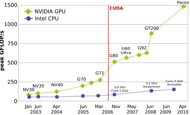
Fig. 2.2 shows the trend of peak computational power of CPUs vs. GPUs,

from 2003 to 2010, with an always increasing gap. However, as the GPUs are typically many-cores with a lower clock rate, it is more difficult to reach the peak value of a GPU, as not all the computational problems can be split in independent, parallel tasks. The red vertical line marks the introduction of the CUDA GPGPU

2. The Graphics Processing Unit 12 computing platform. NVIDIA GPU Intel CPU p e a k G F L OP /s 1000 750 500 250 0 1500 NV30NV35 NV40 G70 G71 G80 G80 Ultra G92 GT200 Fermi 3.2 Ghz Harpertown 3.0 Ghz Core 2 Duo Core i7-920 Arrandale

Jan Jun Apr Jun Mar Nov May Jun

2003 2004 2005 2006 2007 2008 2009Jun 2010Apr CUDA

Figure 2.2: Trend of theoretical computational power of CPUs and GPUs, 2003-2010

2.1

Birth of GPGPU

In 2001 NVIDIA released the first chip capable of programmable shading, i.e. a GPU with which it was possible to customize the arithmetic pipeline to obtain very sophisticated surface renderers. Programmable shading later became a standard GPU feature also for other brands.

While programmable shaders were meant to be used for graphical purposes, there was a growing interest in using graphic cards also as general-purpose stream processing engines [78, 33]. Engineers and scientists started using them for

non-graphical calculations by mapping a non-graphic problem to a graphic one and letting the GPU compute it. To cite a few examples, in [12] a programmable shader

is used to simulate the behavior of a flock; in [34] pixel shaders are used for both

visualization and evolution of Cellular-Automaton based simulations; in [50] a

2. The Graphics Processing Unit 13

The possibility to use a specialized microprocessor for generic purpose prob-lems marked the beginning of the GPGPU paradigm, where the acronym GPGPU stands for General-Purpose Graphics Processing units. The hack of mapping a non-graphic problem to a non-graphic one, however, was complex and cumbersome, and required the programmer to know many hardware details as well as to code using the hardware assembly language.

2.2

From hacking to CUDA

In 2007 NVIDIA released CUDA (acronym for Compute Unified Device Architec-ture), a hardware and software architecture with explicit support for general pur-pose programmability. The ground-breaking feature of CUDA was the possibility to code for the GPU using an extension of the C programming language1

.

1 f o r (i= 0 ; i< 4 0 9 6 ; i+ + ) 2 c p u _ a r r a y[i] = i;

Listing 2.1: Array initialization in C++ for serial execution on the CPU.

1 # d e f i n e B L K S I Z E 64 2 . . . 3 _ _ g l o b a l _ _ v o i d i n i t _ k e r n e l(i n t* g p u P o i n t e r) { 4 i n d e x = b l o c k D i m.x*b l o c k I d x.x + t h r e a d I d x.x; 5 g p u P o i n t e r[i n d e x] = i n d e x; 6 } 7 . . . 8 i n i t _ k e r n e l< < < 4 0 9 6 /B L K S I Z E, B L K S I Z E > > >(g p u _ a r r a y) ;

Listing 2.2: Array initialization in CUDA C for parallel execution on the GPU. 1

CUDA C is C extended with a few GPU-specific keywords and implicit library calls, but with some limitations like no possibility to call external libraries, no direct CPU memory access, no recursion (this limit has been overcome in recent versions), etc.

2. The Graphics Processing Unit 14

Listing 2.1 is an example of serial array initialization on the CPU, in C; listing 2.2is an equivalent CUDA C array initialization for parallel execution on the GPU.

Also ATI, NVIDIA’s main competitor, released soon after a GPGPU architecture called Stream; instead of a high-level language, Stream requires to program the GPU with a low-level assembly language.

A modern GPU typically hosts more cores then a CPU, up to a one thousand, and runs with a slightly lower clock rate. This setting is ideal to implement a SIMD (Single Instruction Multiple Data) paradigm, where a series (stream) of instructions is executed in parallel on multiple data. Fig. 2.4is a graphical representation of the

SISD (Single Instruction Single Data), SIMD and stream processing approaches.

Figure 2.3: SISD (Single Instruction Single Data), SIMD (Single Instruction Multiple Data) and Stream Processing.

From a programmer’s perspective, a GPU may be seen as an external com-puter with its own RAM memory and processors; the typical workflow consists in transferring the input data from the CPU memory to the GPU memory, requesting a computation and transferring back the resulting output. Following a common convention, we will refer to the GPU and its RAM as device and to the CPU and its memory as host.

2. The Graphics Processing Unit 15

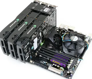
Some classes of problems can be solved much faster on GPUs and achieve speedups of two orders of magnitude with respect to the correspondent CPU im-plementations, as long as they expose a high level of parallelism on a fine data granularity. The price of such a speed benefit is a slight change in the program-ming logic or, sometimes, a complete rewrite of the computational core. The high cost-effectiveness of GPU-based solutions is, however, the main breakthrough of this phenomenon. A single workstation with modern consumer GPUs easily reaches the theoretical speed of one TFLOPS (1012 Floating Point Operations Per Second), while costing less than ¤1, 000 and consuming less than 800W.

Figure 2.4: A consumer-level multi-GPU workstation reaching the theoretical speed of one TFLOPS

Even devices dedicated to scientific computing like the NVIDIA Tesla boards, which share the chipset with the consumer-level GPUs, are still a very cost-effective solution and have been recently used also in supercomputing environments. In may, 2010 a hybrid CUDA-enabled Chinese supercomputer called Nebulae reached the theoretical peak performance of 2.98 PFlops, ranking first in the list of the most powerful commercial systems in the world, and second by means of actual measured performance [53]. Later in 2010 another GPU-based Chinese

supercom-puter, Tianhe-1A, ranked first in the TOP500 list with an actual performance of 2.57 PFlops. In June 2011 another GPU-based supercomputer called TSUBAME 2.0

2. The Graphics Processing Unit 16

entered the top ten; in November 2011 Nebulae, Tianhe-1A and TSUBAME 2.0 still rank among the top 5 most powerful supercomputers in the world.

The cost-effectiveness and the ease of utilization of modern GPUs, along with the wide spread of GPU computing even outside the commercial and academic world, led some to claim that the GPU Computing Era has begun [62]. It is worth

mentioning, however, that some others criticized the excess of enthusiasm for GPGPU and proved that a well-tuned CPU implementation, optimized for exe-cution on recent multi-core processors, often reduces the flaunted 100× speedup reported by many works [51].

2.3

Numerical precision

Another little price of porting an application to GPGPU, apart from the effort of a little re-engineering, regards numerical precision.

It is useful to recall that floating point arithmetic introduces a systematic er-ror that is important to take into account and mitigate through the use of specific numerical techniques [25]. For example, a common and underestimated source of

error is the non-commutativeness of floating point operations: this is particularly visible when the numbers involved differ by orders of magnitude such as, for ex-ample, when adding alternatively very large numbers and numbers very close to zero. Different implementations of the same algorithm may result in a little change in the order of additions, and if the method is not numerically stable these errors will propagate and amplify, becoming “mysterious” big changes in the output. This is a common issue in GPU computing, as porting a software for the execution on a many-core GPU often requires slight changes in the order of computations and the output may not match with the one produced with the reference serial code. Techniques such as the Kahan summation [46] can reduce the numerical

2. The Graphics Processing Unit 17

levels of accuracy.

Another potential cause of differences between a CPU and a GPU implemen-tation relies in the hardware precision. Among the formats defined in IEEE 754 standard for floating point arithmetic [44], single precision and double precisions are

the most common ones. Their length is respectively 32 and 64 bits and their cor-respondent C/C++ types are float and double. While most desktop and work-station CPUs have had hardware support for both types since the ’90s, GPUs have, until recently, only featured hardware support for single precision, sometimes of-fering the possibility to emulate double precision (in NVIDIA cards, an emulated double precision operation is 8×slower than a hardware single precision one). As the computations performed on the GPU were mainly devoted to compute pixel coordinates for graphics, single precision was totally acceptable. Because of the increased request for numerical precision, especially in GPGPU scientific comput-ing, ATI and NVIDIA afterwards recently introduced on-chip support for double precision also in GPU cards. Most non high-end cards, however, still use single precision as default. This is an issue to take into account for applications requiring double precision.

2.4

Recent advances

Both NVIDIA’s CUDA and ATI’s Stream run on specific GPU hardware, with prac-tically no interoperability between the two. Because of the growing interest for parallel computing and the wider range of hardware available, an architecture-independent parallel computing platform, OpenCL, was proposed in 2008 by Ap-ple and released in 2009 as the result of a collaboration with AMD, IBM, Intel, and NVIDIA [28].

OpenCL was designed to offer an abstraction layer between the applications and the underlying hardware, allowing an application to be transparently executed

2. The Graphics Processing Unit 18

on heterogeneous hardware (GPUs as well as multicore CPUs and other hardware). The language is derived from C99 and the API is similar to the low-level CUDA C API. Coding in OpenCL is in general more complex than CUDA C, due to the wider variety of hardware on which it runs, but does not force the programmer to bind to a specific hardware class or brand.

We started approaching the GPGPU paradigm in 2007, when CUDA was the only platform allowing for generic purpose programmability in a C-like language. For this reason, our GPU-enabled simulators are at moment CUDA-based, but we are considering the possibility to port our softwares to the OpenCL platform in a near future.

Chapter 3

CUDA

As mentioned before, the CUDA platform consists of a hardware and a software part. The hardware required to run a CUDA routine can be found quite easily as any graphic card produced by NVIDIA since the release of the GeForce 8 series (2006) is CUDA-capable1

; many old PC’s are therefore already CUDA-enabled, while it is possible to buy a low-end CUDA-enabled card with less than ¤50.

On the software side, a CUDA application relies on two layers: a CUDA-enabled video driver, which is capable of communicating with the graphic card at the operative system level, and the CUDA Toolkit, which is a set of shared li-braries, tools and bindings needed to compile the code for the GPU and integrate it into a “normal” application. There are two different programming interfaces to the CUDA runtime libraries: the low-level API, that exposes to the programmer a higher number of structures to access and use a GPU, and the high-level API, that automatizes the most common operations. The latter one allows a programmer to drive a GPU with just a few C functions that closely follow the naming convention and parameter order of similar functions from the C standard library.

1

The NVIDIA website states that CUDA-enabled GeForce cards are “GeForce 8, 9, 100, 200, 400-series, 500-series GPUs with a minimum of 256MB of local graphics memory”.

3. CUDA 20

3.1

Compute Capabilities

enable applications are in general backwards-compatible with all CUDA-enabled hardware, but new generation cards may offer additional features not supported in previous devices. The set of capabilities of a given generation has version number referred as compute capabilities and it is 2.1 in the latest generation cards (Fermi architecture) as of this writing. As an example, one needs a card with at least compute capability 1.1 to use atomic operations and 1.3 for hardware support for double precision. One could define the compute capabilities as the hardware version of a card, the major number referring to the generation; the Toolkit has an independent version number, which recently has arrived to 4.0.

The toolchain used to implement a function for the GPU consists of the follow-ing steps:

1. Write the function (kernel) to be executed on the GPU in CUDA C with any IDE/text editor, even mixing CPU and GPU functions in the same source files;

2. Compile the files containing GPU code with the Toolkit compiler (nvcc); 3. nvcc transparently compiles the GPU code into the card’s assembly2, lets a

predifined C/C++ compiler (gcc in Unix-based systems) compile the CPU code and links together the GPU and CPU binary objects.

It is possible to run the resulting application on any hardware with compute capability equal or greater than the target one, as long as a possibly up-to-date video driver is installed. From the programmer’s perspective, the only change from the usual toolchain is using nvcc in place of gcc.

2

nvcccompiles the GPU code into both PTX (a proprietary assembly which abstracts from the hardware, always forward compatible) and CUBIN (the actual binary code for the GPU, forward-compatible only with CUDA architectures of the same compute capability major version); when a CUDA application is run, it loads the CUBIN to the GPU, if compatible, or does a just-in-time compilation to produce a proper CUBIN from the PTX.

3. CUDA 21

3.2

Multiprocessors

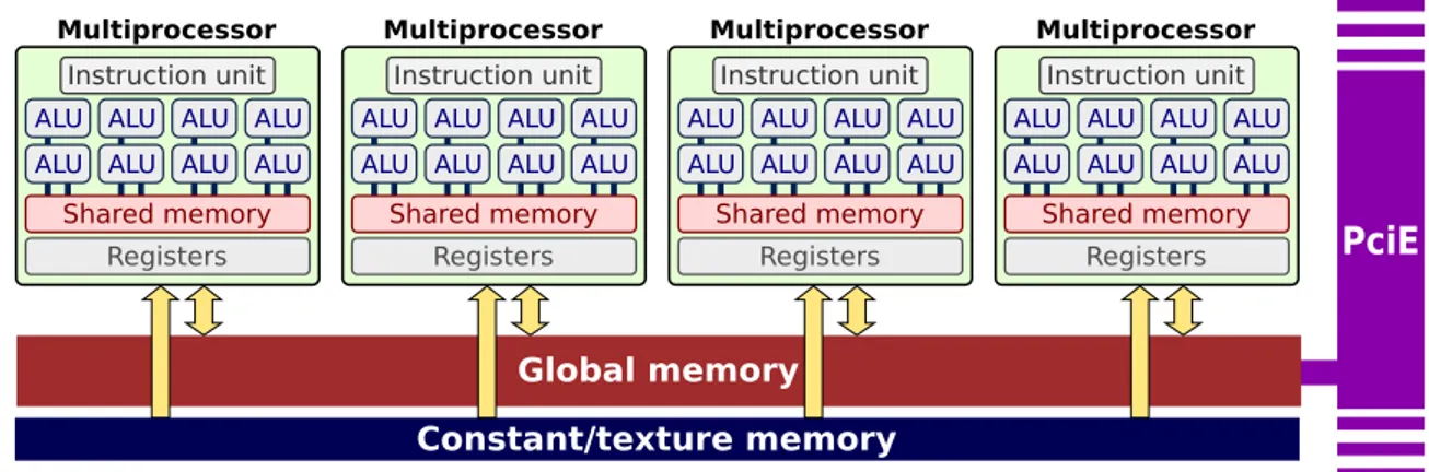
Although programming with CUDA platform does not require the knowledge of the details fo the underlying hardware, the way GPU threads are launched and the characteristics of features like shared memory strongly reflect the way GPU cores and memory banks are organized in the card. It is therefore advisable to learn at least the basic principles in order to be able to fully exploit the hardware capabilities.

Similarly to other NVIDIA and non-NVIDIA GPUs, CUDA-enabled cards host one or more SIMD multiprocessors each embodying several computational cores, for a total of tens or even hundreds of cores. Recent cards such as the GTX 590 host up to 1024 CUDA cores, for a total 3 billion transistors. More specifically, each multiprocessor hosts 8 to 32 ALUs and one instruction unit that decodes one instruction at a time to be executed in lockstep3

by multiple threads. Distinct multiprocessors execute thread batches (called warps in CUDA terminology) in parallel but independently from each other.

Shared memory

Registers ALU ALU ALU ALU ALU ALU ALU ALU

Instruction unit

Multiprocessor

Shared memory

Registers ALU ALU ALU ALU ALU ALU ALU ALU

Instruction unit

Multiprocessor

Shared memory

Registers ALU ALU ALU ALU ALU ALU ALU ALU

Instruction unit

Multiprocessor

Shared memory

Registers ALU ALU ALU ALU ALU ALU ALU ALU

Instruction unit

Multiprocessor

Global memory Constant/texture memory

PciE

Figure 3.1: Schematic representation of how GPU cores are grouped into multiprocessors and linked to shared and global memory banks.

Recent consumer-level cards host up to 1.5Gb GDDR5 memory and support hardware double precision; high-end cards like Tesla host larger RAM memory

3

Here intended in the parallel computing meaning, as the same instruction is performed syn-chronously by different cores, not in the meaning of redundant computing.

3. CUDA 22

with optional ECC support. There are other memory resources, such as a global constant memory (cached, read-only) and textures (spatially cached, read only until rebound, although more recent hardware allows writing to texture too). Each multiprocessor also hosts a bank of shared memory, directly accessible by all ALUs and much faster than global memory (RAM). Shared memory, however, has a limited size (16-48Kb) and its temporal scope is limited to the execution of one block. Because of its high speed and low latency, shared memory is often used to exchange data between threads of the same block, handle race conditions or simply avoid multiple reads in global memory by storing them in a shared buffer. It is up to the programmer to carefully evaluate which kind(s) of memory it is convenient to exploit for a specific problem and how to access them.

3.3

Kernels, warps, blocks

We already referred to the series of instructions to be executed on a GPU as kernel; we can see a kernel as a function compiled for the GPU and meant to be executed in parallel on multiple data streams (SIMD).

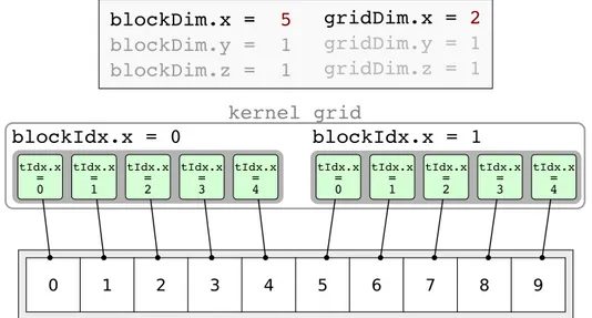
The instance of a kernel is called GPU thread, or simply thread when the context does not allow for any ambiguity. Kernels are instantiated in parallel threads and threads are grouped into blocks with one, two or three dimensions; blocks are in turn arranged in a one-, two- or (only with the most recent compute capabilities) three-dimensional grid. The block and grid sizes are up to the programmer, and can be decided at runtime. The position of a kernel in a block and the one of the block in the grid, as well as the block and grid sizes, are available inside the kernel in the form of implicitly defined variables, so that it is possible for each thread to compute the address of the data to be accessed.

Blocks have a size limit that may depend on the underlying architecture and this limit is in general lower than the number of threads a typical application

3. CUDA 23 blockIdx.x = 0 blockIdx.x = 1 0 1 2 3 4 5 6 7 8 9 0 tIdx.x = 1 tIdx.x = 2 tIdx.x = 3 tIdx.x = 4 tIdx.x = 0 tIdx.x = 1 tIdx.x = 2 tIdx.x = 3 tIdx.x = 4 tIdx.x = blockDim.x = 5 blockDim.y = 1 blockDim.z = 1 gridDim.x = 2 gridDim.y = 1 gridDim.z = 1 kernel grid

Figure 3.2: Simple example of two one-dimensional blocks each assigned to a portion of a global array.

Figure 3.3: Example thread indexing on a 2D grid of 2D blocks.

would instantiate. This means that grouping the threads into blocks is not just possible, but often necessary, and it is related to the hardware structure.

Each block is assigned to a multiprocessor which, as already mentioned, exe-cutes multiple threads simultaneously (a warp). When the number of threads is greater than the number of cores, a minimal context switch is executed to let all threads complete. When a thread issues a memory request that may take several cycles (e.g. accessing a word in the RAM memory of the card takes about 400 clock

3. CUDA 24

cycles in 2.0 hardware, 800 clock cycles in previous cards) the context switch lets other threads execute while one is waiting for the resulting data. Thus, instanti-ating more threads than cores (and, in general, issuing enough computations to saturate the hardware) leads to a higher throughput as time-consuming memory requests are covered by computations.

Another time-consuming factor is divergency. When two or more threads of the same warp need to execute different instructions because of a branch divergence, those operations are serialized. The programmer should take care to avoid as much as possible that threads of the same warp diverge.

3.4

Memory types

There are several kinds of memory available on the device, each with specific features and limits:

• Registers: R/W, very fast, not cached, local to each thread; it is not possible to access them directly. The total number of registers on a card is fixed and it is divided among the threads; this limits the complexity of kernels and the number of concurrent threads.

• Shared: R/W, fast, not cached, local to a multiprocessor and shared among all the threads of a block; usually only a few tens/hundreds of Kb are avail-able per multiprocessor.

• Global: R/W, slow, usually not cached4

, accessible to all threads; it is the RAM memory of the card, usually sized in terms of gigabytes (minus a small buffer used to paint the active screen) in modern GPUs.

• Constant: R/O and cached for the GPU, R/W for the CPU-side; useful for small global constants. It is as fast as registers if all threads in a warp access

4

3. CUDA 25

the same datum.

• Texture: R/O and cached for the GPU, can be initialized only by the CPU. Supports built-in interpolation, clipping, and special address modes. The caching is spatial (probably using a Z-curve [27]).

GPU threads can not access directly any host memory area5

; to exchange data between the host and the device, specific CUDA functions must be called from the host side. We will conform to a CPU-centered nomenclature and call download any copy operation from device to the host and upload any transfer in the opposite direction.

3.5

Coalescence

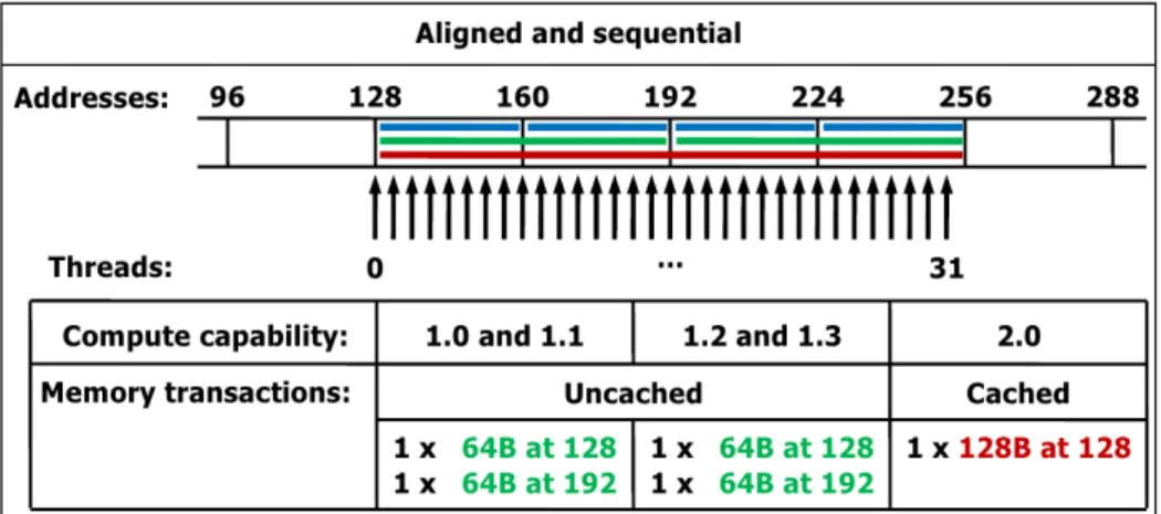
It is up to the programmer to choose the most appropriate location for the data, but it is even more important the way those data are accessed, especially when accessing the global memory: the controller is able to pack multiple requests to adjacent memory addresses into one long read, causing multiple potential memory access to collapse to a single one. Correctly aligned memory requests are referred to as coalesced. These pattern slightly change across different compute capabilities, but as a rule of thumb consecutive threads should access consecutive words in memory and memory requests should begin with addresses that are multiples of a word. Figures 3.4, 3.5 and 3.6 summarize, as showed in the CUDA Programming

Guide, how the hardware controllers of different compute capabilities are able to optimize non-consecutive or misaligned accesses, with important consequences on the overall performance.

One of the practices suggested by NVIDIA’s to improve coalesced accesses, for example, is to arrange the data in a structure of arrays fashion rather than an array

5

It is possible with some specific hardware configurations, e.g. integrated GPUs sharing RAM with the CPU.

3. CUDA 26

Figure 3.4: Coalescence - case 1: accesses are aligned and sequential (best case)

Figure 3.5: Coalescence - case 2: accesses are aligned but not sequential

3. CUDA 27

of structures [63]. Both MAGFLOW and GPUSPH are implemented following this

recommendation.

In some classes of problems, however, it is not possible to predict or correct the sparsity of some accesses. In the SPH model, for example, accessing the neighbors of consecutive particles often leads to misaligned memory accesses. We could think of putting in the list of neighbors a copy of the data instead of the addresses of the neighbor particles; however, this could require up to one hundred times more GPU memory and is thus unfeasible.

3.6

Contexts

A CUDA context is the set of variables and structures used internally by the CUDA runtime libraries to communicate with a specific device. The high-level API au-tomatically initializes a CUDA context when a CPU thread first tries to access a GPU, in a one-context-per-thread fashion; the low-level API instead allows to cre-ate multiple CUDA contexts and to switch from one to another within the same CPU thread. Using multiple GPUs with the high-level API requires therefore one CPU thread per device.

Since the recent release of CUDA 4.0, this is not necessary anymore, as it is possible to switch from one device to another within the same CPU thread with a specific high-level call [64]. As we implemented the simulator with CUDA 3.2

using the high-level API, we chose to launch one CPU thread per device. This also have the advantage of allowing a cleaner design and a more robust code, while transparently exploiting multiple CPU cores, if available, to perform the host tasks.

3. CUDA 28

3.7

Streams

A CUDA Stream is an abstraction for a logical sequence of operations that it is possible to run on the GPU. In a CUDA Stream it is possible to enqueue a kernel launch, a data transfer or a CUDA Event, a dummy structure needed for GPU timing and synchronization of streams. If multiple streams are run in parallel, and the pending operations of a stream are compatible with those of another stream (e.g. kernel and data transfer in older cards, two different kernels in devices with compute capability 2.0), the compatible operations are run simultaneously.

3.8

Asynchronous API

All kernel calls are non-blocking, i.e. the CPU code keeps executing after launching a kernel and CPU and GPU can work independently. To make the CPU code wait for a kernel to complete, for example when we need the result of the kernel computation, we can call the cudaThreadSynchronize() method. Memory transfers, instead, are by default blocking: a cudaMemcpy() method only returns when the transfer is complete. The CUDA platform offers the capability to run memory transfers concurrently with CPU and GPU computations. We access this functionality through the asynchronous API, which is a set of library calls mostly terminating with the -async suffix.

Listing 3.1 shows an example of concurrent kernels and memory transfers,

where the computations on the input data start as soon as the first part has been uploaded. Note that three different for cycles are used to iterate on a set of streams, enqueueing the operations in a breadth-first fashion. Although in some applications a depth-first fashion could be preferable (e.g. processing video streams), using distinct for cycles is necessary for actual asynchronous execution because of the way the CUDA library was designed. The CUDA runtime enqueues the operations in two internal queues, one for kernels and one for memory

trans-3. CUDA 29

fers. If all the operations of the same stream are enqueued in a row, the runtime scheduler will not find any compatible operation to the one being issued as they belong to the same stream. Listing3.2shows an “incorrect” depth-first enqueueing

leading to a synchronous execution.

1 / / e n q u e u e t h e u p l o a d o f p a r t s of t h e d a t a 2 f o r (i n t i = 0 ; i < N S T R E A M S; + +i) 3 c u d a M e m c p y A s y n c(i n p u t D e v P t r + i * p a r t i a l _ s i z e, 4 h o s t P t r + i * p a r t i a l _ s i z e, s i z e, 5 c u d a M e m c p y H o s t T o D e v i c e, s t r e a m[i] ) ; 6 / / e n q u e u e t h e p a r t i a l c o m p u t a t i o n s 7 f o r (i n t i = 0; i < N S T R E A M S; ++i) 8 M y K e r n e l< < <100 , 5 12 , 0 , s t r e a m[i] > > > 9 (o u t p u t D e v P t r + i * p a r t i a l _ s i z e, 10 i n p u t D e v P t r + i * p a r t i a l _ s i z e, s i z e) ; 11 // e n q u e u e t h e d o w n l o a d of t h e r e s u l t s 12 f o r (i n t i = 0; i < N S T R E A M S; ++i) 13 c u d a M e m c p y A s y n c(h o s t P t r + i * p a r t i a l _ s i z e, 14 o u t p u t D e v P t r + i * p a r t i a l _ s i z e, size, 15 c u d a M e m c p y D e v i c e T o H o s t, s t r e a m[i] ) ;

Listing 3.1: Example code for issuing concurrent kernels and memory transfers in a breadth-first fashion.

There are two requirements to use asynchronous transfers. The first is the usage of streams. A kernel and a memory transfer must be issued on different, non-zero streams. Issuing two operations on the same stream (or not specifying a stream, that results in using stream 0 for both) tells the GPU scheduler that the second depends on the first, and thus it has to wait for it to finish.

The second is that all CPU buffers involved in the transfers must be allocated as page-locked. When a CPU process is switched or paused by the scheduler, its memory area may be swapped in virtual memory by the operative system, and it is

3. CUDA 30

restored as soon as the process is active again. This may cause concurrency and/or inconsistency problems for asynchronous transfers, that remain alive despite the state of the issuing process. For this reason, we must ask the operative system to allocate a special kind of memory that is not paged (page-locked) even if the owner process is paused. CUDA offers some simplified methods to issue this special kind of allocation (cudaHostAlloc() or cudaMallocHost()). Page-locked memory is also faster than non page-locked, as it prevents page faults and enables direct GPU-RAM DMA transfers. However, it is advisable to minimize its use, as page-locking a large amount of RAM memory may result in increased swapping and reduced overall system performances.

1 // e n q u e u e t h e u p l o a d of p a r t s of t h e d a t a 2 f o r (i n t i = 0; i < N S T R E A M S; ++i) { 3 / / u p l o a d i n p u t d a t a 4 c u d a M e m c p y A s y n c(i n p u t D e v P t r + i * p a r t i a l _ s i z e, 5 h o s t P t r + i * p a r t i a l _ s i z e, siz e, 6 c u d a M e m c p y H o s t T o D e v i c e, s t r e a m[i] ) ; 7 / / k e r n e l l a u n c h 8 M y K e r n e l< < <100 , 5 12 , 0 , s t r e a m[i] > > > 9 (o u t p u t D e v P t r + i * p a r t i a l _ s i z e, 10 i n p u t D e v P t r + i * p a r t i a l _ s i z e, s i z e) ; 11 / / d o w n l o a d o u t p u t d a t a 12 c u d a M e m c p y A s y n c(h o s t P t r + i * p a r t i a l _ s i z e, 13 o u t p u t D e v P t r + i * p a r t i a l _ s i z e, size, 14 c u d a M e m c p y D e v i c e T o H o s t, s t r e a m[i] ) ; 15 }

Listing 3.2: Example code for issuing concurrent kernels and memory transfers in a depth-first fashion. Transfers are likely to be performed in a synchronous way.

3. CUDA 31

3.9

Libraries

Numerical problems often require high-level operations like sorting big arrays or finding the minimum/maximum element. As it is not trivial to implement such operations in an efficient way on parallel hardware, some pre-optimized libraries have been released to this aim.

For example, CUDPP (CUDA Data Parallel Primitives) is “a library of data-parallel algorithm primitives such as data-parallel prefix-sum (scan), data-parallel sort and paral-lel reduction” [65]. It runs on CUDA-enabled hardware and it is released under

the New BSD license 6

[77]. In particular, we use the CUDPP Radixsort [71] in

GPUSPH and the CUDPP minimum scan [72] in both MAGFLOW and GPUSPH.

Other libraries that are worth citing include CUFFT for parallel Fast Fourier Transform, CUBLAS for linear algebra solvers, CUSPARSE for efficient handling of sparse matrices, CURAND for quasi-random number generation and Thrust, a template library offering similar functions to CUDPP with a higher level of ab-straction.

6

The BSD license is a variant of GNU GPL allowing the code to be used in commercial, closed-source applications.

Chapter 4

Multi-GPU computing

We already mentioned that only problems exposing some degree of parallelism are suitable for a parallel implementation on the GPU. Numerical problems exposing a high level of intrinsic parallelism, however, can be mapped to more than one level of parallelism. In general, if a problem is modeled as a set of independent subproblems, then it is possible to split the set of required computations in two or more partitions that can be executed in parallel on separate devices.

4.1

Motivation

The main motivation to split a problem into multiple devices is the possibility to achieve a gain in performance. The highest theoretical speedup obtainable with D devices is D×, but in rare cases it can be even higher 1

.

For some problems there is also a memory reason. Some numerical problems can benefit from the increased total memory of a multi-device systems by working on a wider range of data or on inputs with higher density. It is the case of very wide or very dense SPH simulations, whose number of particles would not fit in the memory of one GPU.

1

For example, the split may relieve a congested PCI bus, increasing the data trasfer speed be-tween the CPU and the devices and therefore causing a superlinear speedup, as in [11].

4. Multi-GPU computing 33

In some cases, a substantial speedup or memory gain can even have conse-quences on the model level. With a problem that is solved one order of magnitude faster than the prospected time, for example, it is possible to think of applying a stochastic super-model to refine or bound the numerical results. A multi-device implementation of a numerical problem is more likely to reach such a result if it is robust and truly scalable, as it allows to increase performance proportionally to the available computing power.

However, while exploiting the computational power of a GPU is today far easier than at the beginning of the GPGPU era, porting a numerical solver to GPU in an efficient way is still far from trivial and exploiting more than one GPU at a time is even more difficult due to technical and model constraints. There exist multi-GPU softwares mainly for data compression and visualization [3, 45, 76], molecular

dynamics [82,52,67] and a few grid-based models [5, 68,83, 81, 66]. To the best of

our knowledge, however, no Navier-Stokes SPH simulator has been implemented for multi-GPU yet, although some works claim that a port to multi-GPU is in progress.

4.2

Naïve approach

A trivial approach to run a problem in parallel on multiple devices could be to split the problem domain, whatever it is, in a number of partitions equal to the number of devices to be exploited. Recalling that the graphic processor has its own, coupled memory, one could copy the necessary, partial data to the devices, perform the computations and finally transfer back the results; this should be repeated for every set of computations to be performed (e.g. every step of a simulation).

Given the bus data rate and the mathematical throughput of the computing units, it is easy to estimate the ratio between the two and the potential convenience of the approach. Unfortunately, except for very particular cases, the time required

4. Multi-GPU computing 34

to transfer the problem data largely overcomes the time required to perform the computations, making the whole process disadvantageous. Moreover, as direct device communication is in general expensive or even not possible, any inter-dependence among parts of the problems adds a technical constraint that must be carefully taken into consideration.

4.3

Subproblems inter-dependence

Some numerical problems, such as astrophysical n-body simulations, present com-pletely inter-dependent subproblems and therefore can not be easily split, as each element requires accessing sparse data of the whole domain. In these cases, one should rethink the model, if possible, or use an approximate solution. Some classes of problems expose instead a complete subproblem independence; in this cases, it is enough to partition the problem with a greedy strategy and run the subparts in parallel on different devices. We refer to these fully parallel problems as embarrass-ingly parallel.

Most problems are somewhere in the middle. The particle methods we will describe later, for example, are by definition made up of quasi-independent sub-problems: the state of a particle depends on the previous state of the same particle and on the state of neighbor particles only. It is possible to split such a problem as long as a proper overlap is left between the subproblems; we need to properly allocate, handle and keep updated this overlap.

4.4

Overhead

Running a problem on multiple devices introduces an unavoidable overhead due to the split operations and load balancing. Most problems, especially the ones involving some subproblem overlap, also require a variable amount of data to be

4. Multi-GPU computing 35

continuously transferred during the computations, to keep the overlaps updated and deal with dynamic changes (e.g. a particle “moving” from one device to an-other). Data transfers between a device and the host, as well as device-to-device transfers, are the predominant overhead factor in most multi-GPU implementa-tions. Moreover, as in the general case it is not possible to transfer data from one device to another in a direct manner, data must be first copied to the host and then copied back to the recipient device, thus doubling the already significant transfer times. Making all these overheads negligible is the main challenge of any multi-GPU system where a continuous inter-device communication is needed.

4.5

Speedup metrics

Comparing the performance of different problems is usually tricky and sometimes even unfeasible, due to the possible differences in the type of data or the measured parameters (e.g. speed vs. accuracy or input size). It is however possible to estimate the efficiency of a parallelization by means of measured speedup with respect to a single-core execution. We refer to cores for simplicity, but the following considerations are still valid for either multi-core, multi-GPU or generic many-core parallel computing.

A common starting point to analyze a parallel implementation is to model the problem as made by a parallelizable part and a serial, non parallelizable one. The latter includes operations which are performed anyway in a serial manner (e.g. file I/O) and operations that are introduced with the parallel implementation (overhead, e.g. load balancing). Let α be the parallelizable fraction of the problem and β the non parallelizable one; it is α+β =1, with α, β non-negative real

num-bers. For embarrassingly parallel problems α is equal or very close to 1; problems intrinsically serial, where each step depends on the outcome of the previous one, have β ≈ 1. It is advisable, when the model allows for it, to formulate a problem

4. Multi-GPU computing 36

in a way to minimize β to the strictly necessary.

4.5.1

Amdahl’s law

Amdahl’s law, introduced in 1976 by the computer architect Gene Amdahl [2],

measures the speedup in terms of execution time and gives an upper-bound in-versely proportional to β. Although it is mainly used in parallel programming, where number of available computing units is often directly related with the ob-tainable speedup, it can be used in the analysis of a serial problem when only a portion of it is being improved.

With a slight change in the notation, Amdahl’s law can be written as

SA(N) =

1

β+ α

N

(4.1)

where N is the number of used cores and SA the theoretical maximum speed-up.

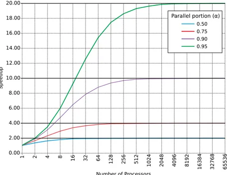
Fig.4.1plots the outcome of the law with different ratios α/β, the asymptotic limit

of each being 1/β. 20.00 18.00 16.00 14.00 12.00 10.00 8.00 6.00 4.00 2.00 0.00 S p eed u p 1 2 4 8 _{16 32 64} 128 256 512 _{1024 2048 4096 8192} 16 3 8 4 32 7 6 8 65 5 3 6 Number of Processors Parallel portion (α) 0.50 0.75 0.90 0.95

4. Multi-GPU computing 37

Amdahl’s law assumes that the problem size is fixed and the number of cores is the only variable. The intuitive meaning is rather simple: the time Tp required

to solve a problem with N cores is Tp = βT1+αT1/N, and the ratio T1/Tp

(equiv-alently, 1/Tp with T1 =1) is the expected speedup.

In case the parallel fraction is not known a priori, it is possible to rewrite the formula for α: αestimated = 1 Se −1 1 N −1 (4.2) where Se is the empirical speedup obtained with N cores.

4.5.2

Gustafson’s law

In 1988 J. Gustafson et. al. proposed a different speedup model [29], claiming that

Amdahl’s law was way too restrictive. In particular, they challenged the assump-tion that the problem size is always fixed, remarking that the size of a problem often scales with the available raw computing power. In other words, as they clearly explain in the paper, “rather than ask how fast a given serial program would run on a parallel processor, we ask how long a given parallel program would have taken to run on a serial processor”.

Gustafson’s law can be formulated as:

SG(N) = N−β· (N−1) (4.3)

The obtained speedup is equal to the number of used cores minus the non paral-lelizable fraction, that makes N−1 cores unexploited for β fraction of the problem. The plot of Gustafson’s law is just a line less steep than x = y. With this formu-lation, there is no theoretical upper-bound to the speedup, as long as it is always possible to indefinitely increase the workload. When compared to Amdahl’s law, this is often referred to as scaled speedup.

4. Multi-GPU computing 38

4.5.3

Karp–Flatt metric

The Karp–Flatt metric was proposed in 1990 as a measure of the efficiency of the parallel implementation of a problem [47]. The new efficiency metric is the

experimental measure of the serial fraction β of a problem. As it can be imagined, this can be proven to be consistent with Amdahl’s approach, and can be derived from it.

With another slight notation change, it is:

βKF = 1 Se − 1 N 1− 1 N (4.4)

where Se is the empirically measured speedup and N is the number of cores, as

usual. This can also be obtained from Amdahl’s law by rewriting for β. Since this a posteriori metric measures both serial time and introduced overhead, it is especially useful to apply to at least two executions with different N: a constant

βKF means the the parallelization was efficient, while a growing βKF means that

some overhead is being introduced by the growing number of cores.

4.6

Linear overhead

We already mentioned that the highest theoretical speedup obtainable with D de-vices is D× and that, except for the so called embarrassingly parallel problems, we usually introduce some overhead due to the synchronization and data transfer operations. We now informally analyze the consequences of a linear cost (i.e. βKF

linear with the number of devices), which occurs when a non perfect paralleliza-tion is implemented or no dynamic load balancing is used.

We may wonder, for a specific problem, at what point the introduced overhead exceeds the advantage of increasing the number of devices by one, thus determin-ing an upper-bound to the number of devices that is convenient to use. Please

4. Multi-GPU computing 39

note that in this context we use the word convenient referring to the performance metrics (using D devices is convenient if the problem is solved faster than using D−1 devices), and not to the memory gain.

Let us compute first the performance gain of using D devices instead on D−1, in an ideal case. Say T the time required to solve a problem with one device. It will take T/D time to solve the problem with D devices, and T/(D−1) with D−1 devices. Using D devices takes

T D−1− T D = T( 1 D−1 − 1 D) = T D(D−1)

time less than using D−1 devices. Dividing by T we obtain the gain in percent: 1

D(D−1) (4.5)

This number decreases quite fast. Table4.1shows the progressive gain, in percent,

from 2 to 8 devices. For example, using 8 devices we expect a problem to be solved in 1/(8(8−1)) ≈ 1, 8% less time than using 7 devices.

Let Q be the overhead introduced each time we increase by one the number of used devices; it is possible to estimate the mentioned upper-bound Dmax by

choosing the maximum D for which the inequality

Q/T< 1

D(D−1) ⇒

Q< T

D(D−1) (4.6)

holds. It is implicit that for the inequality to be defined it must be D> 1 (indeed, we can safely assume that it is convenient to use one device instead of zero) and T >0 (no need to split a simulation that takes no time).

4. Multi-GPU computing 40

Devices 2 3 4 5 6 7 8

Progressive gain 50, 00% 16, 7% 8, 3% 5% 3, 3% 2, 4% 1, 8%

Table 4.1: Ideal progressive gain, in percent, when using 2 to 8 devices

4.7

Timeline profiling

While debugging and testing our first multi-GPU prototypes, we soon felt the need to profile accurately the execution of the simulations across multiple devices to find out the effectiveness of asynchronous operations and to detect potential bugs and unwanted race conditions.

In year 2008 NVIDIA released the Visual Profiler, a multi-platform profiling utility now provided as part of the CUDA SDK tools [16]. The Visual Profiler runs

a CUDA program in a special environment that makes the CUDA runtime log information about the ongoing operations. Example of information include the number of cache hits and misses, timestamps and duration of kernel executions and memory transfers, number of coalesced and uncoalesced memory access, occu-pancy of a kernel, and other. Is is also possible to add custom fields by using special registers within the kernel code. However, the Visual Profiler did not provide until recently a graphical plot and comparison of the execution timelines, especially for multi-GPU environments. Moreover, all asynchronous operations were made syn-chronous for logging purposes, voiding any possibility to check the actual overlap between transfers and computations.

The CUDA runtime offers the possibility to log, optionally in CSV format, in-formation such as the beginning and ending timestamps of any kernel or transfer performed on the GPU, as long as some special environment variables are set. It is not easy to interpret the logged information, as this feature is very poorly documented and the meaning of some fields is still unknown, but this allows not to lose the overlap among asynchronous operations. We then implemented a little tool that takes in input the log of an execution and produces a custom multi-device

4. Multi-GPU computing 41

timeline in SVG format.

The output is a fully configurable timeline with indications about the absolute and relative execution times. It shows the time at which an operation has been issued on the CPU and the time it was actually performed on the device. Thanks to the powerful ECMA script feature of the SVG standard, it is possible to see detailed informations about an event just by hovering the mouse on an event, as shown in fig. 4.2. It is possible to configure via command-line a number of

graphical parameters (e.g. horizontal drawing scale) and filtering options (e.g. hide CUDPP calls or replace decorated kernel names); the visualization can be organized by method name (fig. 4.2) or by stream (fig. 4.3) and it is possible to

show the timelines of different GPUs in the same view. The only important limit currently known is the lack of an accurate synchronization between timelines of different devices. Unfortunately, each device uses its own clock-driven timeline and there is no documented way to fix an absolute relation between any two. We thus had to synchronize by means of different estimates, e.g. knowing the process start time or timing a dummy kernel launch as a reference.

Figure 4.2: Timeline produced for a 3-GPUs MAGFLOW simulation (only 2 are shown). The overlap between the bordering slice transfer (in purple) and the CalcFlux kernel (in read) is immediately recognizable. Together with the yellow popup, two event delimiters appear on hovering, to compare the event time with other events even in different GPUs.

4. Multi-GPU computing 42

This little tool boosted the testing and debugging process of both simulators, al-lowing to rapidly find minor bugs that prevented some operations or even different devices to overlap their execution. In general, a detailed graphical representation of what is really happening in the device helps to evaluate quickly the efficiency of new design hypotheses and fine tune execution parameters.

Stream 0 Stream 1 Stream 2 Stream 3 431.755ms 531.755ms Stream 0 Stream 1 Stream 2 Stream 3 431.755ms 531.755ms Stream 0 Stream 1 Stream 2 Stream 3 431.755ms 531.755ms

stream: 0; dir.: -; size: 0; mem_type - method: buildNeibs; on gpu: 16132.4µs; row: 125;

Figure 4.3: Timeline produced for a 3-GPUs GPUSPH simulation, aligned by stream. Note the dependency of memory transfers on previous kernels of the same stream, esp. in GPU n.3 (the central one of the simulation, with 2 bordering slices).

The timeline feature, which at the time we started working on multi-GPU was only available as a plugin for the Microsoft Visual Studio commercial IDE for Windows [15], seems to have been finally introduced in recent CUDA 4.1RC release

[14]. Although one of the counters is supposed to measure the overlapping ratio

of calls to the asynchronous API, it seems many calls are still made synchronous, and this is confirmed by the bad performance of programs being profiled. It is therefore still not possible to profile a multi-GPU program and track the actual amount of asynchronous operations unless using a non-official profiler like the one we developed.

In the future, the timeline tool might be improved for general use with a user friendly interface and, most important, an automatic system to synchronize the

4. Multi-GPU computing 43

timelines of different devices (e.g. with a timed dummy kernel launch).

4.8

Testbed

4.8.1

MAGFLOW

Our test-bed for the MAGFLOW simulator was the simulation of the lava erup-tion on Etna volcano in the year 2001 on DEMs with 2m and 5m resoluerup-tion. In this scenario there is a single vent emitting up to 30m3/s fluid lava with a pseudo-gaussian trend. The lava was modeled with a Bingham rheology [9] and

a Giordano-Dingwell viscosity [24] with a solidification temperature of 800◦ and a

0.2% water percentage. Some sets of simulations were resumed from one already 19% complete, where the bounding box of the active flow had already reached its maximum extent.

4.8.2

GPUSPH

In GPUSPH the scenario to be simulated (topology plus various parameters) is en-capsulated into the C++ virtual class Problem. A class that inherits from Prob-lem must define the environment (e.g. walls) and the amount and initial shape of fluid. Optionally, it is possible to override the default physical and simulation parameters. We used two classes in particular, DamBreak3D and BoreInABox, both defining a 0.43m3 parallelepiped of water in a box. The former containes a column-shaped obstacle almost in the center; the latter has a wall on one side par-tially containing the fluid and an optional second wall making a corridor. In the DamBreak3Dthe fluid flows almost evenly in the domain, while in BoreInABox the flow soon becomes strongly asymmetric and flattens afterward in the non-corridor variant. The SPH is set to use a Wendland kernel with a density in the range 4·10−3...4·10−3; the fluid was modeled with an artificial viscosity law

4. Multi-GPU computing 44

(α=4) and a speed of sound c=300·0.4·g m/s.

4.8.3

Hardware

Our testing platform is a TYAN-FT72 rack mounting 6×GTX480 cards on as many 2nd generation PCI-Express slots. The system is based on a dual-Xeon processor with 16 total cores (E5520 at 2.27GHz, 8Mb cache) and 16Gb RAM in dual channel. Each GTX480 has 480 CUDA cores grouped in 15 multiprocessors, 48Kb shared memory per MP, 1.5Gb global memory with a measured datarate of about 3.5Gb/s host-to-device and 2.5 Gb/s device-to-host (with 5.7 Gb/s HtD and 3.1 Gb/s DtH peak speeds for pinned buffers).

The operative system is Ubuntu 10.04.2 LTS Lucid Lynx 2.6.32-33-server SMP x86_64, gcc 4.4.3, CUDA runtime 3.2 and NVIDIA video driver 285.05.09.

Part II

Chapter 5

The MAGFLOW simulator

The MAGFLOW model is an advanced state-of-the-art Cellular Automaton (CA) for lava flow simulation. Its physics-based cell evolution equation guarantees ac-curacy and adherence to reality, at the cost of a significant computational time for long-running simulations. We here provide an overview of the related work, then describe the model behind the simulator and finally the single- and multi-GPU implementations.

5.1

Related work

The CA-based approach is probably one of the most successful for the simulation of a lava flows [17, 43, 54, 4]. The computational domain is represented by a

regular grid of 2D or 3D cells, each characterized by properties such as lava height and temperature; an evolution function for the properties of the cells models the behavior of the fluid.

The MAGFLOW model [80] is a cellular automaton developed at INGV-Catania

and capable of modeling many physical phenomena of lava flows like thermal effects and temperature-dependent viscosity change.

(vali-5. The MAGFLOW simulator 47

dation) and to predict the behavior of the lava flow in real-time during the Etna eruptions of 2004 [20], 2006 [37,79] and 2008 [10]. It has been possible to use it for

forecasting purposes thanks to its fast GPU implementation, which can simulate several days of eruption in a few hours.

5.2

Model

We here describe briefly the MAGFLOW model as necessary basis to understand the single- and multi-GPU implementation; for a detailed description please refer to [80].

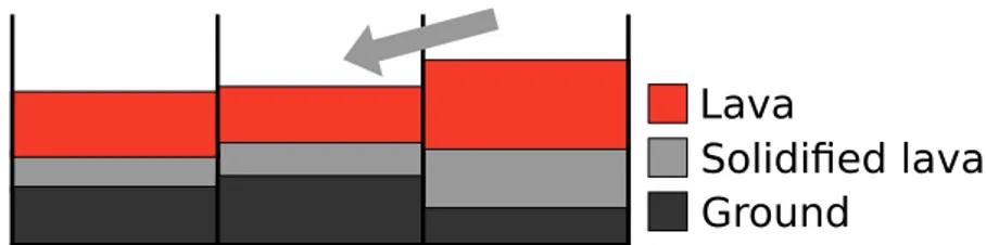
The simulation domain is modeled as a regular 2D grid of cells whose side matches the resolution of the DEM (Digital Elevation Model) available for the area. Each cell carries five scalar properties: ground elevation, fluid lava thickness, so-lidified lava thickness, heat and temperature. Cells marked as “vent” also have a lava emission rate, which is usually time-dependent.

The state of a cell at step s depends on the state of the eight neighboring cells (Moore neighborhood) and on the state of the same cell at step s−1. The lava flux between each pair of neighboring cells is determined according to the height differ-ence using a steady-state solution for the one-dimensional Navier-Stokes equations for a fluid with Bingham rheology.

Ground

Solidified lava Lava

Figure 5.1: Section of three adjacent cells with ground elevation, solidified lava and fluid lava.

The total flux of each cell depends on the lava emission (for vent cells) plus any lava flux with neighboring cells. The actual lava variation is given by the total flux

5. The MAGFLOW simulator 48

Q multiplied by the timestep δt for that iteration. A numerical constraint upper-bounds δt to prevent nonphysical simulations. Each cell computes its maximum and the minimum of the maxima is chosen as global timestep.

Each iteration of simulation consists of the following steps: 1. Compute the lava emitted by active vents;

2. Compute the cross-cell lava flux between each pair of neighbors; 3. Find the minimum timestep among the computed maxima;

4. Integrate the flux rate over the chosen timestep: compute new lava thickness, solidified lava and heat loss.

The MAGFLOW simulator was initially developed only for serial CPU exe-cution. As the model suits well a parallel implementation, it was ported to be executed on a many-core GPU.

5.3

Single-GPU MAGFLOW

Porting MAGFLOW to CUDA was relatively easy due to the implicit parallel na-ture of the model. Each cell only depends on the previous state of the same cell and of a small number of neighbors (eight); the only global operation is finding the minimum δt. We can therefore run one thread per cell and let them run in parallel, each computing its next state.

The CPU implementation of MAGFLOW defined a Cell structure holding the data for each cell; the automaton was essentially a list of Cells. The GPU version of MAGFLOW defines instead an array for each property of the cells. This follows the NVIDIA recommendation to use structures of arrays rather than arrays of structures [63], and it is aimed to improve coalescence in memory accesses.

The four steps of the CPU implementation were straightforwardly implemented as GPU kernels:

5. The MAGFLOW simulator 49

1. Erupt: for each cell, compute lava emission if it is a vent (parallel);

2. CalcFlux: for each cell, compute the final flux by iterating on neighbors, sum the partial fluxes and compute the maximum δt (parallel);

3. MinimumScan: find the minimum δt (global scan);

4. Update: compute new lava thickness, solidified lava and heat loss (parallel). As showed in the list, the only operation that is not truly parallel is the mini-mum scan, for which the CUDPP library is used.

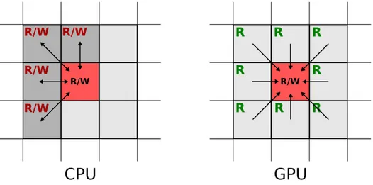
The main difference between the serial CPU-based implementation and the par-allel GPU-based one is the number of times interactions are computed. The CPU code computes the interaction between two cells once and adds the contribution to both cell (with proper change in sign). The GPU benefits instead from totally independent and parallel computations, and it is more efficient to let each cell compute the interactions with all its neighbors, even if this means computing each interaction twice. This approach simplifies the implementation substantially, since it avoids the concurrency problems that have to be dealt with when partial results are stored on cell by multiple neighbors.

R

CPU

GPU

Figure 5.2: The CPU code computes the interaction of a pair of neighbors once and adds the partial on both; the GPU code computes all the interactions for each cell and only writes self total.

5. The MAGFLOW simulator 50

As mentioned in section2.3, numerical results may vary a little with respect to

the CPU implementation as partial fluxes are added together in a different order. We use the Kahan summation algorithm to mitigate this difference. Moreover, the CPU implementation used double precision while most GPU simulations are run on cards featuring hardware single precision. The numerical differences, however, do not alter the simulation significantly.

The performance results of the GPU implementation are quite impressive. The speedup factor depends on the hardware used, the topology of the flow and the DEM resolution. For example, the higher the DEM resolution, the more saturated is the GPU, thus better covering all transfers and other GPU-related overheads. In the general case, it is safe to say that on recent hardware (i.e. GTX480) the speedup over the reference serial implementation for single-core CPUs varies from 50×to 100×, taking only tens of seconds to simulate a one week eruption.

More details on the implementation, validation and performance gain of the GPU-based MAGFLOW can be found in [8].

Chapter 6

Multi-GPU MAGFLOW

We here describe how the parallel, GPU-based MAGFLOW was adapted to run on multiple GPUs simultaneously, thus exploiting a second level of parallelism.

6.1

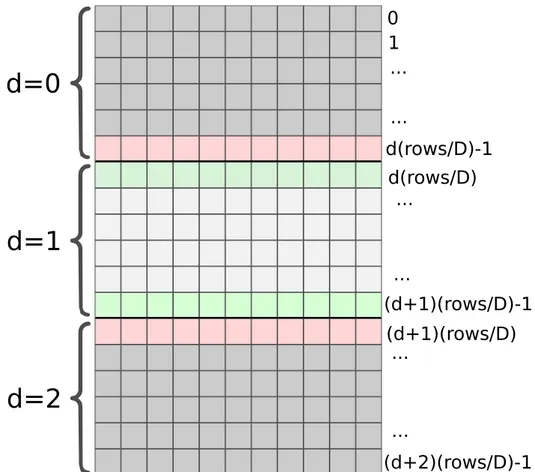
Splitting the problem

There are in general at least two ways to exploit a second level of parallelism for an already parallel problem: splitting the set of data to be elaborated (space domain) or split the set of computations to be performed (computational domain).

The simplest and most intuitive is to split the automaton domain into separate areas and assign each area to a different device. Because the flux computation for every cell requires to access its immediate neighbors, the split areas need to have some degree of overlap.

We could instead divide the problem in the domain of computations, assigning each phase of the computation to a different device (in pipeline). This approach presents unfortunately three major drawbacks: it is not possible to scale to an arbi-trary number of devices; it is not trivial to balance computational load among the devices; it requires the complete domain to be continuously transferred through all active devices during the whole simulation. For these reasons, we chose the