UNIVERSITÀ DELLA CALABRIA
Dipartimento di Ingegneria Informatica, Modellistica, Elettronica e Sistemistica
Scuola di Dottorato
Scienza e Tecnica “Bernardino Telesio” XXVIII CICLO
Con il contributo della Regione Calabria POR Calabria FSE 2007/2013 – Asse IV Capitale Umano
Obiettivo Operativo M.2
SURVEY, DIAGNOSIS AND MONITORING OF STRUCTURES
AND LAND USING GEOMATICS TECHNIQUES:
THEORETICAL AND EXPERIMENTAL ASPECTS
Settore Scientifico Disciplinare ICAR/06
Direttore: Ch.mo Prof. Roberto Bartolino
Supervisore: Ch.mo Prof. Raffaele Zinno
Dottorando: Dott.ssa Serena Artese \
SURVEY, DIAGNOSIS AND
MONITORING OF STRUCTURES
AND LAND USING GEOMATICS
TECHNIQUES: THEORETICAL AND
EXPERIMENTAL ASPECTS
RILIEVO, DIAGNOSI E
MONITORAGGIO DI STRUTTURE E
DEL TERRITORIO CON TECNICHE
GEOMATICHE: ASPETTI TEORICI
E SPERIMENTALI
La presente tesi è cofinanziata con il sostegno della Commissione Europea, Fondo Sociale Europeo e della Regione Calabria. L’autore è il solo responsabile di questa tesi e la Commissione Europea e la Regione Calabria declinano ogni responsabilità sull’uso che potrà essere fatto delle informazioni in essa contenute.
Abstract
The Geomatics techniques for the detection and representation of the land and objects have seen an exceptional development in recent years. The applications are innumerable and range from land planning to geophysics, from mitigation of landslide risk to monitoring of artifacts, from cultural heritage to medicine.
With particular regard to the structures and to the land, the technologies used can be divided into three categories: techniques based on the acquisition and processing of images, techniques based on the measurement of angles and distances, and combinations of the foregoing.
After an overview of Geomatics techniques and their basic theoretical concepts, a number of aspects have been thoroughly investigated. There follows a series of applications of the techniques described. Finally two new applications for deflection measurement of bridges under dynamic load are presented.
Riassunto
Le tecniche geomatiche per il rilievo e la rappresentazione del territorio e degli oggetti hanno avuto negli ultimi anni uno sviluppo eccezionale. Le applicazioni sono innumerevoli e spaziano dalla pianificazione del territorio alla geofisica, dalla mitigazione del rischio idrogeologico al monitoraggio di manufatti, dai beni culturali alla medicina.
Con particolare riguardo alle strutture e al territorio le tecnologie utilizzate possono essere distinte in tre categorie: tecniche basate sull’acquisizione ed il trattamento di immagini, tecniche basate sulla misura di angoli e distanze, combinazioni delle precedenti tecniche.
Dopo una panoramica delle tecniche geomatiche e dei rispettivi concetti teorici di base, alcuni aspetti sono approfonditi. Seguono una serie di applicazioni delle tecniche descritte. Infine vengono presentate due nuove applicazioni per la misura della deformazione di ponti sottoposti a carico dinamico.
Contents
Introduction ……… 1
1. Geomatics techniques and tools for survey ……… 4
1.1 Total Station ……… 10
1.2 GNSS ……… 15
1.3 Laser Scanning ……… 31
1.3.1 Full Waveform processing laser scanner… 65 1.4 Photogrammetry ……… 69
1.4.1 Digital Image Correlation (DIC)……… 83
2. The surveying of Cavalcanti palace ……… 88
3. Integration of 3D surveying techniques: the case of the Escuelas Pias Church in Valencia ……… 94
4. The investigations carried out on the church of S. Maria dei Longobardi in S.Marco Argentano ……… 120
5. The survey, representation and structural modeling of ancient and modern bridges ……… 126
6. The DIC method used for the test of some composite material specimens ……… 148
7. Landslide monitoring ……… 166 8. Dynamic measurements: the use of a laser pointer for monitoring bridge deflections ……… 182
9. Dinamic measurements: the use of TLS and GNSS for monitoring the elastic line of a bridge ……… 192
10. Conclusions and ideas for future developments.. 203 11. References ……… 208
1
Introduction
The continuing evolution of surveying techniques and 3D modeling, and, more generally, of Geomatic techniques based on sensors and the development of ever more efficient systems for the display of digital data, highlights the added value of the use of these methods in the field of evaluation, diagnosis and monitoring of structures and land.
In particular, there is a growing awareness about the active contribution that these technologies can provide in interpretation, storage, and data archiving and enhancement of detected objects.
The growing role of survey methods and digital three-dimensional modeling, in structural and territorial fields, is confirmed by the growth in demand, and their increasing use at different levels of scale and
2
resolution. Obviously the use of these instruments fits within the coding of a cognitive process, in which particular attention is paid to the integration of both traditional and innovative methods.
Some theoretical and experimental aspects related to surveying, diagnosis and monitoring of structures and land using geomatics techniques are described in this dissertation. Its structure and brief explanations of the chapters are presented as follows:
Chapter 1 explains the Geomatics techniques and the operating principles and the most common uses of the instruments for 3D data capture in the structural, cultural heritage and territorial fields.
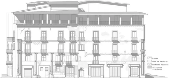
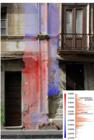
Chapter 2 describes the case study of the Cavalcanti Palace. In order to evaluate the vulnerability of the building surveys on the building were carried out to define the state of degradation and the crack pattern. A special survey was carried out to check the verticality of the main facade using the total station.
Chapter 3 describes the survey of the Escuelas Pias Church in Valencia. The creation of the 3D model and results of some investigations has allowed the formulation of a hypothesis about the design of dome.
3
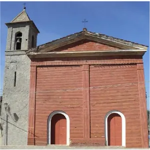
Chapter 4 describes the investigations carried out on the church of Santa Maria dei Longobardi, in San Marco Argentano, to understanding the structure of the facade.
Chapter 5 describes the activities, instruments and techniques used for surveying and modeling operations, along with the deviations between models and "as built", of ancient and modern bridges.
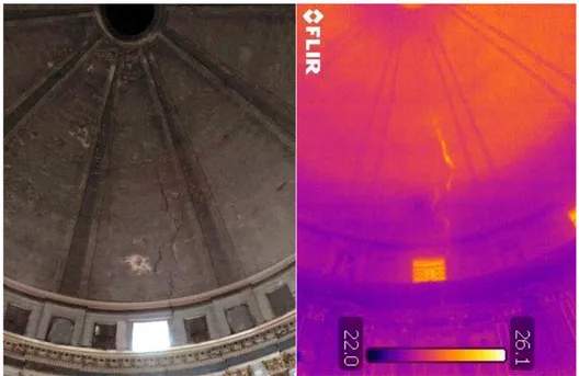
Chapter 6 describes the experiments conducted using the DIC method for the testing of some composite material specimens; the test has been integrated with an IR survey.
Chapter 7 describes the operations regarding the surveys of two landslides useful for evaluating dynamic and evolutionary mechanisms present in these areas and to predict possible scenarios of transformation.
Chapter 8 describes a new procedure to measure the dynamic deformation of a structure using a laser pointer.
Chapter 9 describes a new procedure to measure the dynamic deformation of a structure using laser scanner.
Chapter 10 presents the conclusions of this dissertation and recommendations for future research work.
4
1
Geomatics: techniques and
tools for survey
Geomatics is a field of activity which,using a systematic approach, integrates all the means used to acquire and manage spatial data required as part of scientific, administrative, legal and technical operations involved in the process of production and management of spatial information. These activities include, but are not limited to, cartography, control surveying, digital mapping, geodesy, geographic information systems, hydrography, land information management, land surveying, mining surveying, photogrammetry and remote sensing.
Definition by the Canadian Institute of Geomatics in their quarterly journal "Geomatica"
5
Geomatics comes from the French word gèomatique. It comes from the greek geo (earth) and informatics (information + automation + ics) [Kemp, 2008].
The first use of this term is documented in the early 1970s, in France, when the Ministry of Equipment and Housing established the Commission permanente de la géomatique. After that this term was no longer used for several years.
In 1981, the term was reinvented by Michel Paradis, a French-speaking surveyor. He was a photogrammetrist working for the Ministry of Natural Resources in the Quebec Provincial Government, and used this term for a keynote paper he wrote for the 100th anniversary symposium of the Canadian Institute of Surveyng (which became the Canadian Institute of Geomatics)[Paradis, 1981].
With this term, he underlined the common aspects among the disciplines involved in data acquisition, processing, and dissemination of spatial data (surveying, photogrammetry, geodesy, hydrography, remote sensing, cartography, and GIS). In 1986, the Department of Surveyng at Laval University, driven by Pierre Gagnon, introduced the first academic program on geomatics in the world, thus replacing its surveying program [Bédard et al. 1987]. In 1989, the University changed the name of the Department (Geomatics Sciences), of the Faculty (Forestry and Geomatics) and
6 created the Centre for Geomatics.
Surveying departments at the University of Calgary and the University of New Brunswick also adopted this new name between the late 1980s and early 1990s, when they changed their identification as well as the titles of their degrees.
The term “geomatics” is nowadays widely used all around the world. It is commonly recognized that Canada is its motherland.
Geomatics includes the instruments and techniques used in land surveying, remote sensing, cartography, GIS (geographic information systems), GNSS (Global Navigation Satellite System), photogrammetry, geophysics, geography and mapping.
In a wider interpretation, Geomatics includes all techniques related to spatially referenced information. There are many disciplines and techniques that constitute geomatics [Gomarasca, 2009]:
Computer science: considered as a science of representation and the processing of applicable information through the development of technological tools (hardware) and of methods, models, algorithms and systems (software).
Geodesy: the science that studies the shape and size of the Earth to define the reference surface in its complete form, the geoid, and in its simplified form, ellipsoid, and its external
7
gravitational field as a function of time.
Topography: started with and as part of geodesy. It is the set of procedures of direct land surveying. Topography is a combination of methods and instruments to measure and represent the details of the Earth's surface by planimetry, altimetry, tachymetry and land surveying.
Cartography: the description of the shape and dimension of the Earth and its natural and artificial details, by means of graphical or numerical representation of more or less wide areas, following fixed rules.
Photogrammetry: the science that determines the position and shapes of objects by measuring them from photographic images.
Remote sensing: the remote capture of data relating to territorial and environmental data, and the set of methods and techniques for their subsequent processing and interpretation.
Global Positioning System (GPS): this is used to determine the three-dimensional (3D) position of fixed or moving objects, in space and time, all over the Earth’s surface, under any meteorological conditions and in real time.
Laser scanning: this is used for the identification of subjects and the measurement of their shape and dimensions by means of the incident radiation in
8
the optical frequencies (0.3–15 μm) of the electromagnetic spectrum.
Geographical Information System (GIS): a powerful combination of instruments capable of receiving, recording, recalling, transforming, representing and processing georeferenced spatial data.
Decision Support Systems (DSS): These are associated with and made up of sophisticated information systems, able to create a number of evolutionary scenarios by modeling of reality and then to provide the decision maker’s choice from various possible solutions.
Expert System (ES): these are tools that can mimic cognitive processes made by the experts and their ability to manage the complexity of a real situation by means of interdependent processes of abstraction, generalization and approximation.
WebGIS: these are networked systems for the dissemination of geographic data stored on machines dedicated to the storage of databases, according to a complex network architecture.
Ontology: this is simplified view of the world that consists of a set of types, properties, and relationship types.
The Geomatics techniques use sensors. In particular, the three-dimensional sensors are tools to generate a
9
3D model of the scene they are surveying [Russo et al., 2011]. Of particular importance are the sensors based on the use of light radiation, within which a further distinction can be made according to the nature of the light used to perform the measurement. Methods using natural light are called "passive" (photogrammetric technique, theodolites, etc.); but if the light is encoded so as to play a role in the measurement process, they are called "active sensors" (laser scanners, structured light projection instruments, radar, total stations, etc.).
Active optical sensors [Blais, 2004; Guidi et al. 2010] map directly to the spatial position of the surface or the point detected, sometimes coupled to information color. This type of active instruments has the main advantage of acquiring directly and in a short space of time large amounts of data relating to a very complex geometry with an accuracy boost. The combination of these features makes this kind of instrument ideal for many applications, both at long and close range, but not suitable for all environmental conditions and the material characteristics of the artifacts [El-Hakim et al., 1995].
10
1.1 Total Station
The first instrument for the measuring of angles was the optical transit. In the 1970's, the electronic theodolite began to replace the optical transit because it measured angles more accurately. By the early 1980’s there appeared a new instrument called “total station" an electronic/optical device that was able to perform all necessary measurements (total) by using different techniques in one single device (station). It is, therefore, an electronic theodolite (transit) to read angles integrated with an Electronic Distance Meter (EDM) to read slope and distances, allowing storage of the measurements performed, without having to transcribe these accounts manually.
The basic components of a total station are [Ghilani and Wolf, 2011]:
The alidade: the upper mobile part of instrumentation that includes, the telescope and EDM, the angle meausurment system, the vertical circle, the microprocessor, the keyboard and the display, and the communication port. It is a shell, made of light aluminum alloy. Inside, on the
11
uprights and at the bottom, are allocated the circles to the angular readings, the various sensors and electronic devices, with the relative cabling, necessary to the overall management of the station, and also, in the robot stations, small electric motors implementing controlled rotations of the alidade and telescope. In the lower part, there are also provided one or two openings, diametrically opposite, used for mounting the panel reserved for the keyboard and the display.
The telescope is short, has reticles with crosshairs etched on glass, and is equipped with rifle sights or collimators for rough pointing (recent models are equipped with laser pointers). The telescopes, generally, have two focusing controls. The first, the objective control, is used to focus on the object being viewed; the second, the eyepiece, is used to focus on the reticle. The EDM, electronic distance meter, is assembled so that its axis coincides with the line of sight of the telescope, so the telescope and the EDM are coaxial. The distance measurement can be carried out with the reflector prism (range of some kilometers), or reflectorless in which the reflection takes place directly on the collimated object (range of two kilometers). The EDM uses electromagnetic (EM) energy to determine the length
12
of a line. The light radiation emitted by EDM to the prism reflectors, or to the surfaces of objects in the non-prism mode, comes from that reflected by the prisms and redirected to the device, which is detected by a photosensitive sensor. The radiation, then, is converted into electrical signals that allow the measurement of distance by means of the technique of phase measurement, that is, evaluated in the phase difference between the beam sent and the return, or the technique of measuring pulses, in which the flight time of a light pulse returning to the device is rated.
The base: this is a static part of instrument which has three pivots inserted in three corresponding holes of the tribrach, and here retained by the security device.
The tribrach: consists of an upper plate having three holes where the three correspondents pivots of the base are insert, a clamping device to secure the base of the total station or accessories, and a circular level (bull's-eye bubble); three screws for leveling; a lower plate with thread to attach the tribrach to the head of a tripod.
The optical plummet and laser plummet: built into tribrach or alidade and permits accurate centering over a point. In newer instruments, laser plummets have replaced the optical plummet.
13
Three classes of total station are available: Manual, semiautomatic and automatic [Gopi, 2007]. With the manual station, it is necessary to read the horizontal and verticals angles manually. The Semiautomatic Stations have mechanical motors allowing motorised angle movements both on the vertical and horizontal axes. When a servo station is able to recognise and track a reflector prism, it is called an Automatic Station. This characteristc is called Autolock by Trimble and Automatic Target Recognition (ATR) by Leica. The position of target is recognised from the station using either radio waves or imaging technologies. When the station can be controlled from a distance via remote control it is known as a Robotic total station. In the late 1990s, the swedish Dandryd introduced the first robotic total station called the Geodimeter.
The very latest total stations offer several functionalities that benefit standard surveying, like the systematic survey of the control points located on a monitored structure, grid scanning and atmospheric correction. With the grid scanning function the surveyor can programme the station to measure points by specifying a view window area and setting the horizontal and vertical intervals of the points to be measured. Rather than needing to aim at each individual
14
point, it is only necessary to decide the optimum point interval, the grid interval, in order to represent the object with sufficient accuracy. The distance measurement is based on the evaluation of a light signal that penetrates the atmosphere, which depending on the variability of its condition, influences the precision of measurement. The latest total stations, once inserted weather conditions, automatically apply to crude measure carried out a due correction.
The maximum accuracy of Total Stations is 1 mm/km for the distance and 0.5” for the angles.
In recent years, total stations coupled to an antenna system were produced with a GPS receiver mounted statically on the same station, or traveling on a telescopic pole. This allows us to integrate satellite measurements with those made by the station, determining the position of the instrument or points detected.
Total Stations are used today in many fields of application: engineering, topography, geology, architecture, Industrial modeling, Marine, Archaeology and Cultural Heritage, monitoring. In recent years they have been used to measure the movement of structures and natural processes with good results [Hill and Sippel 2002; Kuhlmann and Glaser 2002; Cosser et al., 2003; Gairns, 2008].
15
1.2 Global Navigation Satellite
System (GNSS)
The Global Satellite Navigation Systems (GNSS) are systems for geo-radiolocation and terrestrial, maritime or air navigation, based on a constellation of satellites which emit radio signals, designed for positioning and navigation on any point of the earth or in its vicinity, characterized by global coverage [Biagi, 2009].
Each system can be thought of as comprising three modules, or segments:
The space segment: is represented by the satellite constellation.
The control segment: consists of a global network of ground facilities that monitor the status of satellites, determines the ephemerides and satellite clock offsets and uploads the navigation data to the satellites.
The current GPS control segment includes a master control station, an alternate master control station, 12 command and control antennas, and 16
16
monitoring sites. The master control station in Colorado generates and uploads navigation messages and ensures the health and accuracy of the satellite constellation.
The GLONASS ground segment consists of: A System Control Centre located at Krasnoznamensk, a network of five Telemetry, Tracking and Command centers (TT&C), the Central Clock situated in Schelkovo (near Moscow), three Upload Stations, two Laser Ranging Stations (SLR), a network of four Monitoring and Measuring Stations, six additional Monitoring and Measuring Stations are to start operating on the territory of the Russian Federation and the Commonwealth of Independent States in the near future.
The user segment: this consists of the GNSS receiver equipment, which receives the signals from the GPS satellites and uses the transmitted information to calculate the user’s three-dimensional position and time.
The satellite positioning is realized through a spatial intersection, taking into account that the positions of the satellites are considered known in the WGS84 system. To estimate the unknown coordinates of the generic receiver located on the Earth's surface, one must know a sufficient number of ranges, i.e
17
satellite-receiver distances, at a given instant.
The satellite positioning can be effected in three ways:
Absolute positioning: the coordinates of the vertex on which is placed the receiver are estimated only by processing the observations which it made with respect to the acquired satellites, the receiver then works individually and, given the low accuracy attainable with this technique, they run only code measurements.
Relative positioning: two or more receivers are placed in the simultaneous acquisition of the observations of common satellites; the components of the vector joining the two receivers (baseline) are estimated. This technique makes it possible to achieve better accuracies, because it eliminates or reduces biases involved in the measurements.
Differential positioning: a receiver, called rover, placed on the vertex to detect and estimate its coordinates in absolute positioning. These coordinates are corrected by a differential correction calculated from a base station, placed on a point of known coordinates, or by a network of permanent stations which is sent to the rover. In this case you can obtain good accuracies. This technique can be applied to measurements of code or phase.
18
The differential positioning can be performed for obtaining fixed positions (static) or for tracking (cinematic), both in post-processing and in real time (RTK).
The satellite–receiver distance can be derived in two ways: pseudo-distance measures (code measures), and phase measures [Biagi, 2009].
To define the coordinates of a point, with the pseudo-distance measures or code measures, the signals of four satellites are needed simultaneously, because the unknowns are the three coordinates of the receiver (XR, YR, ZR) and the synchronization error of the receiver clock with respect to the clocks of the satellites (δtR-δtS):
𝑃𝑅 𝑆 = 𝜏
𝑅 𝑆𝑐 = 𝑐 (∆𝑇𝑅𝑆− (δ𝑡𝑅− δ𝑡𝑆)) = √(𝑋𝑅 − 𝑋𝑆)2+ (𝑌𝑅+ 𝑌𝑆)2+ (𝑍𝑅 + 𝑍𝑆)2
(1.2.1)
Where:
τRS is the travel time of the signal from the satellite to the receiver;
c is the speed of light;
ΔTSR is the delay observed by the receiver R to the satellite S;
δtS synchronous error of the satellite clock with respect to the reference time GNSS;
19
δtR synchronous error of the receiver clock with respect to the reference time GNSS.
The receiver, after synchronization of its clock, replies the code of the satellite and through the measured delay ΔTS
R obtains the pseudo-distance PSR. The phase measure is based on the calculation of the phase difference between the phase of the L1 and L2 sent from the satellite and its replica generated by the receiver, i.e. a sine wave of equal frequency f.
The equation of observation at time t is:
Φ𝑅 𝑆(𝑡) = Φ
𝑅(𝑡) − Φ𝑆(𝑡 − 𝜏𝑅 𝑆) (1.2.2) Where:
ΦR(t) is the phase of the oscillator of the receiver at the time of observation;
ΦS(t- τRS) is the phase generated by the oscillator of the satellite at the time of sending the signal.
Knowing that the phase of the oscillator of the clock at time t is:
Φ𝑖(𝑡) = 𝑓0[𝑡 + 𝛿𝑡𝑖(𝑡)] + Φ(𝑡0) = 𝑓0𝑡 + 𝑓0𝛿𝑡𝑖(𝑡) + Φ(𝑡0) (1.2.3)
20 Φ𝑅 𝑆(𝑡) = 𝑓 0𝑡 − 𝑓0(𝑡 − 𝜏𝑅 𝑆) + 𝑓0𝛿𝑡𝑅(𝑡) − 𝑓0𝛿𝑡𝑆(𝑡 − 𝜏𝑅 𝑆) + Φ𝑅 − Φ𝑆 = 𝑓0𝜏𝑅 𝑆 + 𝑓 0(𝛿𝑡𝑅(𝑡) − 𝛿𝑡𝑆(𝑡)) + Φ𝑅 − Φ𝑆 (1.2.4)
The correlator of the receiver does not measure the number of integer cycles elapsed between the sending of a signal and its reception, so to the equation of observation must be added NRS(t), integer ambiguity, which represents the number of carrier cycles including that between satellite and receiver, not directly observable:
Φ𝑅 𝑆(𝑡) = 𝑓
0𝜏𝑅 𝑆 + 𝑓0(𝛿𝑡𝑅(𝑡) − 𝛿𝑡𝑆(𝑡)) + Φ𝑅 − Φ𝑆+ 𝑁𝑅𝑆(𝑡) (1.2.5) To obtain the observation in metric units, the equation of observation in cycles is multiplied by the wavelength of the signal:
𝐿𝑆𝑅(t) = λΦ
𝑅 𝑆(𝑡) = 𝑐𝜏𝑅 𝑆(𝑡) + 𝑐(𝛿𝑡𝑅(𝑡) − 𝛿𝑡𝑆(𝑡)) + λ(𝑁𝑅𝑆(𝑡) + Φ𝑅 − Φ𝑆)
(1.2.6)
The term of integer ambiguity of the phases is a multiple of 19 cm for L1 and a multiple of 24 cm for L2. To obtain the ranges, single, double and triple differences are computed. Single Difference is the difference between the phases received by two receivers
21
from the same satellite, Double Difference is the difference between two single differences computed for two stations and two satellites. Triple Difference is the difference between two double differences from measurements recorded at subsequent epochs. Assuming no cycle slips, or loss of lock has occurred, this eliminates the integer ambiguity, hence used to detect cycle slips and loss of lock.
Taking into account the tropospheric (TRS) and the ionospheric (IRS) effects, the single difference equation is:
𝐿𝑆𝑅1,𝑅2(t) = 𝑐𝜏
𝑅1 𝑆 (𝑡) − 𝑐𝜏𝑅2 𝑆 (𝑡) + 𝑐(𝛿𝑡𝑅1(𝑡) − 𝛿𝑡𝑅2(𝑡)) + 𝑇𝑅1𝑆 (t) − 𝑇𝑅2𝑆 (t) − 𝐼𝑅1𝑆 (t) + 𝐼𝑅2𝑆 (t) + λ(𝑁𝑅1𝑆 (𝑡) − 𝑁𝑅2𝑆 (𝑡) + Φ𝑅1−Φ𝑅2)
(1.2.7)
While the double difference is
𝐿𝑆1,𝑆2𝑅1,𝑅2(t) = 𝑐𝜏𝑅1 𝑆1(𝑡) − 𝑐𝜏 𝑅2 𝑆1(𝑡) − 𝑐𝜏𝑅1 𝑆2(𝑡) + 𝑐𝜏𝑅2 𝑆2(𝑡) + 𝑇𝑅1𝑆1(t) − 𝑇𝑅2𝑆1(t)−𝑇𝑅1𝑆2(t) + 𝑇𝑅2𝑆2(t) − 𝐼 𝑅1𝑆1(t) + 𝐼𝑅2𝑆1(t) + 𝐼𝑅1𝑆2(t) − 𝐼𝑅2𝑆2(t) + λ(𝑁𝑅1𝑆1(𝑡) − 𝑁 𝑅2𝑆1(𝑡) − 𝑁𝑅1𝑆2(𝑡) + 𝑁𝑅2𝑆2(𝑡)) (1.2.8)
The sources of error in the estimation of the actual position of a GNSS receiver are different, and each one has a different impact on the final calculation. Errors can be summarized as:
22
of deliberate errors in the satellite signals in order to reduce the accuracy of the detection, allowing accuracies only in the order of 100-150 m. Such signal degradation was disabled on May 1, 2000.
Satellite Geometry: this describes the relative position of the satellites from the point of view of the observer-receiver. If a receiver sees four satellites that are all arranged in the same area, such as the north-west, this leads to poor geometry. If the four satellites are well distributed throughout the firmament, the calculated position will be much more precise. To indicate the satellite geometry, the indices DOP (Dilution of Precision) are commonly used. Orbit Satellite: Although satellites are
positioned carefully on extremely precise orbits, slight deviations of the same are possible because of gravitational forces. The data of the orbits are checked and adjusted regularly, and they are sent to the receivers in the data set containing the ephemerides.
Multipath (>10m): this is due to the presence, in the vicinity of the receiver, of surfaces capable of reflecting the signal. To obviate this problem, the antennas are equipped with an appropriate screen, ground plane, which prevents, at least in
23
part, the reception of the reflected signals from the ground.
Atmospheric Effects: the speed of propagation of the radio signals is reduced when the signals pass through the troposphere (delay from 2 to 10m) and the ionosphere (delay from 10-30m up to loss of lock), compared to the speed of propagation in the vacuum in which propagation is at the speed of 299,792,458 m/s.
The ionospheric noise is due to the layers of atmosphere between 100 km and 1000 km altitude where there are ions and free electrons which interfere with the propagation of the GNSS. The local refractive index takes the following value:
n(r) = 1 ±A∙NE(r)
f2 (1.2.9)
Where: A=40.3 m3s-2
f is the signal frequency in Hz
NE(r) is the density of electrons, in number×m3, in a point.
By integrating along the path through the ionosphere one obtains, in metric units:
24 IRS = ∫ (n(r) − 1)dr IonoRS = ± ∫ ANE(r) f2 dr = ± A f2 ∫ NE(r)dr = ±A TECRS f2 IonoRS IonoRS (1.2.10)
Where TECRS, Total Electron Content, i.e. the density of free electrons along the signal path per unit area. The content of electrons in the ionosphere varies significantly depending on the intensity of solar radiation incident in the atmosphere, which in turn depends on the intensity of solar activity and time of day; thus ionospheric disturbance presents great variability.
The GNSS receivers that use a single frequency partially eliminate the ionospheric effect by means of a model such as the Klobuchar model [Klobuchar, 1986] for the GPS and the NeQuick model [Arbesser and Rastburg, 2006] for the future Galileo, contained in the internal software of the receiver and whose parameters are contained in the navigation message transmitted from the satellite. Two frequency receivers allow the determination of TEC by using the different delays of the signals or by calculating the so-called iono-free combination.
25
The tropospheric noise is present from the ground to about 80-100 km altitude. Itis caused by the air and, in the layer of the first 10 km, by the presence of water vapor [Saastamoinen, 1972].
Given the local refractive index:
n(r) = 1 + k1P(r)T(r)+ k2e(r)T(r)+ k3Te(r)2(r) (1.2.11)
where P(r) is the pressure in mBar, T(r) is the temperature in °K, e is the partial pressure of water vapor in mBar and the constants are k1=77,624·10-6°K·Bar-1, k2=-12,920·10-6°K·Bar-1, k3=37,19·10-2°K2·Bar-1,
by integrating, one obtains:
TRS = ∫ (k1 P(r) T(r)+ k2 e(r) T(r)+ k3 e(r) T2(r)) dr TropoRS = ± ∫ k1 P(r) T(r)dr + ∫ NE(k2 e(r) T(r)+ k3 e(r) T2(r)) dr TropoRS TropoRS (1.2.12)
The first integral is called dry or hydrostatic component of the noise and contributes to about 90% of the total noise, the second is called moist component and contributes to the remaining 10%. Synchronization errors and rounding (>10m): the
26
offsets of the clocks of board leads to a lack of synchronism between the incoming signal from the satellite and the duplicate from the receiver, introducing an error in the estimate of the distance of approximately 2 m. Rounding and calculating errors of the receiver add another meter.
Relativistic effects: the relative speed of movement of a satellite with respect to the ground slows down the time on the satellite approximately by 7 microseconds per day, while the gravitational potential, lower on orbit of the satellite with respect to the ground, accelerates it by 45 microseconds. Therefore, the balance is that time on the satellite speeds approximately of 38 microseconds per day. To obviate the difference between clocks on board and ashore, the clocks on the satellite are corrected electronically. Without these corrections, the system generates GNSS position errors to the order of kilometers on a day of use.
Two GNSS systems are fully operative:
NAVSTAR GPS (NAVigation System Timing And Ranging Global positioning System) or GPS: developed in 1973, with global and continued coverage, it is operated by the U.S. Department of Defense. The GPS
27
service was opened to the world for civilian use in 1991 by the USA under the name SPS (Standard Positioning System), with specifications different from the military system called PPS (Precision Positioning System). The main difference between the two systems was represented by the presence in the GPS system of Selective Availability (SA). It provides real-time position according to the WGS84 (World Global System 1984) geodetic reference system, valid for the whole Earth. In 1995, it its full operation was officially declared, i.e. the real-time navigation is guaranteed 24 hours a day. The system presently consists of 31 operational satellites, but the United States is committed to maintaining the availability of at least 24 operational GPS satellites. The satellites are arranged in six orbital planes inclined at 55° with respect to the equatorial plane, so not covering the polar zones, in the shape of ellipses with a low eccentricity. Each orbital plane has 4 satellites, and the planes are disposed in such a way that every user on earth can receive signals from at least 5 satellites. The satellites altitude is 20.183 km and do two complete orbits in 11h 56m. Each satellite emits on the frequencies of 1575.42 and 1227.60 MHz, derived from a single oscillator with high stability clock equal to 10.23 MHz which
28
is multiplied, respectively, by 154 and 120 to obtain the frequency of the two carriers. The purpose of the double frequency is to eliminate error due to ionospheric refraction [Spaans, 1984; Wells, 1987; Achilli et al., 1993; Hoffmann-Wellenhof et al., 1994; AC01663170, 1995; Cina, 2000; Tsui, 2000; van der Marel, 2000; Alfred, 2004; Kaplan and Hegarty, 2005; Van Sickle, 2008].
GLONASS (GLObal NAvigation Satellite System): this was designed and programmed in the mid-1970s, by the ex Soviet Union and is managed by Russia. The launch of the first satellite dates back to October 1982 and the constellation was completed, in the period of maximum efficiency with 24 satellites, in 1995. In the following years, due to the severe internal economic situation, Russia was not able to sustain the entire constellation. In 2002, with the improvement of the economic situation, the program of revitalization of GLONASS began.
Currently the system is fully operational. It consists of 24 operational satellites distributed on three orbital planes, inclined at 64,8° with respect to the equatorial plane, that are 120° equidistant from one another, each containing eight satellites, uniformly distributed with a step of 45◦. The satellites altitude is 19.140 km and do
29
two complete orbits in 11h 15m. Each satellite emits on the frequencies of 1602 and 1246 MHz.
In 2003, the European Union approved the project of the European constellation called GALILEO. The full operation is planned for the end of 2019 and will count 30 satellites orbiting on three inclined planes with respect to the equatorial plane of about 56°, and at an altitude of 23,222 km. The orbits that will be followed by the satellites are MEO, Medium Earth Orbit.
There are, also, navigation satellite systems designed to cover specific areas of the globe. China has its own constellation, called Beidou Satellite Navigation and Positioning System, BDS, which currently operates on the h24 geographical rectangle between 70 ° East, 5 ° North and 140 ° East, 55 ° North. The development was announced of system coverage from local to global, with the COMPASS project, consisting of 27 satellites in MEO orbit, 5 geostationary and 3 in IGSO orbit, whose completion is expected before 2020. Japan has the QZSS constellation, Quasi-Zenith Satellite System, which currently offers interoperability to the GPS on Japan and neighboring regions. India has started the project of the IRNSS constellation, the Indian Regional Navigational Satellite System.
30
Systems, SBAS, consisting of a constellation of geostationary satellites with the task of sending differential corrections, calculated by a network of permanent stations on the ground, on the L1 frequency. In this way the accuracy of GNSS navigation and positioning is improved by up to 1-3 meters; each SBAS offers guaranteed accuracy through signal integrity and provides further useful signals to positioning. In Europe EGNOS is available (European Geostationary Navigation Overlay System), consisting of three geostationary satellites, equivalent to the US WAAS and the Japanese MSAS.
31
1.3
Laser Scanning
A laser is a device that converts energy from a primary form (electrical, optical, chemical, thermal or nuclear) to a beam of monochromatic, coherent electromagnetic radiation of high intensity: the laser light.
The fundamental discovery that allowed the emission of laser light is due to A. Einstein in 1917 [Einstein, 1917]. The term "L.A.S.E.R." is an acronym for "Light Amplification by Stimulated Emission of Radiation". It took several decades to achieve practical implementation of the instrument [Bertolotti, 1985; Trainer, 2010]. In 1954, H. Townes, J.P. Gordon and H.J. Zeiger (Columbia University, New York) [Gordon et al.,1955], and, independently, N.G. Basov and A.M. Prokhorov (Lebedev Institute, Moscow) [Basov, 1955], managed to realize the first microwave amplifiers based on the process of stimulated emission, the precursor to the laser, which were called MASER (Microwave Amplification by Stimulated Emission of Radiation). In 1958, Charles Townes and Arthur Schawlow theoretically developed the idea of an optical
32
amplifier enclosed within a pair of reflecting mirrors to form a resonant cavity intended to select and to amplify the light waves of a particular length [Schawlow and Townes, 1958]. Two years later, in 1960, Theodore Maiman created the first working laser. Maiman's laser was a "pink" ruby rod, with its ends silvered, placed inside a spring-shaped flashlamp [Maiman, 1960].
Just before the end of 1960, Ali Javan, William Bennet, and Donald Herriot made the first gas laser (a He-Ne laser) using helium and neon [Javan et al., 1961]. This laser is used in such applications as reading Universal Product Codes and surveying equipment. Charles Townes, in 1964, shared The Nobel Prize in Physics with Alexsandr M. Prokhorov and Nikolai G. Basov "for fundamental work in the field of quantum electronics, which has led to the construction of oscillators and amplifiers based on the maser-laser principle" [The Nobel Foundation].
The laser, from the physical point of view, is an electromagnetic radiation, or light wave, having this characteristics [Bornaz, 2006]:
Monochromatic: must consist of a single frequency of light.
Spatial coherence or unidirectionality: a laser beam doesn’t diverge (or rather, has a very low divergence) and this feature enables it not to lose
33
power and spread over a great distance.
Temporal consistency: this must consist of waves of the same frequency and the same phase which are added to each other giving rise to a train of light which can be pushed with high intensity and high power output.
More simply, it is possible to define the laser as a focused monochromatic light radiation, formed by parallel waves in phase with each other.
At the present time, the condition of spatial coherence or unidirectionality is difficult to reach. The beams that make up a laser emission, in fact, are "virtually" parallel, or are suffering from a slight divergence that, within short distances, is absolutely negligible.
The phenomenon of divergence of the laser beam is linked to the limited size of the cavity in which it is produced as well as to the diffraction phenomenon due to the exit window of the beam.
In the absence of the phenomenon of divergence, a laser beam incident to any single surface, would have an almost punctiform section. The divergence of the beam is such that the actual footprint of impact, instead of a point, is an area (typically quite small). Lasers are classified, depending on the nature of the active material used, substances that produces laser
34
radiation, into: solid state lasers, gas lasers, Semiconductor laser, Liquid Laser, Free electron laser. Depending on their characteristics, lasers are grouped according to classes of hazard. The IEC (EN) 60825-1:2001 “Safety of laser products part 1: equipment classification, requirements and user’s guide”, defines laser classes and measurement conditions, labelling, engineering controls etc, maximum permissible exposures (MPE) and accessible emission limits (AEL). The classes normally used are Class 1, 1M, 2, 2M, 3R, 3B. Class 4 lasers are not used for scanning instruments. Some recent terrestrial medium range instruments (e.g. Z+F IMAGER® 5010C) use a class 1 laser (Lasers that are safe under reasonably foreseeable conditions of operation, including the use of optical instruments for intrabeam viewing). The most powerful models can measure distances up to 6 km (Riegl VZ 6000) and use a Class 3B Laser (Lasers that are normally hazardous when direct intrabeam exposure occurs - i.e. within the Nominal Ocular Hazard Distance. Viewing diffuse reflections is normally safe).
Laser Scanning is a survey technique which allows us to obtain the shape, size and position (digital model) of objects by measuring, across short intervals of time, an extremely high number of points (in relation
35
to the amplitudes detected and the scanning step imposed) belonging to the surface of the same objects, using special instruments known as laser scanners.
3D laser scanning technology was developed during the last half of the 20th century in an attempt to recreate accurately the surfaces of various objects and places. The first 3D scanning technology was created in the 1960s. The early scanners used lights, cameras and projectors to perform this task. Due to limitations of the equipment, it often took a lot of time and effort to scan objects accurately. After 1985, they were replaced with scanners that could use white light, lasers and shadowing to capture a given surface [Abdel, 2011].
Since the appearance of the first Laser Scanners on the market, dramatic improvements in terms of measurement speed, accuracy and general usability can be observed over the last twenty years. The development of the Laser Scanner can be roughly categorized into four phases, or generations [Rudolf, 2011]:
1st generation (from 1997): The instruments are bulky, look like prototypes and the data storage and the power supply are external. The measurement frequency is between 1 and 5 kHz within a range of 50 to 200m. All systems are pulse based. Typical representatives are: CYRAX 2200, RIEGL LMS Z210. 2nd generation (from 2002): The data storage and
36
the power supply are still external to the instrument, but the systems become faster. The first phase based systems appear on the market. Typical representatives are: CALLIDUS, CYRAX 2500, ZOLLER + FRÖHLICH IMAGER 5003.
3rd generation (from 2007): The manufacturers start integrating the data storage and the power supply into the instrument. The range and the measurement speed are improved. Digital images are more and more combined with point clouds. Forced centering systems and reflectors or GNSS-antennas on top of the instruments allow a closer cooperation with traditional surveying methods. Typical representatives are: FARO PHOTON, ISITE 4400, LEICA SCAN STATION, RIEGL LMS Z-420i, ZOLLER + FRÖHLICH IMAGER 5006.
4th generation (from 2009): The data storage and the powering are fully integrated. The camera is also part of the acquisition and data treatment process. RIEGL introduces the Full-Wave-Form-Analysis, allowing the detection of multiple echoes in one measurement. In addition, the performance in terms of measurement speed and range is again improved. Typical representatives are: FARO FOCUS, RIEGL VZ 1000, ZOLLER + FRÖHLICH IMAGER 5010.
37
systems use lasers to make measurements from a tripod or other stationary mount, a mobile terrestrial vehicle, or an aircraft [Pirotti et al., 2013].
The choice of instrument [Romsek, 2008; Boehler et al.,2003] must be carried out according to the specific use and taking into account multiple characteristics: accuracy; acquisition rate; measuring range; wavelength of the laser beam, taking into account the possible sources of exterior noise (sunlight, humidity) and the reflectivity of the scanned surfaces; field of view of the instrument; allocation of digital cameras inside or outside; ease of transport; type of power; capture software quality.
Laser Scanners can be classified [Blais, 2004], according to the technology used for the measuring distances, into three types:
• Optical Triangulation: The components of a triangulation laser scanner are, mainly, a laser source, a scanning mirror to direct the laser beam (generally a Mirror Galvanometer Scanner), a CCD and a lens (figure 1.3.1). The position of a point on the object is obtained by triangulation. In fact, it is solved a triangle in which the base and the adjacent angles are known. The angle of the light beam leaving the scanner is internally recorded, the angle of the laser beam incident on the CCD is also recorded and the base (the distance
38
between laser emitter and the center of the CCD receiver) is known from calibration. This type of scanner reaches 3D point standard deviations of less than 0.1 millimeter at very close range, less than 2 meters. The accuracy depends on both the length of the scanner base and the object distance.
Figure 1.3.1: Principle of a triangulation laser scanner.
• Time Of Flight (TOF): is composed of a pulsed laser emitting the beam, a mirror reflecting the beam towards the scanned area (generally a Rotating Mirror Scanner), and an optical receiver subsystem, which detects the laser pulse reflected by the object (Figure 1.3.2). Since the speed of light is known, the travel time of the laser pulse can be converted to a precise range measurement. For short
39
and medium distances, the atmospheric characteristics do not affect the accuracy of range measurement. One can then write:
2D = vΔt (1.3.1)
Where:
D is the measure of distance.
v = c is the speed of propagation of the impulse in the medium considered (c0 = 299,792,458 m/s).
t is the flight time.
To obtain a 5 mm accuracy, a time resolution of 33 ps in the electronics or an equivalent bandwidth of at least 30 GHz is required.
Figure 1.3.2: Principle of a Time Of Flight laser scanner.
40
electronics with high bandwidth, constant group delays, and excellent thermal stability [Blais, 2004]. Accuracy in the measurement is directly related to the signal-to-noise ratio. To reduce noise, multiple pulses are averaged, and resolution in the order of 1 to 10 mm is now standard; stability, especially thermal, and non constant group delays (drift and jitter) are major concerns that must be faced. Different methods have been proposed to create a reference signal used to auto calibrate the system. High-frequency bandwidth in the electronics is needed to amplify the large-frequency spectrum associated with pulses.
The maximum measurable range is, presently, of about six kilometers. The accuracy is between one millimeter and three centimeters, depending on the object distance.
A kind of TOF is a Waveform processing laser scanner [Mallet and Bretar, 2009], or echo digitization laser scanner, that uses pulsed time of flight technology and has real time waveform processing capabilities to identify multiple returns or reflections of the same signal pulse, resulting in multiple object detection.
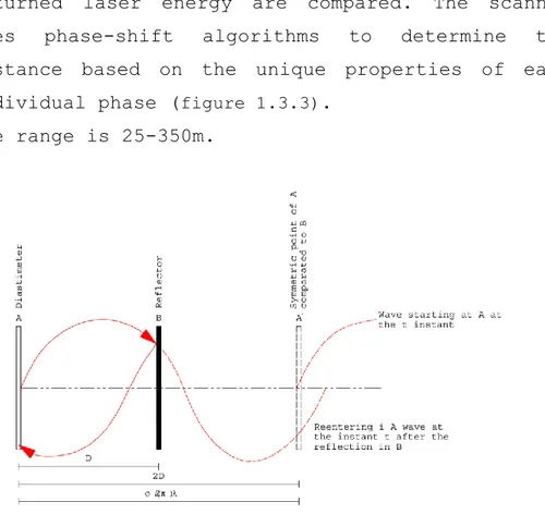
Phase based: the emitted laser light is modulated into multiple phases and the phase shifts of the
41
returned laser energy are compared. The scanner uses phase-shift algorithms to determine the distance based on the unique properties of each individual phase (figure 1.3.3).
The range is 25-350m.
Figure 1.3.3: Principle of a Phase based laser scanner.
Let us consider, as an example the case of a wave with a wavelength (λ) and suppose we want to measure, using this wave, a distance of less than λ/2. The wave, after covering the distance D, is reflected on the opposite end and goes back to the starting point. The phase shift measured between the transmitted wave and the received one will be a function of the distance D. Let A be the emission point and B the point of reflection of the wave.
42
Let A' be the symmetric point of A with respect to B (which is then 2D distant from A). The distance D is: D =2πφ ·λ2+ nλ2 → D = L + nλ2 (1.3.2) where: f = frequency φ = phase shift λ = wavelength = c/f c = velocity of propagation n = ambiguity
To measure a distance with a phase-based distance meter, it is therefore necessary to measure the phase shift φ and evaluate, without error, the integer number of half wavelengths.
Laser scanner measurements
The procedure for determining the coordinates of a point is distinct in two steps: data acquisition and calculation of the position.
Data acquisition involves three tasks (system calibration, georeferencing, measurement); the calculation of the position is obtained by data processing, which involves several steps: filtering and
43
deleting of features not belonging to the object; narrowing of the data; coordinate transformation and interpolation.
The greatest strengths of the laser scanner are: high speed and degree of automation; the survey is practically not affected by light conditions; very accurate three-dimensional geometric information; evaluation of the different reflectance values and, thus, possibility of evaluating the type of material constituting the detected object; possibility of integrating the survey with orthophotos or photos; possibility, through the analysis of the virtual model 3D, of visualizing and studying the object in terms of different aspects.
The accuracy of the laser scanner is directly affected by [Godin et al., 2001; Lichti et al., 2002; Voegtle et al., 2008; Beraldin et al., 2007]:
the quality of the internal device that performs the measurement;
the characteristics of the scanned material and scene, in terms of reflection, light diffusion and absorption (amplitude response);
the orientation and the local shape of the surface struck by the laser;
the characteristics of the working environment; the coherence of the backscattered light (phase
44
the chromatic content of the scanned material (frequency response).
When radiation hits the surface of a real body, also called gray body, it is partially absorbed by the body, in part reflected by the surface and in part transmitted. The following dimensionless coefficients can be defined (varying between 0 and 1), which measure the interactions between energy and matter: Absorptivity (): the ratio EA/EI between absorbed and incident energy; Reflectivity (): the ratio ER/EI between the reflected energy and the incident energy; Transmissivity (): the ratio ET/EI between the transmitted and the incident energy.
Generally, the perfectly smooth surfaces reflect in a specular way, those wrinkled behave as perfect Lambertian reflectors, i.e. the direction of reflection is independent of that of incidence. Normally, the real surfaces do not behave as surfaces which are perfectly specular nor perfectly Lambertian surfaces but rather show an intermediate behavior (figure 1.3.4).
Figure 1.3.4: Specular, diffuse (Lambertian) and spread reflection from surface.
45
Data Acquisition
The laser scanner, once centered on a place and leveled, scans the desired object and returns its digital model in the form of a cloud of points. The design phase of the scan, a proper acquisition of the photographic images if a mapping of the photos on the 3D model is required, and the proper disposition of the eventual targets are essential steps for correct surveying [Sgrenzaroli and Vassena, 2007]. The project of a laser scan survey can be performed considering the model of the used laser (precision, maximum range, acquisition rate, field of view), the subject you want to detect (the geometry and the size of the object) and the environment in which you can find the subject.
To correctly perform a survey one must:
scan in multiple locations: the choice of the number of scans depends on the field of view of the scanner.
place targets inside the area detected or on the object to be detected, in order to ensure the geo-referencing of scans and allow their union. From every point of the scan at least 3 well positioned targets must be visible. The target can be of various types and vary in shape, size, and material; these features ensure that the target can be identified automatically by the acquisition software supplied with the instrument.
46
if it is not possible to position artificial targets, one can use features recognizable on the scanned object [Gressin et al., 2012; Jaw and Chuang, 2008; Chillemi and Giacobbe, 2007]; features can be flat elements (stains, paintings, changes of the plaster) or spatial discontinuities (edges, holes). In other cases, it may be possible to replace the targets with a prism to be measured from a total station or with a GNSS receiver. Targets, prisms or antennas should be scanned at high resolution.
reduce shadows and occlusions: the maximum visibility of the area to be detected must be guaranteed by reducing the phenomena of shadows due to the presence of objects, undercuts, etc.
take into account the angle of acquisition: the quality of 3D points obtained by the laser scanner is also a function of the angle at which the laser beam is incident on the surface to scan.
have a good overlap between the scans to ensure the completeness of the 3D model, avoiding shadows and occlusions, and a good union of the scans in the case of use of a targetless registration.
try to have a homogeneous resolution scans in order to ensure the homogeneity of the geometric model both in terms of accuracy and of "density" of the point cloud.
47
Each laser scanner is equipped with a software designed specifically for the management of the acquisition phase. In general, these programs allow the definition of the general parameters of the acquisition (step scan, scan area), the real-time visualization of the results of the acquisition by a series of clouds of points, coloured in order to evidence the distances measured, and any RGB image recorded during the acquisition. After scanning, the operator can observe the acquired points in the monitor, change the point of view of the scan and move in the acquired point cloud in order to check its completeness.
Data Processing
The software for scans processing, as well as allowing the control and management of data acquisition, allows the pre-treatment of the acquired data (data cleaning, noise reduction, filtering and registration of point clouds), meshing (surface reconstruction, hole filling, smoothing), integration with other information (texturing), georeferencing and the extraction and export of geometric information [Karbacher et al., 2001; Bernardini and Rushmeier, 2002; Remondino, 2003; Rüther et al., 2014; Gomes et
48 al., 2014].
The data cleaning and filtering operation is necessary because of: the partial reflection of the laser on the edges; the errors in the calculation of the distance due to the presence of materials with different reflectivity; the presence of erroneous points caused by very bright objects; the atmospheric effects. To these errors should be added the points caused by the reflection of background objects, reflections originated in the space between scanner and the object (trees or objects in the foreground, people moving or traffic) and multiple reflections of the laser beam.
Registration
Each scan is carried out from a different point: thus, the point cloud coordinates are referred to a different local Cartesian reference system. Each reference system is centered in the instrument and arbitrarily oriented: it derives from this that the various point clouds related to the same object are independent, without any geometric links known a priori.
Registration is the set of all the operations needed to define the parameters of rotation and translation
49
that allow us to refer the various clouds to a single reference system.
The reference systems are the Intrinsic Reference System (IRS), an interior reference system, centered to the instrument, that gives relative coordinates, and the System Object Reference, usually materialized through a series of Ground Control Points GCP) with known coordinates. GCP are natural points or artificial targets identified individually in the scan.
The transformation from the intrinsic reference system in a given scan in the reference object system is made through a 3D rigid roto-translation, whose parameters can be calculated on the basis of control points, whose coordinates are known in both systems [Crosilla and Beinat et al., 2003].
The recording techniques based on the use of points, pre-signalized or not, assume that adjacent scans have a sufficient degree of overlap, not less than 30%, and that within this range there exist pre-signalized points, or directly detectable in the point clouds, of sufficient number to ensure the estimation of the parameters of the spatial transformation, which, as is known, is based on the following equations:
( X1 Y1 Z1 ) = ( Xu Yu Zu ) + 𝐑 · ( X2 Y2 Z2 ) (1.3.3)
50
where X1, Y1, Z1 are the coordinates in the reference system of the first scan, X2, Y2, Z2 the coordinates in the reference system of the second scan, Xu, Yu, Zu the coordinates of the origin of the reference system of the second scan, and R the rotation matrix that rotates the axes of the reference system of the second scanning by making them parallel to those of the reference system of the first scan.
The relationship that links together the different scans can be defined in a direct way already during the acquisition of the measures, or it can be derived in an indirect way acting analytically on the 3D numerical models produced for each scan.
For the direct alignment, one must detect the position and the attitude of the instrument for each acquisition. If this is mounted on a mobile vehicle, the displacement and the variation of attitude between the different scanning positions must be continously derived by means of auxiliary mechanical devices, like odometers, or by GPS receivers, coupled with inertial systems.
With regard to the indirect alignment, two are the procedures mainly used for the alignment: by using targeted or natural points or by iterative calculations.
One of the most popular iterative methods, still implemented in most commercial software used for the
51
management and processing of 3D data, is the Iterative Closest Point (ICP) algorithm, developed by Besl and McKay [Besl and McKay, 1992].
The ICP algorithm is used to align two point clouds; it is pair-wise based, and applies, iteratively, a roto-rigid translation in space to one of the two clouds, considered the mobile one, so that it overlaps in the best possible way to another cloud, considered the fixed one. The method is called point-to-point, as opposed to the point-plan method developed by Chen and Medioni [Chen and Medioni, 1991]. In both methods, registration is made through the search for the minimum of an objective function.
In the first method, point to point (Figure 1.3.5), this function is the sum of the squares of the Euclidean distances of the corresponding points of the clouds. The corresponding points are defined as the couple formed by a point of a cloud and the nearest one belonging to the opposite cloud.
Figure 1.3.5: Point to point method [Bernardini and Rushmeier, 2002].
52
The algorithm proceeds in this way: given two surfaces, P and Q, to be aligned, a point belonging to P is considered, named p, and you search for a particular point of Q, said corresponding point q, which coincides with the closest point (point at minimum distance); in practice, for each point of the mobile cloud, the points within the fixed cloud are found, contained within a sphere of a given radius σ (multiple of a parameter entered by the user) and of these the closest one is considered, which will be the corresponding point. Such a parameter in the literature is conventionally estimated as twice the average distance of the points of a cloud; however, in the case of a severe misalignment, it will have to be increased accordingly.
The searched points are found by defining the Closest Point Operator C:
C: P Q / ∀p∈P ∃ q∈Q : min p-q < σ (1.3.4)
Once this operation has been performed for all points of the moving cloud, the rigid rototranslation of the cloud is found, that minimizes the sum of the squared distances. To this aim, after creating the couples, one can proceed to the minimization of the function:
e = ∑ ‖qN i− (Rpi+ T)‖2
![Figure 1.3.1.1 Illustration of interaction of the laser pulse with different target, the digitization process, and target extraction by FWA [Pfennigbauer e Ullrich, 2008]](https://thumb-eu.123doks.com/thumbv2/123dokorg/2875826.9839/73.892.162.717.162.804/figure-illustration-interaction-different-digitization-extraction-pfennigbauer-ullrich.webp)
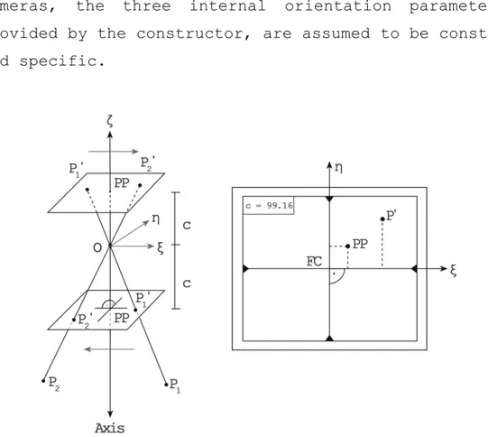
![Figure 1.4.4: Relationship between the coordinates of image points and object-points [Kraus, 1994]](https://thumb-eu.123doks.com/thumbv2/123dokorg/2875826.9839/85.892.202.706.289.838/figure-relationship-coordinates-image-points-object-points-kraus.webp)