A restricted composite likelihood approach to modelling Gaussian geostatistical data

A restricted composite likelihood approach to

modelling Gaussian geostatistical data

C.K. Mutambanengwe1,∗, C. Faes1and M. Aerts1

1 _{Interuniversity Institute for Biostatistics and Statistical Bioinformatics, Universiteit Hasselt,}

Marte-larenlaan 42, 3500 Hasselt, Belgium; chenjerai.mutambanengwe@uhasselt.be, christel.faes@uhasselt.be, marc.aerts@uhasselt.be

∗_{Corresponding author}

Abstract. Composite likelihood methods have become popular in spatial statistics. This is mainly due to the fact that large matrices need to be inverted in full maximum likelihood and this becomes computationally expensive when you have a large number of regions under consideration. We intro-duce restricted pairwise composite likelihood (RECL) methods for estimation of mean and covariance parameters in a Gaussian random field, without resorting back to the full likelihood. A simulation study is carried out to investigate how this method works in settings of increasing domain as well as in-fill asymptotics, whilst varying the strength of correlation. Preliminary results showed that pairwise composite likelihoods tend to underestimate the variance parameters, especially when there is high correlation, while RECL corrects for the underestimation. Therefore, RECL is recommended if interest is in both the mean and the variance parameters.

Keywords. Composite likelihood; REML; Spatial dependence; Effective sample size.

1

Introduction

Statistical problems that arise from the collection of spatial point-referenced data are complicated as a result of the spatial autocorrelation. If ignored, the data analysis can lead to erroneous conclusions. Weighted least squares (WLS) has been used to estimate variograms and semivariograms in spatial data. No distributional assumptions are made concerning the spatial process defined. However, this method relies on choices made for lag distances between points, as well as the lag tolerances [3]. The methods of maximum likelihood (ML) or restricted maximum likelihood (REML) theoretically yield an optimal estimator but require a full specification of the probabilistic model. This involves inversion of matrices for each likelihood function calculated, which quickly increases the computational effort as the number of observations increases, even for simple likelihoods. To reduce this burden, composite likelihood (CL) methods have been considered. A recent review of CL methods is given by [7]. The idea of CL is to

C.K. Mutambanengweet al. Restricted composite likelihood

replace the likelihood by a simpler function, constructed from summing over the contributions of the likelihoods on subsets of the data, as such leading to a simpler function to be evaluated, but at the cost of efficiency loss. This idea was proposed by [1] in the context of spatial data, and called pseudo-likelihood. Later, it was called composite likelihood by [6]. We will focus on the specification of the CL for spatial geostatistical data based on pairwise differences, as done by [3], and on pairwise likelihood contributions as defined in [7]. When variance parameters are of interest, for example interest in the variogram, ML estimation is known to be biased as a result of the loss in degrees of freedom. This bias can be reduced substantially by using REML. The same applies for the composite likelihood estimation of the covariance parameters. In this paper, it will be investigated how the composite likelihood method can be penalised in a similar way as in REML, in order to reduce bias in the variance parameter. The proposed method will be called the restricted composite likelihood method (RECL).

2

Methods

Let Z be a random variable from a Gaussian random field with observations {Zi; i = 1, ..., n} recorded

at sites si such that Z ∼ N(µ, C(σ2, ρ)). The mean µ = Xβ is a function of the covariates X and

associated regression coefficients β. The spatial dependence in the data is captured by the variance-covariance matrix C(σ2, ρ), where σ2 is the variance of the spatial process and ρ is a measure of the correlation between any two sites determined by the distance between them. This second-order sta-tionary process has semi-variogram γ(si, sj) = 1₂var(Z(si) − Z(sj)). The most popular semivariogram

is the Matérn class, which has the special case of the exponential semivariogram, parametrized as γ(si, sj; φ) = c0+ σ2(1 − ρ|si−sj|) where φ = (c0, σ2, ρ). The parameters c0and σ2are called the nugget

and the sill, respectively, and c0+ σ2 represents the process variance, ρ is the spatial dependence. Two

types of composite likelihood methods are considered: (1) pairwise differences (CL1), (2) marginal

pair-wise method (CL2). The CL1 method treats the mean µ as a nuisance parameter and does not estimate

it. When µ needs to be estimated, the latter approach will result in biased estimates for the covariance function. In the likelihood framework one often uses REML estimation for the variance parameters, which are no longer biased downwards [5]. Similar as with REML, a penalisation is added to the (log) composite likelihood function to formulate the RECL as

RECL= n−1

∑

∑

∑

∑

where Xi jis the covariate matrix for the pair (i, j) (and is a column of 1’s if a constant mean is assumed),

Ci j is the variance-covariance matrix between pair (i, j), with weights w = n

0

n(n−1), n the number of

locations and n0denoting the effective sample size (ESS) given by n0= n2

∑ni=1∑nj=1ρ|si−s j|

[4]. The weights w are (1) set equal to 1 (RECL1), or estimated by setting ρ equal to (2) known ρ (RECL2), (3)bρ from CL1 (RECL3) and (4)bρ from CL2(RECL4).

3

Simulation study

A simulation study is carried out to explore the properties of our estimators in a similar fashion to [3]. Data are simulated on an 8x8 regular grid with unit interval spacing, and on two 15x15 grids obtained by halving the grid spacings (infill asymptotics) and doubling the grid spacing (increasing

C.K. Mutambanengweet al. Restricted composite likelihood

domain asymptotics). ρ was varied to represent relatively weak, moderate, and strong levels of spatial dependence by setting the distance at which values become approximately uncorrelated to be 0.2, 0.5, and 0.8 times the maximum distance over the domain S. The variance parameter σ2 was set at 1, the mean µ was set at 3, and it is assumed that c0= 0. The simulation is repeated 500 times.The results for

moderate dependence are summarised in Figure 1 which shows box plots of the σ2, ρ and µ parameters for eight estimation methods. The horizontal line corresponds with the true underlying value. The ML and REML estimates that use the full likelihood have better estimates than all other methods, but have the drawback that it is computationally intensive. CL1also works very good, but treats the mean

parameters as nuisance, while they could be of interest in practice. CL2 and RECL1 perform similar

to each other, with bias in mainly the parameter ρ. Inclusion of weights greatly improved the point estimates. Weighting using the correlation estimate from the differences method is recommended in practice, since true correlations are never known. Note that all models perform relatively well when the correlation is weak. However, larger differences are observed as the correlation gets stronger, especially for the ρ parameter, with the proposed method providing a good correction with the least bias compared to the other composite likelihood methods.

● ● ● ● ● ● ● ● ● ● ● ● ● ● ● ● ● ● ● ● ● ● ● ● ● ● ● ● ● ● ● ● ● ● ● ● ● ● ● ● ● ● ● ● ● ● ● ● ● ● ● ● ● ● ● ● ● ● ● ● ● ● ● ● ● ● ● ● ● ● ● ● ● ● ● ● ● ● ● ● ● ● ● ● ● ● ● ● ● ● ● ● ● ● ● ● ● ● ● ● ● ● ● ● ● ● ● ● ● ● ● ● ● ● ● ● ● ● ● ● ● ● 1 2 3 4 5 6 7 8 0.0 0.5 1.0 1.5 2.0 2.5 3.0 Variance 8x8 ● ● ● ● 1 2 3 4 5 6 7 8 0.0 0.2 0.4 0.6 0.8 1.0 Correlation ● ● ● ● ● ● ● ● ● ● ● ● ● ● 1 2 3 4 5 6 7 8 1 2 3 4 5 Intercept ● ● ● ● ● ● ● ● ● ● ● ● ● ● ● ● ● ● ● ● ● ● ● ● ● ● ● ● ● ● ● ● ● ● ● ● ● ● ● ● ● ● ● ● ● ● ● ● ● ● ● ● ● ● ● ● ● ● ● ● ● ● ● ● ● ● ● ● ● ● ● ● ● ● ● ● ● ● ● ● ● ● ● ● ● ● ● ● ● ● ● ● ● ● ● ● ● ● ● ● ● ● ● ● ● ● ● ● ● ● ● ● ● ● ● ● ● ● ● ● ● ● ● ● ● ● ● ● ● ● ● ● ● ● ● ● ● ● ● ● ● ● ● ● ● ● ● ● ● ● ● ● ● ● ● ● ● ● ● ● ● ● ● ● ● ● ● ● ● ● ● ● ● ● ● ● ● ● ● ● ● ● ● ● ● ● ● ● ● ● ● ● ● ● ● 1 2 3 4 5 6 7 8 0.0 0.5 1.0 1.5 2.0 2.5 3.0 15x15 infill 1 2 3 4 5 6 7 8 0.0 0.2 0.4 0.6 0.8 1.0 ● ● ● ● ● ● ● ● ● ● ● ● ● ● ● ● ● ● ● ● ● ● 1 2 3 4 5 6 7 8 1 2 3 4 5 ● ● ● ● ● ● ● ● ● ● ● ● ● ● ● ● ● ● ● ● ● ● ● ● ● ● ● ● ● ● ● ● ● ● ● ● ● ● ● ● ● ● ● ● ● ● ● ● ● ● ● ● ● ● ● ● ● ● ● ● ● ● ● ● ● ● ● ● ● ● ● ● ● ● ● ● ● ● ● ● ● ● ● ● ● ● ● ● ● ● ● ● ● ● ● ● ● ● ● ● ● ● ● ● ● ● ● ● ● 1 2 3 4 5 6 7 8 0.0 0.5 1.0 1.5 2.0 2.5 3.0 15x15 increasing domain ● ● ● ● ● ● ● ● ● ● ● ● ● ● ●●● ● ● ● ● ● ● ● ● ● ● 1 2 3 4 5 6 7 8 0.0 0.2 0.4 0.6 0.8 1.0 ● ● ● ● ● ● ● ●●●● ● ● ● ● ● ● ● ● ● ● ● ● ● ● ● ● ● ● ● ● ● ● ● ● ● ● ● ● ● ● ● ● ● 1 2 3 4 5 6 7 8 1 2 3 4 5

Figure 1: Box plots of σ2, ρ and µ parameters for moderate dependence settings. Estimation methods: 1: ML; 2: REML; 3: CL1; 4:CL2; 5: RECL1; 6: RECL2; 7: RECL3; and 8: RECL4.

4

Conclusions

In conclusion, penalization seems important also in composite likelihood methods, and the choice of weights is key in obtaining good results. Weighting with estimated effective sample size shows better

C.K. Mutambanengweet al. Restricted composite likelihood

σ2 ρ µ

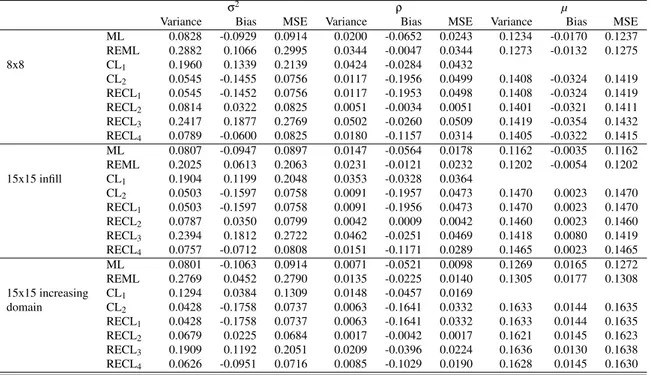
Variance Bias MSE Variance Bias MSE Variance Bias MSE ML 0.0828 -0.0929 0.0914 0.0200 -0.0652 0.0243 0.1234 -0.0170 0.1237 REML 0.2882 0.1066 0.2995 0.0344 -0.0047 0.0344 0.1273 -0.0132 0.1275 8x8 CL1 0.1960 0.1339 0.2139 0.0424 -0.0284 0.0432 CL2 0.0545 -0.1455 0.0756 0.0117 -0.1956 0.0499 0.1408 -0.0324 0.1419 RECL1 0.0545 -0.1452 0.0756 0.0117 -0.1953 0.0498 0.1408 -0.0324 0.1419 RECL2 0.0814 0.0322 0.0825 0.0051 -0.0034 0.0051 0.1401 -0.0321 0.1411 RECL3 0.2417 0.1877 0.2769 0.0502 -0.0260 0.0509 0.1419 -0.0354 0.1432 RECL4 0.0789 -0.0600 0.0825 0.0180 -0.1157 0.0314 0.1405 -0.0322 0.1415 ML 0.0807 -0.0947 0.0897 0.0147 -0.0564 0.0178 0.1162 -0.0035 0.1162 REML 0.2025 0.0613 0.2063 0.0231 -0.0121 0.0232 0.1202 -0.0054 0.1202 15x15 infill CL1 0.1904 0.1199 0.2048 0.0353 -0.0328 0.0364 CL2 0.0503 -0.1597 0.0758 0.0091 -0.1957 0.0473 0.1470 0.0023 0.1470 RECL1 0.0503 -0.1597 0.0758 0.0091 -0.1956 0.0473 0.1470 0.0023 0.1470 RECL2 0.0787 0.0350 0.0799 0.0042 0.0009 0.0042 0.1460 0.0023 0.1460 RECL3 0.2394 0.1812 0.2722 0.0462 -0.0251 0.0469 0.1418 0.0080 0.1419 RECL4 0.0757 -0.0712 0.0808 0.0151 -0.1171 0.0289 0.1465 0.0023 0.1465 ML 0.0801 -0.1063 0.0914 0.0071 -0.0521 0.0098 0.1269 0.0165 0.1272 REML 0.2769 0.0452 0.2790 0.0135 -0.0225 0.0140 0.1305 0.0177 0.1308 15x15 increasing CL1 0.1294 0.0384 0.1309 0.0148 -0.0457 0.0169 domain CL2 0.0428 -0.1758 0.0737 0.0063 -0.1641 0.0332 0.1633 0.0144 0.1635 RECL1 0.0428 -0.1758 0.0737 0.0063 -0.1641 0.0332 0.1633 0.0144 0.1635 RECL2 0.0679 0.0225 0.0684 0.0017 -0.0042 0.0017 0.1621 0.0145 0.1623 RECL3 0.1909 0.1192 0.2051 0.0209 -0.0396 0.0224 0.1636 0.0130 0.1638 RECL4 0.0626 -0.0951 0.0716 0.0085 -0.1029 0.0190 0.1628 0.0145 0.1630

Table 1: Variance, Bias and MSE estimates for moderate dependence setting.

improvement from marginal pairwise models. The computation time is also greatly reduced when using neighbouring pairs instead of all pairs, which is desirable when sample sizes are large and full likelihood methods fail or take too much time. This is synonymous with weighting schemes used by, for example, [2], and the results obtained are very similar as to when all pairs are used. Preliminary analyses have been attempted including covariates in the estimation. The results suggest that the mean parameters are still estimated very well but more research is being done to understand how this affects the variance parameters. There is also continuing work to explore variance estimation for the proposed methods.

References

[1] Besag, J. E. (1974). Spatial interaction and the statistical analysis of lattice systems (with discussion). Journal

of the Royal Statistical Society, Series B34, 192–236.

[2] Bevilacqua, M., and Gaetan, C. (2014). Comparing composite likelihood methods based on pairs for spatial Gaussian random fields. Statistics and Computing. In press.

[3] Curriero, F.C., and Lele, S.R. (1999). A Composite Likelihood Approach to Semivariogram Estimation. Journal of Agricultural, Biological, and Environmental Statistics. 4(1), 9–28.

[4] Fortin, M.J., and Dale, M.R.T. (2005). Spatial Analysis: A Guide for Ecologists.. Cambridge University Press.

[5] Harville, D.A. (1974). Bayesian inference for variance components using only error contrasts. Biometrika. 61, 383–385.

[6] Lindsay, B.G. (1988). Composite likelihood methods. Contemporary Mathematics. 80, 221–240.

[7] Varin, C., Reid., N., and Firth, D. (2011). An overview of composite likelihood methods. Statistica Sinica. 21, 5–42.