www.biogeosciences.net/6/1783/2009/
© Author(s) 2009. This work is distributed under the Creative Commons Attribution 3.0 License.
Biogeosciences
Interactions among vegetation and ozone, water and nitrogen fluxes
in a coastal Mediterranean maquis ecosystem
G. Gerosa1, A. Finco1, S. Mereu3, R. Marzuoli2, and A. Ballarin-Denti1
1Dip. to di Matematica e Fisica, Universit`a Cattolica del S.C., via Musei 41, 25121 Brescia, Italy 2CRINES, via Galilei 2, Curno, Italy
3Dip. to di Biologia Vegetale, Universit`a La Sapienza, via Fermi 1, Rome, Italy Received: 3 December 2008 – Published in Biogeosciences Discuss.: 29 January 2009 Revised: 28 April 2009 – Accepted: 11 August 2009 – Published: 26 August 2009
Abstract. Ozone, water and energy fluxes were measured
over a Mediterranean maquis ecosystem from 5 May until 31 July 2007 by means of the eddy covariance technique. Ad-ditional measurements of NOxfluxes were performed by the aerodynamic gradient technique. Stomatal ozone fluxes were obtained from water fluxes by a Dry Deposition Inferential Method based on a big leaf concept.
The maquis ecosystem acted as a net sink for ozone. The different water availability between late spring and summer was the major cause of the changes observed in stomatal fluxes, which decreased, together with evapotranspiration, when the season became drier.
NOx concentrations were significantly dependent on the local meteorology. NOxfluxes resulted less intense than the ozone fluxes. However an average upward flux of both NO and NO2was measured.
The non-stomatal pathways of ozone deposition were in-vestigated. A correlation of non-stomatal deposition with air humidity and, in a minor way, with NO2fluxes was found.
Ozone risk assessment was performed by comparing the exposure and the dose metrics: AOT40 (Accumulated dose over a threshold of 40 ppb) and AFst1.6 (Accumulated
stom-atal flux of ozone over a threshold of 1.6 nmol m−2s−1). AOT40, both at the measurement height and at canopy height was greater than the Critical Level for the protection of forests and semi-natural vegetation (5000 ppb h) adopted by UN-ECE. Also the AFst1.6 value (12.6 mmol m−2PLA,
Pro-jected Leaf Area) was higher than the provisional critical dose of 4 mmol m−2PLA for forests. The cumulated dose showed two different growth rates in the spring and in the summer periods, while the exposure showed a more irregular behavior in both periods.
Correspondence to: G. Gerosa
1 Introduction
The toxicity of ozone for plants has been widely documented over the past twenty years (Benton et al., 2000; Sk¨arby et al., 1998). Even when ozone does not bring to visible damage on the leaf lamina (Bermejo et al., 2003; Novak et al., 2008; Marzuoli et al., 2008), it remains a cause for physiological alterations and a general loss in Net Primary Productivity (NPP) (Felzer et al., 2004; King et al., 2005).
Mediterranean ecosystems, because of their climatic con-ditions and their proximity to anthropic sources of ozone pre-cursors, are among the most exposed ecosystems to this pol-lutant (Paoletti et al., 2006). The EMEP model estimated for the Mediterranean areas an exposure between 40000 and 60 000 ppb h (on a six months basis, April–September) for the year 2000 (Simpson et al., 2007; Emberson et al., 2007), a value exceeding from 8 to 12 times the critical level of 5000 ppb h set by UN-ECE for the protection of forests and seminatural vegetation. The year 2000 was chosen as the reference year since all the papers published by the au-thors of the model and its further developments and adjust-ments (EMEP-DO3SE model) have been referred to the same year/dataset.
Nevertheless field observations never reported a particu-larly strong plant injury (Bussotti and Gerosa, 2002; Bussotti et al., 2006, Paoletti et al., 2006), thus questioning the sound-ness of the exposure concept applied to ozone risk assess-ment. However, the lack of visible injuries in the Mediter-ranean vegetation could be due to extremely efficient physio-logical and biochemical defense mechanisms of these plants to oxidative stress as some experiments in controlled envi-ronments revealed (Nali et al., 2004; Elvira et al., 2004).
Among the physiological responses, stomatal regulation plays an important role because the reduction of the stom-atal conductance due to the water limitation typical of the
1784 G. Gerosa et al.: Ozone, water and nitrogen fluxes in a maquis ecosystem
Mediterranean summer implies a lowering of the ozone up-take by plant and hence of the effects of this pollutant.
Because of the crucial role of stomata in regulating the dose absorption process, the cumulative ozone flux (AFstY)
has been chosen by UN-ECE as a more reliable ozone risk index then AOT40 (Musselmann et al., 2006; Karlsson et al., 2007, Matyssek et al., 2007). This index is based on the accumulation of stomatal fluxes over a threshold (Y) which accounts for the biochemical detoxification mech-anisms. This threshold value has been provisionally set to 1.6 nmol m−2s−1 (Karlsson et al., 2004) for forests and 6 nmol m−2s−1for crops (Pleijel et al., 2004), however the meaning and usefulness of Y is still debated and discussed in the UN-ECE effects-based community. Despite the acknowl-edged better biological soundness of AFstY over AOT40
(Matyssek et al., 2007, Karlsson et al., 2007) AOT40 is still widely used since field measurements of AFstY are difficult.
The calculation of AFstY from the observation in the field, in fact, requires the setting up of non-routinely monitoring systems, such as 3-D sonic anemometers and fast gas analy-sers for the Eddy Covariance micrometeorological technique (Keronen et al., 2003), branch chambers or similar and sap flow systems, which require the use of not completely stan-dardized complex equipment. On the contrary the evaluation of AOT40 requires only ambient air ozone concentrations which are routinely monitored by the national or regional survey networks.
Moreover, the derivation of bulk stomatal flux from mi-crometeorological measurements requires the application of dry deposition inferential methods, data checking and gap-filling techniques which may not be completely automated. As a consequence, flux based risk assessments is mostly per-formed with the aid of models, such as the deposition mod-ule DO3SE (Emberson et al., 2007; Ashmore et al., 2007) included in the EMEP model rather than a network of ozone flux monitoring stations.
Unfortunately, DO3SE has been validated mostly with ob-servations of total O3flux and stomatal conductance (gs) in ecosystem types which are representative of the Central and Northern Europe (e.g. Tuovinen et al., 2001). In Mediter-ranean conditions only one comparative study on wheat (Tuovinen et al., 2004) has been conducted in Italy and, to date, validation and comparison are still missing for an ev-ergreen Mediterranean forest or the Mediterranean maquis. In fact it is important to test the model in conditions where high ozone concentrations can occur with high soil and at-mospheric water deficits (Emberson et al., 2005).
Moreover a great amount of the ozone deposited to the ecosystems can be depleted prior to be absorbed by stom-ata. This non-stomatal deposition have been reported by many authors (e.g. van Pul and Jacobs, 1994; Fowler et al., 2001; Altimir et al., 2004, 2006; Gerosa et al. 2003, 2004, 2009a; Cieslik 2009a) and it was attributed to ozone destruc-tion over plant and soil surfaces (van Pul and Jacobs, 1994), thermal decomposition mediated by solar radiation (Fowler
et al., 2001; Rond´on, 1993), gas phase reaction with biogenic volatile organic compounds (Kurpius and Goldstein, 2003) or with nitric oxide emitted by soils (Dorsey et a., 2004; Pi-legaard et al., 1999), reaction with air humidity and water films (Altimir et al., 2004; 2006). However, the nature of this deposition is still not completely clear and further re-search is needed. Nevertheless the knowledge of the amount of ozone deposited by non-stomatal pathways is important for the ozone risk assessment since it affects the ozone fluxes to the ecosystems as well as the ozone concentrations at the leaf level thus leading to the ozone uptake by stomata.
This article is aimed to the analysis of the ozone flux dy-namics and their interaction with NOxin a water limited en-vironment during the dry season, and to offer a dataset of measurements suitable for model calibration and validation. It is also aimed at assessing the ozone risk for a Mediter-ranean maquis ecosystem, by the measurement of the dose actually absorbed by the vegetation through stomata and its comparison with AOT40.
2 Materials and methods
Measurements were performed from 5 June to 31 July 2007 in a coastal Mediterranean maquis at Castelporziano, Italy (N 41◦40049.300, E 12◦23030.600).
Due to the poorness of the sandy soil the vegetation of this site do not develop completely. The ecosystem is kept in a dynamic equilibrium between two different succes-sion stages of the maquis: low maquis and medium maquis (corresponding to low matorral and middle matorral sensu Tomaselli 1981). Ninety percent of the ground is covered by 6 main species: Quercus ilex, Arbutus unedo, Rosmarinus
officinalis, Cistus spl, Phyllirea latifolia, Erica multiflora.
The average height of vegetation was around 120 cm. About 90% of vegetation falls in a range plus or minus 30 cm from the average height, while the remaining 10% was char-acterised by the occurrence of few Quercus ilex and
Arbu-tus unedo individuals which were on average 50 cm higher.
More details on the measuring site can be found in Fares et al. (2009)
Two different techniques were used to measure turbulent fluxes of energy and matter: the eddy covariance technique and the gradient approach. A Dry Deposition Inferential Method approach (Wesely and Hicks, 2000; Gerosa et al., 2003, 2004, 2005) was then applied to calculate the ozone stomatal fluxes and the toxicological dose absorbed by the ecosystem.
2.1 Instrumentation
Sensible and latent heat fluxes as well as ozone fluxes were measured using the eddy covariance technique (Swinbank, 1951; Hicks and Matt, 1988). An ultrasonic anemometer (USA-1, Metek, Elmshorn, Germany), a CO2/H2O open path
fast sensor (LI-7500, LI-COR, Lincoln, Neb., USA) and a fast ozone analyser (COFA, Ecometrics, Italy) were mounted on the top of a 3.8 m tall scaffold.
One net radiometer (NR lite, Kipp & Zonen, Holland), one PAR meter (190SA, LI-COR, Lincoln, Neb., USA) and a temperature and relative humidity probe (50Y, Campbell Scientific, Shepshed, UK) were placed at the same height than the anemometer. An additional reference O3 analyzer (S-5014, SIR, Spain), sampling air at the top of the scaffold near the fast ozone sensor, was also used.
NO and NO2fluxes were measured by a NOxanalyzer (S-2308, SIR, Spain) using the gradient approach, measuring the nitrogen oxides concentrations alternatively at two different heights by means of an electro-valve switching system con-trolled by a computer with a LabView (National Instruments, Austin, Tx, USA) software. The two sampling points were chosen at 3.8 m and 1.3 m.
The measuring site was equipped with additional instru-mentation to better describe the temperature and humidity profile, the soil water status, the energy fluxes and the mi-croclimate of the area: two additional temperature and rel-ative humidity probes (50Y, Campbell Scientific, Shepshed, UK) at 1 m and 0.1 m; three soil heat flux plates, (HFP01SC, Hukseflux, Delft, Holland); three TDR reflectometers (C616, Campbell Scientific, Shepshed, UK); one rain gauge (52202, Young/Campbell Scientific, Cambridge, UK); one barometer (PTB101B,Vaisala, Finland); three leaf temperature probes (Pt100, DeltaT, UK) and two surrogate leaves (237, Camp-bell Scientific, UK) to measure leaf wetness.
The latter sensors are circuit boards of 6×8 cm epoxy-fiberglass green coloured resin with interlacing gold-plated fingers. Condensation on the sensors lowers the resistance between the fingers, which is measured by the datalogger. Sensors were not coated with latex paint and were mounted horizontal to the soil at 1 m height, with the grids facing up, just over two Holm oak bushes 3 m away from the measuring tower. Despite the Campbell 237 manual indicate a 150 K as a wetness/dryness threshold, in order to enhance the sen-sor sensitivity and promptness a very high dryness threshold of 6 M was set, so all the conditions in which a resistance value was less than 6 M were classified as wet canopy con-ditions.
Fast sensors were sampled at 20 Hz by a computer with a customised software written in Delphi 5.0 (Borland). Slow sensors were sampled every 15 seconds and data were collected by a datalogger (CR10x, Campbell Scientific, Shepshed, UK) equipped with a signal multiplexer device (AM16/32, Campbell Sci., UK), and data were averaged ev-ery 30 min.
2.2 Eddy-covariance
Eddy covariance is a turbulence based technique which states that fluxes are equal to the covariance between the vertical component of the wind (w) and the measured scalar
quan-tity. Originally developed by Swinbank (1951), it has been accurately described and widely used for gas exchange mea-surements (e.g. Stull, 1988; Kaimal and Finnigan, 1994; Fo-ken, 2008).
Under some conditions that have to be fulfilled (station-arity of the variables for which vertical fluxes are calcu-lated, horizontal homogeneity, absence of chemical sources and sinks between the measuring height and the exchanging surface, and average vertical wind component equal to zero; Gr¨unhage et al., 2000) vertical fluxes are constant with height and ozone, sensible and latent heat fluxes can be calculated as follows
FO3 =w
0C0 (ppb m/s) (1)
H = ρ cpw0T0 (W m−2) (2)
λE = λρ w0q0 (W m−2) (3)
where C is the ozone concentration (ppb), T the air temper-ature (◦C), q the specific humidity of the air (Kg vapor/Kg
air), ρ the air density (Kg m−3), λ the constant of water va-porization (J Kg−1K−1), and cp the specific heat of the air
(J Kg−1K−1). The primes (0) indicate fluctuations of each variable around their mean and the overbars represent ages over a chosen time period, in our case a 30 min aver-aging period. This period is short enough to separate syn-optic and diurnal variations from the turbulent data (van der Hoven, 1957), and long enough to include all turbulent fluc-tuations occurring in the atmospheric surface layer.
At the end of each 30 min averaging period, the fluctua-tions around the means were calculated after linear detrend-ing of the data series and a covariance matrix was calculated, i.e. the covariances between every considered parameter and each other. Then the covariance matrix was rotated following the three rotations suggested by McMillen (1988) in order to eliminate the advective components resulting from small non-homogeneities of the exchanging surface and an even-tual slight vertical tilt of the instrumentation.
In order to ensure a perfect synchronization of the data se-ries and to account for different instrumental delays, the data series of the variables acquired by fast sensors were lagged with successive steps of 0.05 s, with respect to the wind data series, until the calculated fluxes reached their maximum value. When a maximum flux value was not found within the 60th lag, the sample was recognized as not stationary and discarded.
2.2.1 Data selection
In addition to the previous method, the fulfillment of the sta-tionarity requirement has been checked by using the selec-tion criterion proposed by Dutaur et al. (1999). This crite-rion requires that fluctuations are calculated in two different ways: as the difference of the linear detrended series with the 30-min average, and as the difference with an instantaneous
1786 G. Gerosa et al.: Ozone, water and nitrogen fluxes in a maquis ecosystem
local running mean obtained by passing a mathematical R-C recursive filter (analogous of an electric circuit of a resistor and a capacitor in series) over the original time series. If the normalized absolute difference between the covariances calculated with the fluctuations obtained with the two meth-ods is below 1, the sample was considered as stationary and reliable. On the contrary, the sample was discarded.
Other data selection criteria were that the data capturing efficiency of each sample had to be greater than 85%, and that the canopy had to be completely dry. Only the data that passed these selections were used for successive analysis.
2.2.2 Calculation of stomatal fluxes by a Dry Deposition
Inferential Methodology
The deposition of a gas depends on many variables such as wind velocity, friction velocity, incoming radiation, temper-ature, surface type, etc. In the Dry Deposition Inferential Method approach (DDIM) the deposition surface is treated as a “big leaf” located at a height d+z0over the soil, where
dis the displacement height accounting for the canopy height
h(set to 2/3 of the h) and z0is the roughness length which accounts for the canopy roughness (set to 12/100 of h). Three main phases are considered in the deposition process: first of all the gas must overcome the aerodynamic resistance (Ra)
existing in the turbulent layers of the atmosphere above the studied surface; then the gas must move across the quasi-laminar sub-layer which is characterized by a molecular dif-fusion against the so-called sub-laminar resistance (Rb);
fi-nally, in order to reach the surface, the gas must overcome the resistance of the surface itself (Rc). The deposition flux of a
gas is hence considered as the analogous of a current flowing through a electric circuit composed by these three resistances in series. Their equivalent resistance is called total resistance (Rtot)and it is equal to the concentration of the gas at the measuring point divided by the deposition (i.e. <0) flux FO3:
Rtot=Ra+Rb+Rc=Czm/(−FO3) ∀FO3 <0 (4)
The aerodynamic resistance Ra was calculated using the
well known similarity relation introduced by Monin and Obukhov (1954), while the sub-laminar resistance Rb for
ozone was calculated following the general purpose parame-terization proposed by Hicks et al. (1987). The surface resis-tance Rcis hence obtained as a residual since Rtotis known,
because it is derived from directly measured entities (Czm
and FO3).
In order to estimate the fraction of gas penetrating through the stomata of plants, the surface resistance Rc (also called
the canopy resistance in ecology) is broken down into a stom-atal resistance and a non-stomstom-atal one mounted in parallel.
The stomatal resistance to ozone, RST, has been calculated
from the stomatal resistance to water evaporation Rwby
in-verting the Penmann-Monteith equation (Monteith, 1981) – i.e. by solving this equation for Rwsince all the other entities
are directly known from measurements- and by considering
the relative diffusivity ratio of ozone in air to that of water vapour (Massman, 1998), set equal to 0.61 following the av-erage T and P conditions at this site.
The non-stomatal resistance was calculated as a residual from Rc and RST, following the rules of the parallel
resis-tances. The stomatal ozone flux was hence obtained as
FST =
Rc
(Ra+Rb+Rc) RST
Czm (5)
Further details can be found in Gerosa et al. (2005).
Samples where the inferred values of Ra and Rb exceeded 10 000 s m−1 were rejected, because unrealistic. The same was done for samples where Rcresulted lower than 0 because
the sum of Ra and Rb exceeded the measured total
resis-tance to ozone (Rcwas obtained as a residual) or when RST
was not computable because the Penman-Monteith equation could not be inverted, e.g. when λE was not positive. A threshold value of 10 000 s/m was applied to the stomatal re-sistance when its value increased above this value assumed to be representative of the cuticular resistance.
Finally, in order to preserve a numerical coherence, if the estimation of one resistance failed, then all the sample were discharged, even though the values of the other resistances seemed reasonable.
2.2.3 Ozone dose and exposure
In this work both exposure and dose approaches were com-pared. The exposure was calculated as AOT40 for daylight hours only:
AOT40 = X
∀GlobRad≥50 W/m2
max(0; Cd+z0 −40) 1t (6)
where 1t is the averaging period for the ozone concentra-tion measurements (1 h). The concentraconcentra-tion at d+z0, recom-mended by the ICP modelling and mapping manual (2004), was calculated with the Dry Deposition Inferential Method (Gerosa et al., 2005):
Cd+z0 =Czm(1 − Ra/Rtot) (7)
The ozone dose received by the ecosystem in the whole mea-suring period (May–July) was calculated as AFst0 by
sum-ming up all the 30-min ozone stomatal fluxes Fst of the
pe-riod
AFst0 = X
max(0; Fst) 1t (8)
where 1t is the averaging period chosen for eddy covariance measurements.
The dose was also calculated as AFst 1.6:
AFst1.6 = X
max(0; Fst−1.6) 1t . (9)
where Fst is the stomatal ozone flux obtained by the DDIM,
1.6 nmol m−2s−1 is the UN-ECE detoxification threshold and 1t is the averaging period of the flux measurements.
2.2.4 Data gap-filling
The results presented in this paper rely on the measured data that fulfilled all the selection criteria. One unique exception has been made for the assessment of the exposure and the dose.
In fact, since both AOT40 and the ozone dose are cumula-tive metrics, a gap in ozone concentrations and ozone fluxes will result in an unavoidable underestimation of their values. To reduce such underestimation a gap-filling was per-formed. Gaps of no more than 3 consecutive 30-min averages were linearly interpolated, while large gaps were gap-filled with time series reconstructed by multiple linear regression based on available predictors as local meteorological param-eters and ozone concentrations from a nearby measuring sta-tion.
Gaps in stomatal fluxes could result also as a consequence from data rejection at the output of the DDIM process. In these cases stomatal fluxes were estimated by taking the av-erage stomatal fraction (the ratio between Fst and Ftot, based solely on measured data) at the corresponding half an hour, and by multiplying it by the available total ozone flux .
2.3 Gradient approach
The aerodynamic gradient has been widely used to estimate surface fluxes (Grunhage et al., 2000; Foken, 2008) since, unlike eddy covariance, it does not require fast analyzers. Here the turbulent diffusion coefficient for heat KH, that
takes into account also the vertical stability of the atmo-sphere, was easily available from eddy covariance data and applied to both nitric oxide and nitrogen dioxide fluxes, fol-lowing the similarity of the transport of each scalar entity found by Monin and Obhukhov (1954) (Stull, 1988; Mon-teith and Unsworth, 1990; Pal Arya, 1988). Nitrogen oxides fluxes were hence calculated for each half-hours as follows:
FNOx = −KH·1[NOx]/1z (10)
where NOxindicates the NO concentrations when calculat-ing the NO fluxes FNOand the NO2concentrations when cal-culating the NO2fluxes FNO2, 1 [NOx] is the mean
differ-ence of NO and NO2 concentrations between the two mea-suring heights z2and z1, and 1z is z2−z1, equal to 2.5 m in our case.
3 Results
A total of 4176 semi-hourly samples were gathered during the whole measuring period. The samples referred to com-pletely dry canopy conditions were 1894 (45.3%), because nearly all the samples between 8 p.m. and 8:30 a.m. were excluded due to the presence of dew on the leaves. This sub-dataset was further reduced by 16% because instrumental drawbacks (e.g. shut down, instrument breakings and substi-tutions), and by another 33.2% following the exclusion of the
data which did not fulfill the stationarity conditions. Hence the output of the DDIM analysis is based on the 50.8% of the data gathered from 8:30 a.m. to 8 p.m., except when explic-itly indicated.
In order to highlight different physiological traits, most of the results are split in two different periods: the first one from 5 May to 12 June (late spring) and the second one from 13 June to 31 July (summer).
3.1 Ozone concentrations and fluxes
The average ozone concentration at the measuring height was 32.6 ppb in the first period and 38.6 ppb in the second one. The overall average was 35.9 ppb and the maximum peak concentration was 107 ppb. Ozone concentrations were strongly influenced by the local meteorology: higher concen-trations were observed when the wind was blowing from the sea and lower concentrations downwind to the city of Rome. Ozone concentrations usually began to increase early in the morning, around 8 a.m. reaching their daily maximum in the first afternoon, and decreased to the lower nighttime values afterwards (Fig. 1). With the only exception of some days with high nighttime values, ozone concentrations showed a typical bell-shaped behavior.
On the contrary, the total ozone fluxes appear more irreg-ular because of their intrinsic link to the atmospheric turbu-lence. Substantial differences in the daily maximum abso-lute values (Fig. 1), which are usually reached in the first hours of the afternoon, are evident. A significant reduction of the average total ozone fluxes occurred in the second pe-riod: in the first period the absolute values of total fluxes were between 15 and 20 nmol m−2s−1for a large part of the day (8 a.m. to 7 p.m.), while in the second period they were around 10 to 12 nmol m−2s−1(Fig. 2). Also nighttime abso-lute values of the total fluxes were slightly greater in the first period (about 7 nmol m−2s−1)than the second one (about 5 nmol m−2s−1).
The stomatal component of the ozone flux decreased as a consequence of stomatal response to a decreased water avail-ability in the soil and an increased VPD in air (Mereu et al., 2009a).
Figure 3 highlights the reduction in evapotranspiration that follows the decrease in soil water content (SWC). In the late spring the ecosystem could rely on a relatively high SWC, es-pecially from the lower soil strata. In summer, the ecosystem experienced dryer conditions, since water depletion involved the deeper soil layers and the water table itself became shal-lower. Consequently, an increasing fraction of the available energy was thermically dissipated, while the fraction used for evapotranspiration decreased by more than 60%, from 105 W m−2to 45 W m−2 in the central hours of the second period (Fig. 4).
Also stomatal fluxes decreased their absolute diurnal mean value by 44% between the first and the second period. More-over their diurnal behavior changed too, as described in
1788 G. Gerosa et al.: Ozone, water and nitrogen fluxes in a maquis ecosystem
1
a)
-40 -30 -20 -10 0 10 20 30 40 1/5 6/5 11/5 16/5 21/5 26/5 31/5 5/6 10/6 date n m o l m -2 s -1 -140 -100 -60 -20 20 60 100 140 p p bF TOT F TOT Gap filled F STOM F STOM Gap filled [O3]
b)
-40 -30 -20 -10 0 10 20 30 40 15/6 20/6 25/6 30/6 5/7 10/7 15/7 20/7 25/7 30/7 date n m o l m -2 s -1 -140 -100 -60 -20 20 60 100 140 p p bFig. 1. Ozone concentration and ozone fluxes in the spring period (a) and the summer period (b). The dark line is the total ozone flux to
the ecosystem and the gray line is the stomatal flux (left axis), i.e. the amount of ozone taken up by vegetation through stomata. Circles represent ozone concentrations (right axis) and dashed dark and gray lines are gap-filled values of total ozone flux and stomatal ozone flux, respectively. 1 a) 0 5 10 15 20 25 30 0 3 6 9 12 15 18 21 Time (GMT +2) [n m o l m -2 s -1] Ftot Fstom FtotDEW FstomDEW b) 0 5 10 15 20 25 30 0 3 6 9 12 15 18 21 Time (GMT +2) [n m o l m -2 s -1] Ftot Fstom FtotDEW FstomDEW .
Fig. 2. Mean daily course of the absolute values of total and stomatal ozone fluxes. (a) Spring period (6 May–12 June). (b) Summer period
(13 June–31 July). Ftotand Fstomare the total and the stomatal ozone fluxes when the canopy were completely dry, i.e. excluding the periods where dew was found on the leaves; FtotDEWand FstomDEWare the same fluxes but obtained including also the periods where canopy were wet. Vertical bars are the standard deviations referred to Ftotand Fstomwhile the shaded areas represent the standard deviations of FtotDEW and FstomDEW.
Fig. 2. In the first period ozone stomatal uptake showed a slight increase from the morning hours to the first hours of the afternoon (from 5 to 8 nmol m−2s−1), and afterwards it decreased back to 5 nmol m−2s−1 in the evening. In the second period stomatal fluxes were about 4 nmol m−2s−1 around 9 a.m. and slightly decreased to a constant value reached at midday (around 2.5 nmol m−2s−1), then remained unvaried until sunset.
These stomatal fluxes were compared with the ozone stomatal uptake derived from sap flow measurements per-formed simultaneously on three species in the same site (Mereu et al., 2009). Sap-flow measurements allow the
cal-culation of plant specific stomatal conductance that can be used for a qualitative comparison with the ecosystem level EC measurements. In Fig. 5 the sap flow-derived uptake is obtained by summing up each species uptake, upscaled by the species specific LAI and percentage cover as reported by (Fares et al., 2009). The ozone flux attributed to these species shows a similar trend to that estimated from EC. In the first period, fluxes rapidly increased in the morning hours from values of less than 1 nmol m−2s−1to values of about 7 nmol m−2s−1around 11:30 a.m. and gradually de-crease afterwards. In the second period, the morning incre-ment was significantly lower and fluxes reached a value of
2.5 nmol m−2s−1 already at 10:30 and remained steady for most of the day.
As a consequence of the different water availability, the stomatal fraction of the ozone flux absorbed by vegetation varied from a range of 40 to 50% of the total flux in the first period, to a range of 20–30% in the second period. In the latter case, it is interesting to note that the stomatal fraction was higher in the morning (45% around 9 a.m.), it rapidly decreased to a lower percentage for most of the day (Fig. 6) and slightly recovered to a 30% in the late afternoon.
3.2 Ozone exposure and dose
During the whole experimental period the ecosystem expe-rienced an ozone exposure, expressed in terms of AOT40 for daylight hours of 20 650 ppb h (Fig. 7). Such a value is computed using ozone concentrations at zm=3.8 m a.s.l., but
if it is computed with the concentrations at momentum sink height (more or less the top canopy height), i.e. at d+z0, total exposure lowers to 8600 ppb h.
In the same period the stomatal dose, computed as a cu-mulative stomatal flux without any cutting threshold (AFst0),
was 22.8 mmol m−2PLA.
The exposure at zmduring the measuring period shows an
irregular growth which reflects the alternation of photochem-ical episodes with meteorologphotochem-ical perturbations. The expo-sure at d+z0, after the initial increment between 20 May and 25 May, grew more regularly due to the lower ozone concen-trations at leaf level.
Dose development (AFst0), instead, was less variable, but
a more careful analysis reveals two distinct periods with two different ozone assimilation rates, periods corresponding to late spring and summer (Fig. 7). In both periods the dose grew almost linearly, at a rate of 0.17 mmol m−2day−1in the first period and of 0.11 mmol m−2day−1in the second. The two different rates clearly reflect the lower stomatal response in the second period. Also AFst1.6 showed a similar trait,
but with a lower growth rate during summer. The AFst1.6
dose at the end of the measured period was 12.6 mmol m−2 PLA, about the half of the AFst0 (55.3%).
3.3 Nitrogen oxides concentrations and fluxes
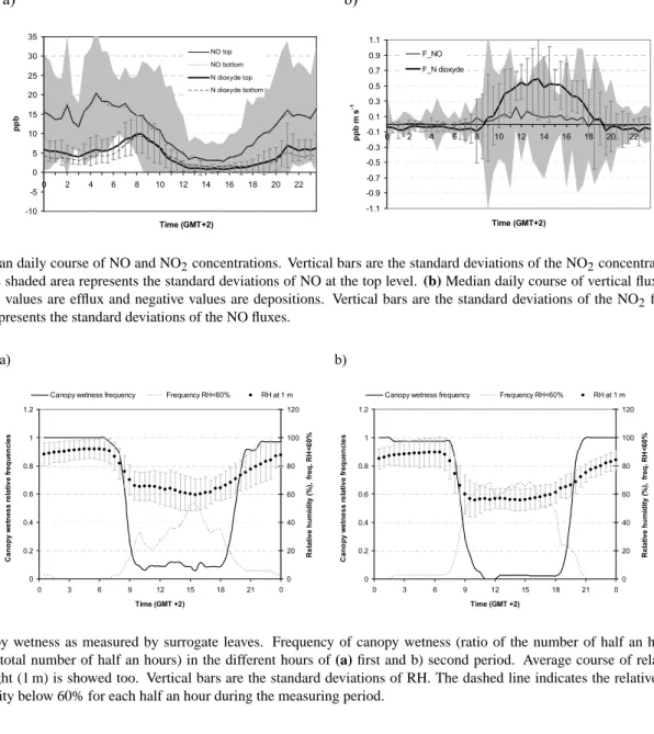
Mean nitric oxide (NO) concentrations remained fairly con-stant in the central hours of the day around a mean value of 3–4 ppb (Fig. 8a). Concentrations slowly increased during the night reaching a peak value of 20 ppb around 5 a.m., after which they decreased back to the typical diurnal values.
Nitrogen dioxide (NO2)concentrations remained around 1–2 ppb during the diurnal hours and rose to 6 ppb after sun-set. Similarly to NO, also NO2 concentrations showed a morning peak of 10 ppb which occurred between 8 and 9 a.m. Vertical fluxes of nitrogen oxides were considerably weaker than the already described ozone fluxes and were in general more variable. Nevertheless, the mean day trend
1 -2 0 2 4 6 8 10 12 14 5/5 12/5 19/5 26/5 2/6 9/6 16/6 23/6 30/6 7/7 14/7 21/7 28/7 Date E T [ m m H2 O m -2 ] , S W C [ % v o l ], R a in [ m m ] Rain ET SWC 30 SWC 60 SWC 100
Fig. 3. Daily averages of evapotranspiration, rain and soil water
content (v/v) during the whole measuring period. Soil water was measured at three different levels: 30 cm, 60 cm, 100 cm. Vertical dotted line is the separation between the two periods.
(Fig. 8b) reveals some regularities. During the measuring pe-riod NO showed a median positive flux (exiting the ecosys-tem) during the day (between 8 and 18 a.m.) and an almost null flux in the remaining night hours. The peak value of the median flux was about 0.2 ppb m s−1(±0.28 std. dev.)
On the contrary, the NO2 flux shows an almost constant median deposition rate around 0.06 ppb m s−1at night, with a weak peak of about 0.1 ppb m s−1 (±0.19) at 8 a.m. fol-lowed by an intense diurnal emission peak of 0.6 ppb m s−1 (±0.39 std. dev.) around 1 p.m.
The net NO efflux could be the result of soil emissions below the vegetation, while the efflux of NO2 may be in-terpreted as a photochemical effect. As refereed by Gao et al. (1993) and Monson and Holland (2001), NO concentra-tion show a steep decrease with height above the soil un-der a canopy, reaching a minimum near the middle of the canopy, while the O3induced oxidation of NO to O3within the canopy causes NO2 concentrations to be higher within the canopy than above resulting in a net efflux of NO2. The origin of such imbalance is not completely clear and could be attributed to advection, deposition and transforma-tion by nighttime chemistry of nitrogen species transported from Rome by the city plume.
4 Discussion
The order of magnitude of the ozone dose received by the maquis ecosystem is comparable to the dose received by the Holm Oak forest positioned just 0.8 km inland (Gerosa et al., 2009a) and it is also similar to the amount absorbed by bar-ley and wheat crops (Gerosa et al., 2003, 2004, 2005). Ap-parently, the dose does not vary greatly despite the evident structural differences of these ecosystems and the different leaf and canopy stomatal conductance. In all these cases, only a small portion of the ozone received by the ecosystem
1790 G. Gerosa et al.: Ozone, water and nitrogen fluxes in a maquis ecosystem 1 a) -100 0 100 200 300 400 500 600 700 0 3 6 9 12 15 18 21 0 Time (GMT +2) [W m -2] H LE Net Rad b) -100 0 100 200 300 400 500 600 700 0 3 6 9 12 15 18 21 0 Time (GMT +2) [W m -2] H LE Net Rad
Fig. 4. Energy fluxes: available energy (net-radiation), sensible heat and latent heat. Mean daily course in (a) the spring period and (b) the
summer period. Vertical bars are the standard deviations.
1 a) 0 1 2 3 4 5 6 7 8 9 0 6 12 18 0 Time (GMT +2) n m o l m -2 s -1
Sap flow derived EC, dry canopy EC, wet canopy
b) 0 1 2 3 4 5 6 7 8 9 0 6 12 18 0 Time (GMT +2) n m o l m -2 s -1
Sap flow derived EC, dry canopy EC, wet canopy
Fig. 5. Comparison of the ozone uptake (stomatal fluxes) obtained from the sap flow measurements and the eddy covariance (EC)
mea-surements in the late spring (a) and summer (b) periods. Graphs show averaged values of fluxes in each half an hour of the two distinct periods.
is effectively absorbed by the stomata. The greatest part of ozone, instead, is depleted in chemical-physical processes that altogether are termed non-stomatal deposition.
4.1 Stomatal uptake
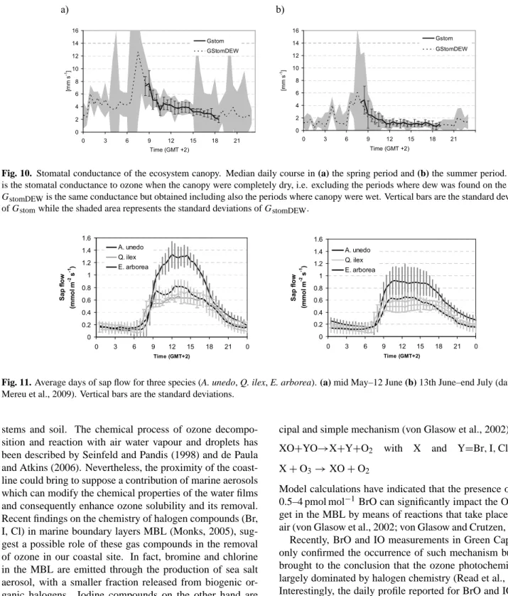
It is important to notice that night time hours are frequently characterized by thermal inversions, which determine the ac-cumulation of dew over the canopy and soil (Cieslik et al., 2009b; Mereu et al., 2009). The formation of dew during the night, as well as the drying of the leaf lamina and the evapo-ration early in the morning, are confirmed by the leaf wetness sensors (Fig. 9). The evaporation of water from the surfaces might lead to a misinterpretation of the data and to an over-estimation of the stomatal conductance. In Fig. 10 canopy stomatal conductance data are shown for both dry and wet canopy. Even if light intensity is sufficient to cue stomatal aperture already from the first hours of the morning (PPFD at 7 a.m. was around 300 µE m−2s−1)the early morning peak of stomatal conductance appears unrealistic. In fact, the sap
flux measurements performed on three species, (Mereu et al., 2009a) support this conclusion. With the only exception of the driest period (late July), sap flux showed a bell shaped trend and a peak in sap flux never occurred in the morning (Fig. 11). However, since the measured species only repre-sent 38% of the total cover (Fares et al., 2009) it could be ar-gued that the other species may be responsible for the morn-ing transpiration peak. But even this eventuality should be excluded by the fact that also two of the unmeasured species (P. latifolia, C. incanus) are known to behave in a similar way for the transpiration rate (Bombelli and Gratani, 2003). The only exception could be Rosmarinus officinalis (17% of the cover), but the SWC (9s<−1 MPa) was low enough to
ensure a reduction of its stomatal conductance of more than 80% (Clary et al., 2004). It is hence most likely that the ob-served morning peak is an artifact attributable simply to dew evaporation.
It is for this reason that the presented results were filtered in order to exclude fluxes measured when the canopy was wet and in the following hour. This underlines the importance of
1 a) 0 0.1 0.2 0.3 0.4 0.5 0.6 0.7 0.8 0.9 1 0 3 6 9 12 15 18 21 Time (GMT +2) Fstom/Ftot FStom/FcDEW b) 0 0.1 0.2 0.3 0.4 0.5 0.6 0.7 0.8 0.9 1 0 3 6 9 12 15 18 21 Time (GMT +2) Fstom/Ftot Fstom/FtotDEW
Fig. 6. Average stomatal fraction in the two periods (a) and (b). Fstom/Ftotis the ratio of the stomatal flux to the absolute value of total
deposition flux when the canopy were completely dry, i.e. excluding the periods where dew was found on the leaves; Fstom/FtotDEWis the same ratio but obtained including also the periods where canopy were wet. Vertical bars are the standard deviations referred to Fstom/Ftot while the shaded area represents the standard deviations of Fstom/FtotDEW.
verifying dry canopy conditions in EC based flux measure-ments, even in xeric environmeasure-ments, and the potential advan-tage of coupling EC measurements with sap flow gauges.
4.2 Non-stomatal deposition
The nature of the non-stomatal deposition (Fnstom), more than 50% percent in this study, is still not understood and different hypotheses have been made to explain it. Van Pul and Jacobs (1994), after observing that the Fnstomincreased with the efficiency of ozone transport inside the canopy, sug-gested the cause to be the destruction of ozone over the plant and soil surfaces, since they observed that the ozone transport efficiency is proportional to u∗and inversely related to the
Leaf Area Index (LAI) and to the vegetation height. Instead, in a laboratory experiment Rond´on (1993) showed that cutic-ular uptake by leaf waxes increased from a negligible rate at low levels of light intensity, to rates comparable with stom-atal uptake at light levels equivalent to strong sunlight con-ditions, thus suggesting an important role of solar radiation. Fowler et al. (2001) suggested that the relationship between
Fnstomand radiation reported by Rond´on (1993) and by Coe et al. (1995) could be explained as thermal decomposition of the ozone molecules intercepting the surfaces heated by radi-ation; they also estimated the energy of activation of this re-action to be 36 KJ mol−1. Kurpius and Goldstein (2003), in-stead, observed that the exponential form of the relationship between Fnstomand temperature was similar to the relation-ship between temperature and the emission rate of Volatile Organic Compounds (VOC). Based on this similarity, they advanced the hypothesis that a great fraction of the daytime ozone deposition could be a consequence of gas-phase re-actions with biogenic hydrocarbons and estimated that 45 to 55% of the total ozone flux could depend on such reac-tions. Loreto and Fares (2007) have shown the influence of monoterpenes on the removal of ozone both in the
bound-1 0 5000 10000 15000 20000 25000 1/5 11/5 21/5 31/5 10/6 20/6 30/6 10/7 20/7 30/7 date A O T 4 0 ( p p b h ) 0 5 10 15 20 25 S to m a ta l d o s e ( m m o l m -2 ) AOT40 at zm AOT40 at d+z0' AFst0 AFst1.6
Fig. 7. Evolution of Ozone exposure and stomatal dose during the
measuring period. The exposure is expressed as AOT40 calculated at measurement height and at momentum sink height (d+z0). The dose is expressed as cumulated stomatal flux AFst0, without any
flux threshold, and as AFst1.6 after the application of the
instanta-neous flux threshold of 1.6 nmol m−2s−1.
ary layer and inside the mesophyll, since the emission of monoterpenes was relevant at our site (Fares et al., 2009), monoterpenes reactions with ozone can play an important role in the non-stomatal deposition. However Mikkelsen et al. (2000) estimated from concurrently measured α- and β-pinene fluxes a maximum destruction potential of monoter-pene emissions corresponding only to 10% of the total ozone flux.
A role in non-stomatal ozone depletion has been also at-tributed to gas-phase tritration reactions with biogenic emis-sions of NO. The measurements of Dorsey et al. (2004) and of Pilegaard et al. (1999), and the precedent models of
1792 G. Gerosa et al.: Ozone, water and nitrogen fluxes in a maquis ecosystem 1 a) -10 -5 0 5 10 15 20 25 30 35 0 2 4 6 8 10 12 14 16 18 20 22 Time (GMT+2) p p b NO top NO bottom N dioxyde top N dioxyde bottom b) -1.1 -0.9 -0.7 -0.5 -0.3 -0.1 0.1 0.3 0.5 0.7 0.9 1.1 0 2 4 6 8 10 12 14 16 18 20 22 Time (GMT+2) p p b m s -1 F_NO F_N dioxyde
Fig. 8. (a) Mean daily course of NO and NO2concentrations. Vertical bars are the standard deviations of the NO2concentration at the top
level while the shaded area represents the standard deviations of NO at the top level. (b) Median daily course of vertical fluxes of NO and NO2. Positive values are efflux and negative values are depositions. Vertical bars are the standard deviations of the NO2fluxes, and the shaded area represents the standard deviations of the NO fluxes.
1 a) 0 0.2 0.4 0.6 0.8 1 1.2 0 3 6 9 12 15 18 21 0 Time (GMT +2) C a n o p y w e tn e s s r e la ti v e f re q u e n c ie s 0 20 40 60 80 100 120 R e la ti v e h u m id it y ( % ), fr e q . R H < 6 0 %
Canopy wetness frequency Frequency RH<60% RH at 1 m
b) 0 0.2 0.4 0.6 0.8 1 1.2 0 3 6 9 12 15 18 21 0 Time (GMT +2) C a n o p y w e tn e s s r e la ti v e f re q u e n c ie s 0 20 40 60 80 100 120 R e la ti v e h u m id it y ( % ), fr e q . R H < 6 0 %
Canopy wetness frequency Frequency RH<60% RH at 1 m
Fig. 9. Canopy wetness as measured by surrogate leaves. Frequency of canopy wetness (ratio of the number of half an hours with wet
canopy to the total number of half an hours) in the different hours of (a) first and b) second period. Average course of relative humidity at canopy height (1 m) is showed too. Vertical bars are the standard deviations of RH. The dashed line indicates the relative frequency of relative humidity below 60% for each half an hour during the measuring period.
Duyzer et al. (1995) and Walton et al. (1997), highlighted that NO emissions from forest soils not only affect the mag-nitude and the direction of the NO2fluxes, but also the inten-sity of ozone fluxes. Nevertheless, the influence on the latter is usually weak, but not negligible, and can become relevant in case of a high soil NO efflux (Pilegaard et al., 1999), when a substantial (∼30%) amount of the total ozone flux could be accounted for by chemical reactions, especially at night (Pilegaard, 2001; Walton et al., 1997). Finally, Altimir et al. (2004) found an influence of the atmospheric humidity on non-stomatal deposition at night., with an hyperbolic in-crease of surface conductance to ozone with saturating RH %.
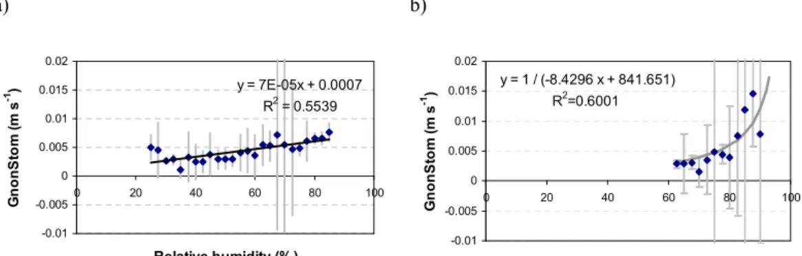
In this study, the analysis of the data presented in Figs. 12 and 13 allows to support only the hypothesis of a direct influ-ence of atmospheric humidity on non-stomatal deposition. A
gas-phase reaction with NO of biogenic and antropic origin could be observed but only at high efflux rates as reported by Pilegaard et al. (1999).
The occurrence of this reaction is revealed by the hyper-bolic dependence (R2=0.95) of Fnstom on the NO2 fluxes observed over the canopy (Fig. 12f).
The dependence on RH, instead, is revealed by the me-dian values of non-stomatal conductance, that, increased lin-early together with the absolute humidity of air (R2=0.63) and the relative humidity (R2=0.55) when the canopy was completely dry (Figs. 12d and 13a). When the canopy was wet (mostly at night in our site) the relationship became hy-perbolic (R2=0.60) (Fig. 13b) as already found by Altimir et al. (2004). In this last case, ozone is not only removed by reactions with atmospheric water, but also dissolved in the water film deposited over the colder surfaces, i.e. leaves,
1 a) 0 2 4 6 8 10 12 14 16 0 3 6 9 12 15 18 21 Time (GMT +2) [m m s -1] Gstom GStomDEW b) 0 2 4 6 8 10 12 14 16 0 3 6 9 12 15 18 21 Time (GMT +2) [m m s -1] Gstom GStomDEW
Fig. 10. Stomatal conductance of the ecosystem canopy. Median daily course in (a) the spring period and (b) the summer period. Gstom
is the stomatal conductance to ozone when the canopy were completely dry, i.e. excluding the periods where dew was found on the leaves;
GstomDEWis the same conductance but obtained including also the periods where canopy were wet. Vertical bars are the standard deviations of Gstomwhile the shaded area represents the standard deviations of GstomDEW.
0 0.2 0.4 0.6 0.8 1 1.2 1.4 1.6 0 3 6 9 12 15 18 21 0 Time (GMT+2) S a p f lo w (m m o l m -2 s -1) A. unedo Q. ilex E. arborea 0 0.2 0.4 0.6 0.8 1 1.2 1.4 1.6 0 3 6 9 12 15 18 21 0 Time (GMT+2) S a p f lo w ( m m o l m -2 s -1) A. unedo Q. ilex E. arborea
Fig. 11. Average days of sap flow for three species (A. unedo, Q. ilex, E. arborea). (a) mid May–12 June (b) 13th June–end July (data from
Mereu et al., 2009). Vertical bars are the standard deviations.
stems and soil. The chemical process of ozone decompo-sition and reaction with air water vapour and droplets has been described by Seinfeld and Pandis (1998) and de Paula and Atkins (2006). Nevertheless, the proximity of the coast-line could bring to suppose a contribution of marine aerosols which can modify the chemical properties of the water films and consequently enhance ozone solubility and its removal. Recent findings on the chemistry of halogen compounds (Br, I, Cl) in marine boundary layers MBL (Monks, 2005), sug-gest a possible role of these gas compounds in the removal of ozone in our coastal site. In fact, bromine and chlorine in the MBL are emitted through the production of sea salt aerosol, with a smaller fraction released from biogenic or-ganic halogens. Iodine compounds on the other hand are largely released as organic compounds and molecular iodine from micro and macro algae that accumulate iodine from the sea water (von Glasow, 2008). Chemical and photochemi-cal reactions rapidly convert these compounds in halogenated monoxides (Monks, 2005). These latter compounds are di-rectly responsible for the catalytic removal through one
prin-cipal and simple mechanism (von Glasow et al., 2002): XO+YO→X+Y+O2 with X and Y=Br, I, Cl (11)
X + O3→XO + O2 (12)
Model calculations have indicated that the presence of only 0.5–4 pmol mol−1BrO can significantly impact the O3 bud-get in the MBL by means of reactions that take place in the air (von Glasow et al., 2002; von Glasow and Crutzen, 2004). Recently, BrO and IO measurements in Green Cape, not only confirmed the occurrence of such mechanism but also brought to the conclusion that the ozone photochemistry is largely dominated by halogen chemistry (Read et al., 2008). Interestingly, the daily profile reported for BrO and IO con-centrations is similar to the ozone deposition found in this study. Concentrations of both gasses reach a maximum around 10 a.m., remain constant until 14 p.m. for IO and until 7 p.m. for BrO, and decrease to 0 afterwards. In the coastal site subject to a considerable external source of NOxat night, as in this case, the formation of halogenated nitrates- as BrONO2- can take place. At sunrise, these compounds pho-tolyse freeing NO2and halogenated oxides that may trigger
1794 G. Gerosa et al.: Ozone, water and nitrogen fluxes in a maquis ecosystem 1 a) y = -0.0019x + 0.0056 R2 = 0.126 -0.01 -0.005 0 0.005 0.01 0.015 0.02 0 0.2 0.4 0.6 0.8 1 u* (m/s) G n o n S to m ( m s -1 ) b) y = -1E-05x + 0.0049 R2 = 0.0004 -0.01 -0.005 0 0.005 0.01 0.015 0.02 15 20 25 30 35 T (°C) G n o n S to m ( m s -1 ) c) y = 5E-07x + 0.0037 R2 = 0.1001 -0.01 -0.005 0 0.005 0.01 0.015 0.02 0 500 1000 1500 2000 PPFD (µµµµmol m-2 s-1) G n o n s to m ( m s -1 ) d) y = 0.0003x + 0.0002 R2 = 0.6266 -0.01 -0.005 0 0.005 0.01 0.015 0.02 0 5 10 15 20 25 χ χχ χ (g m-3) G n o n S to m ( m s -1 ) e) y = 3E-05x + 0.0044 R2 = 0.0003 -0.01 -0.005 0 0.005 0.01 0.015 0.02 -1 -0.5 0 0.5 1 F_NO (ppb m/s) G n o n S to m ( m s -1 ) f) -0.02 0 0.02 0.04 0.06 0.08 -0.5 0 0.5 1 F_NO2 (ppb m/s) G n o n S to m ( m s -1 ) y = 1 / (-287.2 x + 303.7) R2=0.95648
Fig. 12. Non-stomatal deposition (GnonStom)versus air turbulence (u∗), air temperature (T ), solar radiation (PPFD) and absolute air humidity
(χ ), NO and NO2fluxes (F NO and F NO2). Points are median values of non-stomatal conductance for each bin of the variable in x-axis and vertical bars represent standard deviations. Note than the y-axis in the F NO2graph has a different scale. Positive flux values indicate efflux and negative values depositions. Data from the whole measuring period have been considered.
and amplify the catalytic destruction of ozone. Such a pro-cess is what is suggested by the so-called “sunrise ozone de-struction” reported by different authors (Nagao et al., 1999; Galbally et al., 2000; Watanabe et al., 2005). Such a morn-ing peak of ozone depletion was already reported for a close site (Gerosa et al., 2005, 2009) and it occurred again during this campaign. The morning peak, especially in the first pe-riod, can be inferred from Figs. 2 and 6, where a rise in total ozone deposition is not supported by a concomitant rise in ozone stomatal uptake. This hypothesis would also explain the NO2efflux in excess observed in the maquis during the
day. In fact, the air masses of the city plume rich in nitrate species, would first be transported offshore from the night breeze and return to land during the day under the form of organic and halogenated nitrous compounds. Hence, if the hypothesis of the role of the chemistry of halogenated com-pounds should be confirmed also for this site, the correla-tion found with humidity could simply be an indicator of the transport of halogenated species from the sea when the wind was blowing from offshore.
1 a) y = 7E-05x + 0.0007 R2 = 0.5539 -0.01 -0.005 0 0.005 0.01 0.015 0.02 0 20 40 60 80 100 Relative humidity (% ) G n o n S to m ( m s -1) b) -0.01 -0.005 0 0.005 0.01 0.015 0.02 0 20 40 60 80 100 Relative humidity (% ) G n o n S to m ( m s -1 ) y = 1 / (-8.4296 x + 841.651) R2=0.6001 .
Fig. 13. Non-stomatal deposition and relative air humidity in (a) dry canopy and (b) wet canopy conditions. Vertical bars are the standard
deviations. Data from the whole measuring period have been considered.
4.3 Ozone risk assessment
Ozone exposure was calculated as AOT40 using ozone con-centrations both at the measuring point and at canopy level, calculating the latter ones by means of the DDIM.
In both cases the ozone exposure exceeded the critical level (CL) of 5000 ppb h established for plants protection, re-vealing a potentially ozone hazard condition for the maquis ecosystem. Considering that the vegetative period of maquis is much longer than our measuring period, it can be reason-ably supposed that the exposure to which these ecosystems are usually subject to is very high.
It is worth noticing that the CL was exceeded very soon by the AOT40 evaluated at the measuring height (23 May), and only one month and half later (5 July) at the canopy height
d+z0. The two metrics gave very different results, highlight-ing the importance of followhighlight-ing the indications of the Map-ping Manual (ICP Modelling and MapMap-ping, 2004), the dis-respect of which may bring to considerable overestimation of the risks – a three fold higher in this case – and to erro-neous conclusions. The risk of overestimating the negative effects of ozone on the vegetation is particularly high in the Mediterranean area, where the concentrations of this pollu-tant are usually high (Paoletti, 2006).
The failure to estimate ozone concentrations at top canopy height is not necessarily due to negligence, but to the lack of the necessary information to infer the ozone gradient above the canopy when using data from monitoring network sta-tions, which usually sample at a height of 3 m. The deter-mination of such gradient, in fact, requires knowledge of the aerodynamic state of the atmospheric surface layer (turbu-lence/stability) and the conductance to ozone of the ecosys-tem, which is known to vary rapidly as a response to the en-vironmental conditions and to the physiological state of the plant. Ultimately, ozone exposure at top canopy height can be determined only through direct flux measurements. Mea-surements that, as in this case, can be more profitably used to determine the stomatal ozone uptake, one of the most
sig-nificant toxicological parameters. However, it must be no-ticed that the phytotoxical part of ozone taken up by plants could be reduced by meshopyll reactions between ozone and monoterpens; quantification of the detoxification process has still some uncertainties but this process could explain the high resistance of Mediterranean species to the ozone.
The dose of ozone absorbed by the vegetation during the measuring period, appears well above the provisional critical flux level of 4 mmol m−2, expressed as AF
st1.6, for the
re-duction of 5% of biomass growing in beech and birch (ICP Modelling and Mapping, 2004; Karlsson et al., 2004)
This dose, however, is below the critical dose for the appearance of visible injury symptoms on leaves (30 mmol m−2) of beech and poplar found in recent OTC ex-periments (Gerosa et al., 2009b). These exex-periments reported also that even at lower doses, even asymptomatic species such as Q. robur, when exposed to ozone, showed a marked reduction in the photosynthetic efficiency over a long period (Bussotti et al., 2007). Hence, even if direct assimilation measurements by Fares et al. (2009) in the first measuring period did not show an assimilation reduction and no leaf injuries were observed in this study, it cannot be a priori ex-cluded that photosynthetic assimilation was negatively influ-enced by ozone over the whole measuring period (5 June to 31 July 2007) and ozone activated antioxidant systems capa-ble of protecting the vegetation from photo-oxidative stress (Nali et al., 2004; Paoletti, 2006).
In any case, in a multi specific ecosystem the ozone risk assessment might to be more precise and take into account the specific physiology of each species. Some species, in fact, can largely account for the dose of ozone absorbed by the ecosystem and hence may be relatively more affected by this pollutant and trigger future changes in ecosystem composition. This is what happened, for example, for the three species A. unedo, Q. ilex, E. arborea considered in the Fig. 11, which shows different values of stomatal conduc-tance for each species and hence each one absorbed a differ-ent ozone dose.
1796 G. Gerosa et al.: Ozone, water and nitrogen fluxes in a maquis ecosystem
Finally, the measured dose is very close to the 24 mmol m−2estimated for forests, in the same area and for the year 2000, by the renovated deposition module DO3 SE-EMEP (Simpson et al., 2007). But it should be noted that the model estimation covered 6 months of the entire growing season and not only the central three months, as in our case.
In any case model parameterizations for this ecosystem are still necessary.
5 Conclusions
The maquis ecosystem acted as a net sink for ozone and the ozone deposition was quite high. Nevertheless, only a minor part of the ozone flux (32.8%) was absorbed by vegetation through the stomata. The stomatal uptake was influenced by water availability and decreased throughout the measuring period as the season became dryer.
The remaining part of the ozone deposition, the so called non-stomatal one, was positively influenced by air humidity and by nitrogen oxides. Nevertheless the influence of these latter was weak, and was evident only when nitrogen fluxes were particularly high. No influence with other measured factors, such as temperature, solar radiation and turbulence intensity were found. Moreover, due to the coastal loca-tion of the measuring site, a possible role on ozone deple-tion of halogenated species advected from the sea was also suggested as a working hypothesis, even if it should be con-firmed by new measurements.
The maquis ecosystem resulted at high risk for ozone con-sidering both AOT40 and AFst1.6 approaches, just on a three
months base instead of six months as suggested by UN-ECE. Hence, negative effects on the vegetation community cannot be excluded for this particular ecosystem, and more in gen-eral for the Mediterranean maquis ecosystems. However the different behaviors shown by the exposure and the dose met-rics highlighted the need for field measurements in order to realize a better risk assessment.
Finally a significant dataset is now available in ASCII for-mat for testing, refining and validating deposition models on this type of ecosystems and Mediterranean climatic condi-tions.
Acknowledgements. The field campaign was supported by the
VOCBAS and ACCENT/BIAFLUX programs. We’re also grate-ful to the Exchange of Staff funding Program of the AC-CENT/BIAFLUX Network of Excellence for its support.
A special thank to the Scientific Committee of the Presidential Estate of Castelporziano and to its staff who allowed this work. Edited by: F. Loreto
References
Altimir, N., Tuovinen, J., Vesala, T., Kulmala, M., and Hari, P.: Measurements of ozone removal by Scots pine shoots:
calibra-tion of a stomatal uptake model including the non-stomatal com-ponent, Atmos. Environ., 38, 2387–2398, 2004.
Altimir, N., Kolari, P., Tuovinen, J.-P., Vesala, T., B¨ack, J., Suni, T., Kulmala, M., and Hari, P.: Foliage surface ozone deposition: a role for surface moisture?, Biogeosciences, 3, 209–228, 2006, http://www.biogeosciences.net/3/209/2006/.
Ashmore, M., B¨uker, P., Emberson, L., Terry, A. C., and Toet, S.: Modelling stomatal ozone flux and deposition to grassland com-munities across Europe, Environ. Pollut., 146, 659–670, 2007. Benton, J., Fuhrer, J., Gimeno, B. S., Sk¨arby, L., Palmer-Brown,
D., Ball, G. R., Roadknight, C., and Mills, G.: An international cooperative programme indicates the widespread occurrence of ozone injury on crops, Agric., Ecosyst. Env., 78, 19–30, 2000. Bermejo, V., Gimeno, B. S., Sanz, M. J., De La Torre, D., and Gil,
J. M.: Assessment of the ozone sensitivity of 22 native plant species from Mediterranean annual pastures based on visible in-jury, Atmos. Environ., 37, 4667–4677, 2003.
Bombelli, A. and Gratani, L.: Interspecific Differences of Leaf Gas Exchange and Water Relations of Three Evergreen Mediter-ranean Shrub Species, Photosynthetica, 41, 619–625, 2003. Bussotti, F. and Gerosa, G.: Are the Mediterranean forests in
South-ern Europe threatened from ozone?, J. Medit. Ecol., 3, 23–34, 2002.
Bussotti, F., Cozzi, A., and Ferretti, M.: Field Surveys of Ozone Symptoms on Spontaneous Vegetation. Limitations and Poten-tialities of the European programme, Environ. Monit. Assess., 115, 335–348, 2006.
Bussotti, F., Desotgiu, R., Cascio, C., Strasser, R. J., Gerosa, G., and Marzuoli, R.: Photosynthesis responses to ozone in young trees of three species with different sensitivities, in a 2-year open-top chamber experiment (Curno, Italy), Physiologia Plant., 130, 122–135, 2007.
Cieslik, S.: Ozone fluxes over various plant ecosystems in Italy: A review, Environ. Pollut., 157, 1487–1496, 2009a
Cieslik, S. A., Gerosa, G., Finco, A., Matteucci, G., Cape, N., and Misztal, P.: Turbulence in a coastal Mediterranean area: surface fluxes and related parameters at Castel Porziano, Italy, Biogeo-sciences Discuss., 6, 3355–3372, 2009b,
http://www.biogeosciences-discuss.net/6/3355/2009/.
Clary, J., Save, R., Biel, C., and Herralde, F.: Water relations in competitive interactions of Mediterranean grasses and shrubs, Ann. Appl. Biol., 144, 149–155, 2004.
Coe, H., Gallagher, M., Choularton, T., and Dore, C.: Canopy scale measurements of stomatal and cuticular O∼3 uptake by Sitka Spruce, Atmos. Environ., 29, 1413–1413, 1995.
De Paula, J. and Atkins, P.: Explorations in Physical Chemistry, Oxford University Press, 2006.
Dorsey, J. R., Duyzer, J. H., Gallagher, M. W., Coe, H., Pilegaard, K., Weststrate, J. H., Jensen, N. O., and Walton, S.: Oxidized nitrogen and ozone interaction with forests. I: Experimental ob-servations and analysis of exchange with Douglas fir, Q. J. Roy. Meteor. Soc., 130, 1941–1955, 2004.
Dutaur, L., Carrara, S., and Lopez, A.: The detection of nonsta-tionarity in the determination of deposition fluxes, Proceedings of EUROTRAC Symposium’98, 171–176, 1999.
Duyzer, J., Weststrate, H., and Walton, S.: Exchange of ozone and nitrogen oxides between the atmosphere and coniferous forest, Water, Air, Soil Pollut., 85, 2065–2070, 1995.
Fay, J. A. and Hoult, D. P.: Akademija Nauk CCCP, Leningrad,
Trudy Geofizicheskowo Instituta, 151(24), 163–187, 1954. Elvira, S., Bermejo, V., Manrique, E., and Gimeno, B. S.: On the
response of two populations of Quercus coccifera to ozone and its relationship with ozone uptake, Atmos. Environ., 38, 2305– 2311, 2004.
Emberson, L. D., Massman, W. J., B¨uker, P., Soja, G., van de Sand, I., Mills, G., and Jacobs, C.: The development, evaluation and application of O3flux and flux-response models for additional agricultural crops, Critical Levels for Ozone: Further Apply-ing and DevelopApply-ing the Flux-based Concept, Innsbruck, Austria, 2005.
Emberson, L., B¨uker, P., and Ashmore, M.: Assessing the risk caused by ground level ozone to European forest trees: A case study in pine, beech and oak across different climate regions, Environ. Pollut., 147, 454–466, 2007.
Fares, S., Mereu, S., Scarascia Mugnozza, G., Vitale, M., Manes, F., Frattoni, M., Ciccioli, P., Gerosa, G., and Loreto, F.: The ACCENT-VOCBAS field campaign on biosphere-atmosphere interactions in a Mediterranean ecosystem of Castelporziano (Rome): site characteristics, climatic and meteorological con-ditions, and eco-physiology of vegetation, Biogeosciences, 6, 1043–1058, 2009,
http://www.biogeosciences.net/6/1043/2009/.
Felzer, B., Kicklighter, D., Melillo, J., Wang, C., Zhuang, Q., and Prinn, R.: Effects of ozone on net primary production and carbon sequestration in the conterminous United States using a biogeo-chemistry model, Tellus B, 56, 230–248, 2004.
Foken, T.: Micrometeorology, Springer-Verlag, Berlin Heidelberg, ISBN: 978-3-540-74665-2, 308 pp., 2008.
Fowler, D., Flechard, C., Cape, J. N., Storeton-West, R. L., and Coyle, M.: Measurements of Ozone Deposition to Vegetation Quantifying the Flux, the Stomatal and Non-Stomatal Compo-nents, Water, Air, Soil Pollut., 130, 63–74, 2001.
Galbally, I. E., Bentley, S. T., and Meyer, C. P. M.: Mid-latitude marine boundary-layer ozone destruction at visible sunrise ob-served at Cape Grim, Tasmania, 41 S, Geophys. Res. Lett, 27, 3841–3844, 2000.
Gao, W., Wesely, M., and Doskey, P.: Numerical modeling of the turbulent diffusion and chemistry of NOx, O3, isoprene, and other reactive trace gases in and above a forest canopy, J. Geo-phys. Res., 98, 18339–18354, 1993.
Gerosa, G., Cieslik, S., and Ballarin-Denti, A.: Micrometeorolog-ical determination of time-integrated stomatal ozone fluxes over wheat: a case study in Northern Italy, Atmos. Environ., 37, 777– 788, 2003.
Gerosa, G., Finco, A., Mereu, S., Vitale, M., Manes, F., and Ballarin Denti, A.: Comparison of seasonal variations of ozone exposure and fluxes in a Mediterranean Holm oak forest between the ex-ceptionally dry 2003 and the following year, Environ. Pollut., 157, 1737–1744, 2009a.
Gerosa, G., Marzuoli, R., Cieslik, S., and Ballarin-Denti, A.: Stom-atal ozone fluxes over a barley field in Italy.“Effective exposure” as a possible link between exposure-and flux-based approaches, Atmos. Environ., 38, 2421–2432, 2004.
Gerosa, G., Marzuoli, R., Desotgiu, R., Bussotti, F., and Ballarin-Denti, A,: Validation of the stomatal flux approach for the assess-ment of ozone effects on young forest trees, A summary report of the TOP (Transboundary Ozone Pollution) experiment at Curno, Italy. Environ. Pollut., 157, 1497–1505, 2009b
Gerosa, G., Vitale, M., Finco, A., Manes, F., Ballarin-Denti, A., and Cieslik, S. A.: Ozone uptake by an evergreen Mediterranean Forest (Quercus ilex) in Italy, Part I: Micrometeorological ?ux measurements and ?ux partitioning, Atmos. Environ., 39, 3255– 3266, 2005.
Gr¨unhage, L., Haenel, H., and J¨ager, H.: The exchange of ozone between vegetation and atmosphere: micrometeorological mea-surement techniques and models, Environ. Pollut., 109, 373–392, 2000.
Hicks, B. B. and Matt, D. R.: Combining biology, chemistry, and meteorology in modeling and measuring dry deposition, J. At-mos. Chem., 6, 117–131, 1988.
Hicks, B., Baldocchi, D., Meyers, T., Hosker, R., and Matt, D.: A preliminary multiple resistance routine for deriving dry deposi-tion velocities from measured quantities, Water, Air, Soil Pollut., 36, 311–330, 1987.
ICP Modelling and Mapping.: Manual on Methodologies and Cri-teria for Modelling and Mapping Critical Loads and Levels and Air Pollution Effects, Risks and Trends. Federal Environmental Agency (Umweltbundesamt),Berlin. UBA-Texte52/04, available from: www.icpmapping.org, 2004.
Kaimal, J. and Finnigan, J.: Atmospheric Boundary Layer Flows: Their Structure and Measurement, Oxford University Press, USA, 1994.
Karlsson, P. E., Braun, S., Broadmeadow, M., Elvira, S., Emberson, L., Gimeno, B., Thiec, D. L., Novak, K., Oksanen, E., Schaub, M., Uddling, J., and Wilkinson, M.: Risk assessments for forest trees: The performance of the ozone flux versus the AOT con-cepts, Environ. Pollut., 146, 608–616, 2007.
Karlsson, P., Uddling, J., Braun, S., Broadmeadow, M., Elvira, S., Gimeno, B., Le Thiec, D., Oksanen, E., Vandermeiren, K., and Wilkinson, M.: New critical levels for ozone effects on young trees based on AOT40 and simulated cumulative leaf uptake of ozone, Atmos. Environ., 38, 2283–2294, 2004.
Keronen, P., Reissell, A., Rannik, U., Pohja, T., Siivola, E., Hiltunen, V., Hari, P., Kulmala, M., and Vesala, T.: Ozone flux measurements over a Scots pine forest using eddy covari-ance method: performcovari-ance evaluation and comparison with flux-profile method, Boreal Env. Res., 8, 425–444, 2003.
King, J. S., Kubiske, M. E., Pregitzer, K. S., Hendrey, G. R., Mc-Donald, E. P., Giardina, C. P., Quinn, V. S., and Karnosky, D. F.: Tropospheric O3 compromises net primary production in young stands of trembling aspen, paper birch and sugar maple in re-sponse to elevated atmospheric CO2, New Phytologist, 168, 623– 636, 2005.
Kurpius, M. and Goldstein, A.: Gas-phase chemistry dominates O3 loss to a forest, implying a source of aerosols and hy-droxyl radicals to the atmosphere, Geophys. Res. Lett., 30, 1371, doi:10.1029/2002GL016785, 2003.
Loreto, F. and Fares, S.,: Is ozone flux inside leaves only a damage indicator? Clues from volatile isoprenoid studies, Plant Physiol., 143, 1096–1100, 2007.
Marzuoli, R., Gerosa, G., Desotgiu, R., Bussotti, F., and Ballarin-Denti, A.: Ozone fluxes and foliar injury development in the ozone-sensitive poplar clone Oxford (Populus maximowiczii x Populus berolinensis): a dose–response analysis, Tree Physiol., 29(1), 67–76, doi:10.1093/treephys/tpn012, 2008.
Massman, W.J.: A review of the molecular diffusivities of H2O, CO2, CH4, CO, O3, SO2, NH3, N2O, NO, and NO2in air, O2