Mesophotic red coral population: genetic variability and connectivity

ALMA MATER STUDIORUM

UNIVERSITA' DI BOLOGNA

FACOLTA' DI SCIENZE MATEMATICHE , FISICHE E NATURALI

Corso di laurea magistrale in Biologia Marina

MESOPHOTIC RED CORAL POPULATIONS:

GENETIC VARIABILITY AND CONNECTIVITY

Relatore: Presentata da:

Prof. Marco Abbiati Rosa Angela Pugliese

Correlatore:

Dott.ssa Federica Costantini

II sessione

Anno Accademico 2011/2012

INDEX

ABSTRACT

1. INTRODUCTION

1.1 POPULATION GENETICS AND MOLECULAR ECOLOGY APPROACHES………1

1.2 MESOPHOTIC CORAL ECOSYSTEM - MCE ………3

1.3 MEDITERRANEAN MESOPHOTIC HABITATS……….5

2. Corallium rubrum

2.2 BIOLOGY AND REPRODUCTION………...…..11

2.3 HARVESTING PRESSURE AND NATURAL MORTALITY ………..14

2.4 POPULATION GENETICS………..……...17

3. MATERIALS AND METHODS

3.2 DNA EXTRACTION AND MOLECULAR ANALYSIS……….……….22

3.3 MICROSATELLITE MARKERS 3.3.1 Genetic Variability...23

3.3.2 Population genetic differentiation………...……24

3.4 MITOCHONDRIAL MARKERS 3.4.1 Genetic variability……….…………...………...25

3.4.2 Population genetic differentiation………...……26

4. RESULTS

4.1.1 Genetic Variability………..………...27

4.1.2 Population genetic differentiation...………...29

4.2 MITOCHONDRIAL MARKERS 4.2.1 Sequence variation………...………..34

4.2.2 Genetic differentiation between populations………..………...36

5. DISCUSSION

5.1

5.2 GENETIC DIFFERENTIATION...42

6. CONCLUSION

ABSTRACT

The Mediterranean red coral (Corallium rubrum, L. 1758) is a long living octocoral that has been commercially harvested since ancient time for its red axial calcitic skeleton. At present, shallow-water red coral populations are overexploited and consequently in decline, so deeper populations below 50m (mesophotic populations) have currently become the most commercially harvested. Unfortunately, very little is known about the biology and ecology of these mesophotic populations and for their management and conservation a better understanding of their genetic structuring and connectivity is needed. The present study was carried out to define genetic variability and structuring in Corallium rubrum populations located between 60 and 120 metres depth, collected in three different areas of the Tyrrhenian Sea (Liguria, Toscana and Campania). A total of fourteen populations were sampled and analyzed by means of a set of 10 nuclear microsatellite loci and the putative control region of the mitochondrial DNA (MtC). Microsatellite genotyping indicated that all loci were polymorphic and showed significant deviations from Hardy–Weinberg equilibrium, due to an heterozygote deficiency, probably related to the presence of null alleles and/or inbreeding, as was previously observed in shallow-water populations. Both types of molecular markers showed high genetic similarity between Liguria and Toscana populations (Northern Tyrrhenian) compared to Campania populations (Southern Tyrrhenian). The genetic differentiation observed between North and South Tyrrhenian populations follows a weak but significant pattern of isolation by distance. However, low correlation between genetic divergence and geographic distances detected using the mitochondrial marker suggests that observed patterns could also be partially related to the presence of a long term barrier to gene flow, given the hydrodynamic and geological characteristic of the studied area. At smaller spatial scales (within areas) the two molecular markers indicate different structures, probably due to the low polymorphism of MtC or to the occurrence of some historical links within regions. These results show that mesophotic red coral populations are mainly self recruiting, similarly to the shallow water ones, with a limited effective dispersal ability of the larvae, further enhanced by the patchy distribution of suitable habitats. According to our results, management strategies of red coral harvesting in the mesophotic habitats should be defined at a regional level, being highly advisable the creation of deep-sea marine protected areas, in order to maximise the genetic diversity of this highly vulnerable populations of red coral in this unique habitats.

1

1.INTRODUCTION

1.1 Population genetics and molecular ecology approaches

Molecular ecology is the discipline that applies population genetics, phylogenetic, and more recently genomics to traditional ecological questions, e.g., species diagnosis, conservation and assessment of biodiversity, or species-area relationships (Moritz 2002).

Population genetics is a field of biology that studies genetic composition, populations structure, and the changes in genetic variability that result from the interaction of various evolutionary processes. Genetic variability within and between populations, can be assessed by studying the processes influencing the allelic and genotypic frequencies of one or more gene loci. These processes include mutation (the original multi-level source of genetic variation in a population), genetic drift (casual changes in allele frequencies caused by small population size), gene flow (movement between groups that results in genetic exchange), natural selection, and inbreeding (Hedrick 2009). A population or a species that, for any reason, loses part of its gene pool runs into a higher risk of extinction, losing part of its potential adaptability to new environmental conditions (Saccheri et al. 1998; Hughes et al. 2008). In populations of small size, such as in overexploited species, increase of genetic drift and inbreeding leads to an increase of homozygosity which in turn leads to reduction in fitness, defined as an “inbreeding depression” (Newman et al. 1997). In this context dispersive capacity and connectivity between populations, are the key elements to ensure population resilience after a disturbance (Palumbi 2004). Connectivity, in sessile marine species such as corals, is closely associated with dispersal larval capacity, besides the presence of physico-chemical barriers (hydrodynamics, geomorphology, thermal gradients, and lack of suitable habitats for colonization). In coral populations, given the difficulties associated with direct observations of the larval dispersal process, the difficulties in accessibility to populations, an important part of the estimation of their effective larval dispersal capacity may come from molecular data (Moritz & Lavery 1996).

Genetic diversity and connectivity can be measured using various DNA-based methods and other techniques. Nowadays three important components have come together: efficient techniques to examine informative segments of DNA, statistics to analyse DNA data and the availability of easy-to-use computer packages. Genetic

2

markers such as allozymes, microsatellites and mitochondrial and nuclear DNA sequences can be used to estimate many parameters of interest to ecologists, such as migration rates, population size, bottlenecks, kinship and more (Avise 2004). Based on evolutionary rate of the markers, different genes are chosen to perform different investigations at different taxonomic levels: genes with a low rate of mutation are suitable for interspecific studies (e.g. phylogeny at high taxonomic levels), while genes with high mutation rate are used for intraspecific studies (e.g. population genetics studies). In the phylum Cnidaria mitochondrial DNA, due its low evolutionary rate, is not suitable for the study of population genetics (Costantini et al. 2003, McFadden et al. 2006, Shearer et al. 2002, Hellberg 2006): Nuclear microsatellite loci, tandem repeats of 2-10 base pairs, revealed a high genetic variability. High levels of polymorphism support microsatellites being one of the most useful markers for intraspecific studieson genetic variation. Microsatellites have the potential to provide estimates of migration, to distinguish high rates of migration from panmixia, and to allow estimates of the relatedness among individuals. Several recent reviews detail the variety of molecular techniques now available, and the ecological questions that they can address (Bossart & Prowell 1998; Davies et al. 1999; Luikart & England 1999; Sunnucks 2000; Manel et al. 2003, 2005; Beaumont & Rannala 2004).

Molecular markers allow identifying populations of organisms at risk, or threatened of extinction. These populations are often described as stocks or ESU (Evolutionarily Significant Units). The identification of these units is difficult but important to determine which populations should be subject to legislative interventions and action plans for their conservation, management and sustainable use.

3

1.2 Mesophotic coral ecosystem- MCE

In the past decades, human induced disturbance (e.g. habitat loss and fragmentation, global climate change, overexploitation and other effects due to fishing, pollution and tourism) has increased in marine shallow habitats (Ballesteros 2006; Airoldi & Beck 2007).

With the decline of shallow coastal water resources, due to increasing demands and development of new technologies; human activities, most notably fishing, have expanded offshore and into deeper waters (Morato et al. 2006) Moreover, in the last years, researchers have shown that the deep-sea is more sensitive to human and natural impacts than previously thought (Davies et al. 2007) and that the same threats faced by shallow water species can act directly or indirectly on deep species affecting their distribution, population dynamics, growth and genetic structure (Smith et al. 2010; Bongaerts et al 2010). Therefore, conservation and sustainable management of marine resources in deep-sea ecosystems has become a binding priority for marine scientists.

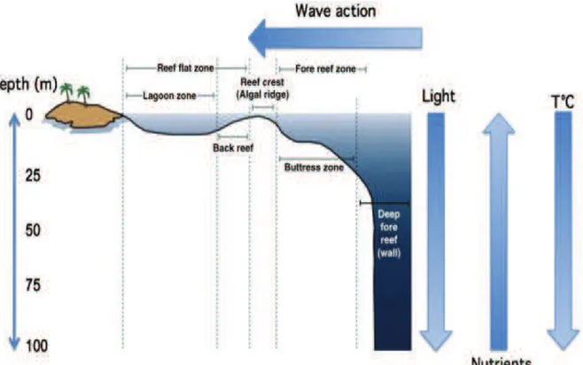
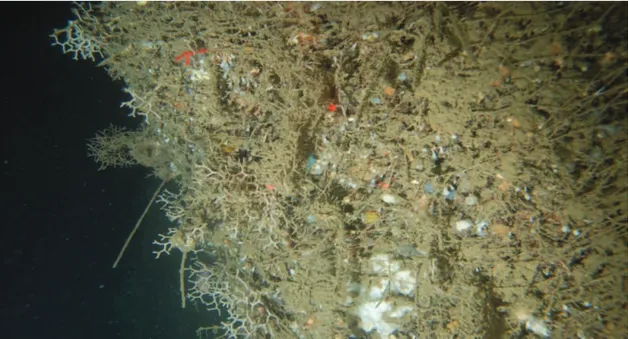
Mesophotic coral ecosystems (MCEs; Figure 1.1) are characterized by the presence of light dependent corals and associated communities typically found at water depths where light penetration is low (from 30-40 m and extending to around 150 m in tropical and subtropical regions) (Lesser et al. 2009; Hinderstein et al. 2010).The term mesophotic literally means “meso”, for middle, and “photic” for light. The dominant communities providing structural habitat in the mesophotic zone can be made up of corals, sponges, and algal species (Hinderstein et al. 2010). These habitats may be colonized by a number of species that are only found within this depth range and geographical location; moreover, both shallow-water and depth restricted species can be found (Brokovic et al. 2007). Intrinsically valuable as biodiversity hot-spots, they are important from a conservation perspective and provide home for a vast range of marine species (Hinderstein et al. 2010; Khang et al 2010; Rooney et al. 2010) (Fig. 1.2). Moreover, mesophotic coral ecosystem could provide a source of propaguls (larvae and recruits) to the shallow water habitats, favoring their recovery and resilience against human impact (Slattery et al. 2011). In fact, it has been hypothesized that MCEs may serve as potential source to replenish degraded shallow-water coral reef species, and are currently under study to evaluate their potential as refugia and/or larval supplier for shallow-water assemblages (Bongaerts et al. 2010; Miller et al. 2011; Van Oppen et al. 2011; Slattery et al. 2011).

4

Figure 1.1 Coral reef zonation showing gradients of light, nutrients and temperature with changes in depth from shallow reefs to mesophotic depths (From Lesser 2009).

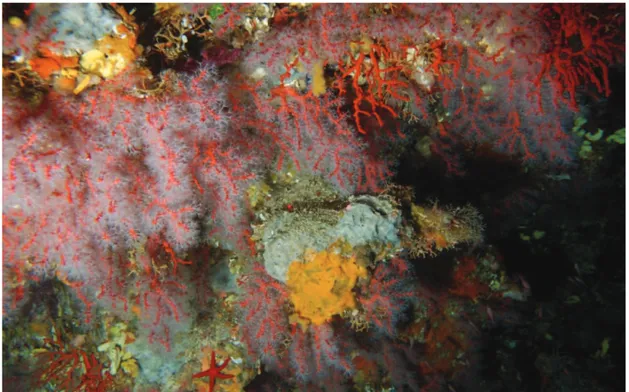
Figure 1.2 Coralligenous habitats dwelling in the mesophotic zone in the Mediterranean Sea (Picture made by Simone Canese, in Capel Rosso site at 60m depth).

Connectivity between shallow-water and deep-water populations is a fundamental prerequisite to consider MCEs as refugia because deep populations can act

5

as source of propagules for threatened shallow-water populations (Hinderstein et al. 2010). Furthermore, studies addressing these hypotheses provided conflicting results, depending on the analyzed coral species and on the geographic areas considered. Some studies show isolation between shallow and deep-water populations (Costantini et al. 2010; Costantini et al. 2011; Miller et al. 2011), whereas other studies shown the occurrence of gene flow (larval flow) between mesophotic and shallow-water ecosystem (Armstrong et al. 2006).

1.3 Mediterranean mesophotic habitats

The occurrence of mesophotic habitat in the Mediterranean Sea was reported since the first deep sea exploration (Marsili 1725). However, the exploration of these habitats and quantitative and experimental studies on their structure (Balata et al. 2005; Lineares et al. 2005) and dynamics (Airoldi 1998; Virgilio et al. 2006) were developed only when SCUBA diving techniques became available for scientific diving.

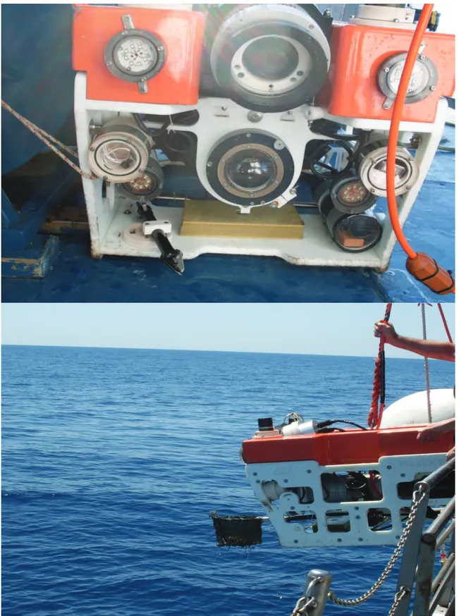
Remotely operated vehicles (ROVs) (Fig.1.3) allow extensive surveys in a depth range that is inaccessible to scuba diving, increasing the working depth range to more than 100m (Pyle 2000). The use of ROVs on small research vessels, allowed the exploration of MCEs in the coastal zone of the Mediterranean Sea; increasing in the last years the number of studies that have focused on MCE. Some of these studies describe the megabenthic biodiversity of the mesophotic zone in some areas of Mediterranean Sea (Bo et al. 2009; Bo et al. 2011 a, b, c), other investigate their structure, dynamics and genetic characterization (Freiwald et al. 2009; Gori et al. 2011; Cerrano et al. 2010; Costantini et al. 2010; Costantini et al. 2011).

6

Figure 1.3 The ROVs used in oceanographic cruises (May and June 2012) by the R/V Astrea. (Picture made by Simone Canese).

7

2. Corallium rubrum

2.1 Ecology

The red coral Corallium rubrum (Linneus 1758), belongs to the phylum Cnidaria (Anthozoa, Octocorallia, Scleraxonia), is a long-lived, slow growing gorgonian species. It represents one of the key ecosystem engineering species of coralligenous assemblage (a calcareous formation of biogenic origin), which is one of the richest Mediterranean habitat (Ballesteros 2006; Airoldi & Beck 2007). The origin of the actual distribution of red coral populations may date back to about 5 million years ago, when a coralligenous ecosystem replaced the coral reefs (Mateu 1986). Coralligenous is formed mainly due to the accumulation of encrusting calcareous algae in poorly lit areas and in relatively calm waters (Balata et al. 2005). The complexity of the structure of coralligenous allows the development of extremely heterogeneous communities, exhibiting high species richness and functional diversity (Gili & Coma 1998), dominated by "suspension feeders" (sponges, hydroids, anthozoans, serpulids, molluscs and tunicates) (Fig.2.1).

Corallium rubrum is a suspension feeder with passive filtration (Tsounis et al. 2005). The suspension feeders community evolved towards a complex three-dimensional structure, creating a barrier between the substrate and the water column so it interacts with the water column in littoral ecosystems by depleting food particles and transferring energy from the water column to the benthos (e.g. Cloern 1982; Oƥcer et al. 1982; Fre'chette et al. 1985,1989; Kimmerer et al. 1994; Riisga˚rd et al. 1998). In addition, these organisms create the habitat for vagile fauna of the coralligenous and increase the biomass and biodiversity of communities, structuring and stabilizing the ecosystem with their three-dimensional structure (Gili & Coma 1998; Arntz 1999).

8

Fig.2.1Coralligenous assemblages with some colonies of red coral. (Picture made by Simone Canese, in Capel Rosso site at 60m depth).

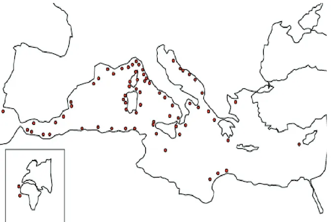
Corallium rubrum is a endemic Mediterranean species, mainly localized in Western Mediterranean Sea, in some parts of the Eastern Mediterranean Sea (Greek coast of the North Aegean Sea) and in the Atlantic coasts of south Portugal, Canary Islands, Mauritania, Senegal and Cape Verde Islands (Fig.2.2).

9

Figure 2.2: Geographical distribution of Corallium rubrum. The red circles represent the known populations (Marchetti 1965).

The distribution of the species shows major gaps related to the presence of stretches of sandy shores (e.g. Gulf of Valencia, Gulf of Lion, Versilia plain, Gulf of Gaeta) (Chintiroglou et al 1989; Marchetti 1965; Zibrowius et al. 1984). Moreover, red coral has strong habitat requirements , defined by the morphology and biogenic nature of the substratum, as well as by a series of abiotic variables (e.g. light intensity, water temperature and turbidity, sediment loads, current regime) (Weinberg 1979; Laborel & Vacelet 1961; Stiller & Rivoire 1984). It has a wide bathymetric distribution: from a few meters to about 800 m (Costantini et al. 2010). In shallower waters it is frequent in caves and poorly lit overhangs. Deeper down, it is found on underwater cliffs and even on the bottom (Laborel et Vacelet 1961; Zibrowius et al. 1984).

10

At the moment, three typologies of red coral populations have been described:

1. Shallow-water populations, in a depth range between 15 and 60 m, dwelling in vertical cliffs and inside caves; these populations have been commercially exploited for centuries and, at present, are made by small, short-lived colonies (Santangelo & Abbiati 2001);

2. Intermediate-water or mesophotic populations, at a depth range of 60 - 300 m, may be larger, sparse, long-lived colonies (Santangelo et al. 1999; Tsounis et al. 2006a);

3. Deep-water populations, below 300 m depth. These populations, for obvious practical reasons, are poorly known (Costantini et al. 2010).

Due to its commercial and ecological value, the biological information on the species increased noticeably during the last decades. Several studies have been carried out in different areas of the Mediterranean, mainly on its feeding ecology (Tsounis et al. 2006b), reproductive patterns (Vighi 1972; Santangelo et al. 2003; Torrents et al. 2005), recruitment (Garrabou & Hermelin 2002; Bramanti et al. 2005, 2009), growth (Bramanti et al. 2005), physiology (Rossi & Tsounis 2008), genetic population structure (Abbiati et al. 1993), competition for space (Giannini et al. 2003) and population dynamics (Santangelo et al. 2003). All these studies were carried out on shallow-water populations, and, until now, only few studies have focused on deeper populations (Garrabou et al. 2001; Bramanti et al. 2005; Tsounis et al. 2006b; Rossi et al. 2008; Torrents et al. 2008; Costantini et al. 2010, 2011).

11

2.2 Biology and reproduction

Red coral lives in compact colonies, each coral colony being formed by up it thousands of individual, white transparent polyps, each one bearing eight tentacles that produce a red skeleton of calcareous spicules. All polyps of a same colony are genetically identical (fig. 2.3).

Figure 2.3 Colonies of Corallium rubrum with expanded polyps (Picture made by Simone Canese, in Capel Rosso site at 60m depth).

Unlike other Cnidarians, red coral exhibits very limited organ development. It shares two anatomical features with other Cnidarians: a gastrovascular cavity (simple stomach) that opens only on one end, and a ring of tentacles. Red coral has no central nervous system. Unlike many coral species, it doesn’t have the symbiotic algae zooxanthellae living within the coral tissue. Lacking zooxanthellae means that the coral must obtain food by another method. It feeds on particles of organic matter, suspended in the water, which are captured by their tentacles (fig. 2.4). They also occasionally capture and consume larger zooplankton.

12

Figure 2.4 White polips (Picture made by Simone Canese).

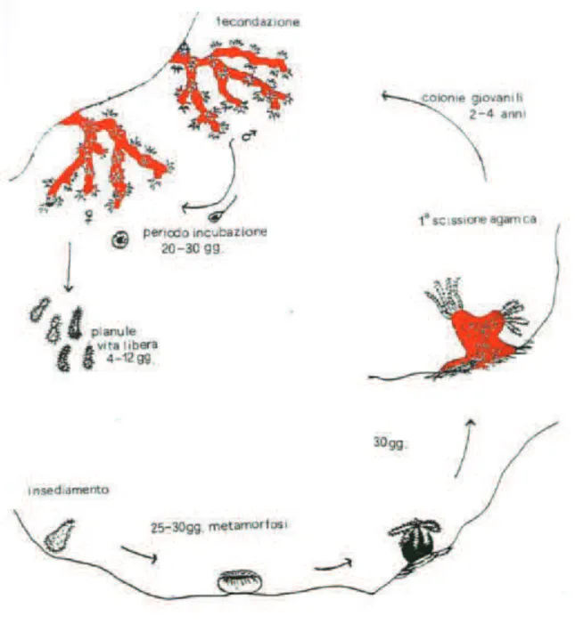
The reproductive system of the coral is inside the polyps. Although fragmentation is common in modular marine invertebrates (Jackson 1986; Karlson 1986), in red coral this has not been evidenced (Santangelo & Abbiati 2001). Recruitment in this species is therefore considered to depend on larval settlement (Santangelo et al. 2003). Sexes are normally separated in male and female colonies and, fertilization is internal, therefore fecundation happens when free-swimming sperm from male colonies reach the polyps of female colonies. The maturation of the male gametes takes place over one year. It starts at the beginning of summer. The maturation of the female gonads takes place every 2 years. It begins slowly the first year and is completed at the beginning of the second year (Vighi 1972). The fertilized eggs develop into larvae within the female polyp’s body cavity. The young larva, known as a planula, develops for 20 or 30 days inside the polyp before going out into the open sea. The emission of larvae takes place from July to the beginning of October, depending on the depth. The larvae swim for 4 to 15 days (Vighi 1972), or until they find a suitable substrate to settle. Like all larvae of sessile marine invertebrates, even the red coral planula requires specific conditions for settlement. Red coral planulae are indifferent to light and show negative geotropism and laboratory experiments suggest that larvae do not spread very far from the parental colonies (Vighi 1972), although, currently, limited data support or refute this hypothesis. Right after the settlement starts the metamorphosis, the mechanisms and control of which are totally unknown (Weinberg 1980). Following metamorphosis, the young larva begins to build-up its structure becoming a new coral colony.

13

The colony grows by asexual reproduction (fig. 2.5). The sexual maturity of the first polyps is reached after about 2 years (Santangelo et al. 2003).

14

2.3 Harvesting pressure and natural mortality

Since prehistoric times, man has been fascinated by red coral which, in spite of its mineral skeleton and vegetal aspect is, in reality, an animal. It was first used in the Upper Palaeolithic (approximately 20.000 B.C.). Later, it was represented on wall paintings and vases, or used to make jewellery and other objects by the Egyptians, the Greeks and the Romans (Morel et al. 2000). In the middle Ages, it was usual to carry a few pieces of coral in a bag to ward off witches. It was also used medicinally for its various supposed virtues. As a powder, for example, it was added to baby food as a protection from epidemics (Liverino 1983; Ascione 1993). Its use as a jewel and talisman has remained constant through the centuries (Roth 2002).

Nowadays, this species is still a resource of richness for many Mediterranean communities. Until quite recently, its professional fishers used a trawling gear called the Saint-André Cross. The Saint-André Cross consists of a wooden or, more recently steel, cross with nets attached. Trawled along the bottom at 50 m by boats, the Cross breaks the coral colonies and the pieces are caught by the nets. Such proceedings bring up 1 to 2 tons of coral a year. But the damage done on the bottom is too strong that in 1994 this kind of harvest method was banned. This important harvesting pressure resulted in profound changes in the species structure, switching from large colonies (base diameters of over 1 cm) into colonies with diameters of a few millimeters (Fig. 2.6.a, b).

Figure 2.6.a Low density of red coral individuals due to overexploitation in Campanian archipelago (picture made by Simone Canese).

15

Figure 2.6.b Dead red coral colonies in Campania archipelago (picture made by Simone Canese).

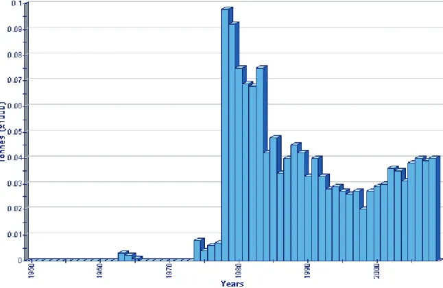
In 2008 was estimated that the annual quantity of red coral fished in the Mediterranean Sea is 400 tons (FAO, 2008, Fig.2.7).

16

The shallow water populations of the species are not subject to commercial fishing, but its high economic value, or simply its attractiveness to amateur divers has provoked over-exploitation also of these shallower populations, resulting in its complete disappearance from many places along our coasts.

The lack of adequate conservation and management measures could lead to the economical extinction of red coral but not to an ecological extinction (slow growth and density dependent species populations could survive to the overexploitation, but they could not reach the commercially exploitable size) (Santangelo et al. 2007). Meaningful conservation plans can only be built from knowledge of species life history traits (Torrents et al. 2004). Today, the shallow water populations are overexploited all over the Mediterranean Sea (Abbiati et al. 1992; Santangelo & Abbiati 2001; Tsounis et al. 2007; Tsounis et al. 2010; GFCM 2010) and the GFCM on 2010 has imposed a ban on red coral harvesting in populations shallower than 50 metres depth; moving the exploitation towards the mesophotic zone, where the harvesting is done by scuba divers which can immerse over 100m depth, and are capable of collecting up to 200-300kg a year in about 200 dives (http://www.centrescientifique.mc).

More than human overexploitation, there are other causes of natural origin that can lead to mortality of red coral colonies, including: crumbling of the substrate due to dwelling species, parasitism or endosymbiosis by boring sponges, increased sedimentation and mass-mortality events (Harmelin 1984). There are two species closely associated with red coral (Abbiati & Santangelo 1992): Pseudosimnia carnea (Poiret 1789), a gastropod that feeds on gorgonacea (Santangelo & Navarra 1984), and Balssia gasti (Balss 1921), a decapod crustacean that probably feeds on coenosarc (Santangelo et al. 1993). Moreover, many species of boring sponges (Demospongiae, Clionidae) penetrate in the coral sclerasse, seriously damaging it and reducing its commercial value. These organisms especially affect shallow-water populations, where the overunning by sponges starts from the calcareous substratum and then extends to coral (Corriero et al. 1997).

Furthermore, red coral populations were severely affected by mass mortality events occurring at the end of the summers of 1999 and 2003 along the French and Ligurian coasts. These events might have been related with the increase of temperature recorded in those areas (Cerrano et al. 2000; Perez et al. 2000; Garrabou et al. 2001), greatly impacting the population dynamics of this species (Santangelo et al. 2007).

17

Red coral shows a good resilience in cases of reduction of the reproductive output and increased mortality, a typical feature in species with low growth rates, high rates of reproduction and overlapping generations. Sporadic mortality events affect its survival, but the increase of fishing pressure and frequent mass mortality events may cause serious damage over time because the recovery potential of the species may not be sufficient to balance them (Santangelo et al. 2007; Tsounis et al. 2007).

2.4 Population genetic

Previous genetic studies on red coral populations investigated its effective larval dispersal as well as the spatial genetic structure between and within different geographical areas. Based on the use of allozymes, significant differentiation was observed between samples separated by about 10 km (Abbiati et al. 1993). Successively, using more variable molecular markers, a genetic structuring at scales of less than one meter was observed. Moreover, a high inbreeding rate within populations was also detected (Costantini et al. 2007; Ledoux et al 2010a, b). The inbreeding is the reproduction between closely related individuals or next-to-kin, and probably represents an evolutionary adaptation as it has the effect of bringing to homozygosity genetic loci: this homozygosity makes that both favorable and deleterious genes are enhanced and, if the last are prevalent, could have serious negative effects for the populations survival.

At Mediterranean scale a genetic structuring among shallow-water populations with some isolation by distance patterns (Ledoux et al. 2010a, b) was observed (Costantini et al. 2007b) confirming its patchy distribution. Together, these results suggested that red coral larvae have a short dispersal capability and that the populations tend to be self-recruiting. Recently, studies on deeper populations showed a decline of genetic variability along a depth gradient in a range between 20-70 meters and a genetic isolation between shallow and deep-water populations, suggesting that depth might have an important role in determining the patterns of genetic structure of the species (Costantini et al. 2010).

18

AIMS

Since shallow water red coral populations are overexploited along all the Mediterranean coasts, today the harvesting pressure has moved towards the deeper populations. Nevertheless, these mesophotic populations are still understudied, when compared to their shallow-water counterparts.

The aim of this thesis is to fill gaps in the knowledge on the biology and ecology of currently harvested red coral populations using a genetic approach. Research cruises were done to sample red coral colonies distributed in three different areas of the Western Mediterranean Sea and in a depth range from 60 to 120 metres. In particular, two molecular markers with different levels of polymorphism, the mitochondrial control region and 12 microsatellite loci were used to evaluate the genetic variability and structuring of the populations.

These data together with those obtained on population structure, biology and ecology will be very useful to allow appropriate management of the harvesting of this precious resource.

19

4. MATERIALS AND METHODS

3.1 Sample collection

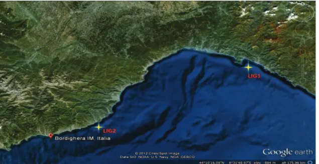
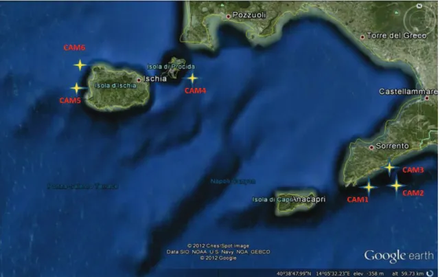
Three different geographic areas along the Tyrrhenian Sea were selected for oceanographic cruises done between May and June 2012 by the R/V Astrea: Ligurian coast, Tuscan Archipelago, and Campania coast (Figure 3.1. a, b, c). These surveys were specifically dedicated to the sampling of mesophotic red coral populations. Corallium rubrum colonies were sampled at 14 sites corresponding to different habitats (overhangs, vertical cliffs and outcrops; Table 3.1). The areas are separated among them by hundreds of kilometers and the sampling sites within each area were separated by tens to hundreds of meters. The occurrence of Corallium rubrum was detected by a multibeam echosounder and in total 148 red coral colonies were sampled using a Remotely Operated under water Vehicle (ROV), at depth ranging between 60 and 120 metres (Table 3.1). For each site, a branch fragment from 6 to 23 live colonies of red coral was collected within an area ranging from 50 to 100 m2. The difference in the number of colonies sampled for each site depends to the abundance of the species. All the fragments were preserved, after collection, in 80% ethanol at 4°C for subsequent molecular analyses.

20

Figure 3.1.a Map showing the Liguria sample area. Yellow stars indicate the position of sampled populations.

Figure 3.1.b Map showing the Toscana sample area. Yellow stars indicate the position of sampled populations.

21

Figure 3.1.c Map showing the Campania sample area. Yellow stars indicate the position of sampled populations.

CODE SITE AREA LATITUDE LONGITUDE DEPTH (m) SAMPLES

LIG1 Portofino P.Faro (GE) Liguria 44°17.80'N 9°12.140'E 68 6 LIG2 Bordighera (IM) Liguria 43°44.67'N 7°40.917'E 73 9 TOS1 Isola del Giglio (GR) Toscana 42°18.64'N 10°55.19'E 105 13 TOS2 Pianosa Nord (LI) Toscana 42°38.40'N 10°6.49'E 73 6 TOS3 Scogliosante Toscana 42°25.08'N 10°04.81E 85 11 TOS4 Montecristo (LI) Toscana 42°30.84'N 10°18.63'E 120 10 TOS5 TunaParadive (LI) Toscana 42°17'N 10°14'E 94 23 TOS6 Capel Rosso (LI) Toscana 42°18.07'N 10°19.10'E 60 6 CAM1 Li galli (SA) Campania 40°34.71'N 14°25.18'E 100 7 CAM2 Li galli (SA) Campania 40°34.52'N 14°25.03'E 100 6 CAM3 Li galli (SA) Campania 40°34.62'N 14°24.69'E 90 9 CAM4 Punta Solchiaro (NA) Campania 40°44.27'N 14°01.09'E 60 15 CAM5 Punta Imperatore (NA) Campania 40°42.246'N 13°50.94'E 108 6 CAM6 Scoglio D'Ischia (NA) Campania 40°43.72'N 13°49.52'E 73 6

Table 3.1 Codes, sites, areas, coordinates, depth and number of individuals collected during the oceanographic campaigns.

22

3.2 Dna extraction and molecular analysis

Total genomic DNA was extracted from two to four polyps per individual colonies using cetyltrimethyl ammonium bromide (CTAB) protocol (Winnepenninckx et al. 1993) following the procedure described in Costantini et al. (2007b). Total DNA was visualized in a 0.8% agarose gel, stained with GelRed (BIOTIUM) 1%, after a 30 minutes electrophoresis at 120 V. Extractions were loaded with the loading buffer BLU 6X. Gene Ruler Express DNA Ladder was used for sizing and quantification of DNA

fragments. The extraction product was diluted to 1:20 and 1:50 in ultrapure water

(SIGMA) for better amplification success.

Eleven microsatellite loci (COR9, COR46, COR58, COR15, MIC23, MIC22, COR48, MIC26, MIC24, MIC13, MIC20) specifically developed for Corallium rubrum (Costantini & Abbiati 2006; Ledoux et al. 2010a) and one (CR3Al7) developed for Corallium lauuense (Baco et al. 2006) were analyzed. Microsatellite loci were amplified in multiplex with a QIAGEN® Multiplex PCR Kit using polymerase chain reaction (PCR) (conditions described in Costantini et al. 2011). Genotyping of individuals was carried out on an ABI 310 Genetic Analyser (Applied Biosystems), using forward primers labeled with FAM, HEX/VIC, TAMRA/NED, ROX/PET (Sigma) and LIZ HD500 (Applied Biosystems) as internal size standard. Allele sizing was conducted using Peak Scanner Analysis Software v1.0 (Applied Biosystems).

The mitochondrial control region (MtC) sequences were amplified using the primers ND618510CkonojF 5’-CCATAAAACTAGCTCCAACTATTCC-3’ and COI16CkonojR 5’-GGTTAGTAGAAAATAGCCAACGTG-3’ (Sigma). These primers were specifically designed using the online PRIMER3 version 4.0 software (Rozen & Skaletsky 2000) on the nad6 and cox1 genes flanking the putative control region, which seems located in the intergenic spacer 12 (IGS12) of the mitochondrial genome of Paracorallium japonicum and Corallium konojoi (Uda et al. 2011). Each 25.0 μL MtC PCR reaction contain: 2.5 µL of DNA template; 2.5 µL of buffer; 2 µL of MgCl2 25 mM; 2 µL of dNTPs 10 mM; 1.25 µL of each forward and reverse primers 10 mM; 13.3 µL of ultrapure water (SIGMA) and one unit (0.2 µL) of Taq polymerase enzyme (Invitrogen). PCR reaction was performed in a GeneAmp® PCR Sistem 2700 thermocycler (Applied Biosytems) as follows: an initial denaturation at 95 °C for 3 min, 30 cycles including 95 °C for 30 s, other 30s at a specific annealing temperature 59 °C and an extension at 72 °C for 60 s, and a final extension at 72 °C for 7 min. After PCR,

23

the products were maintained at 4ºC. Products of amplification were visualized in a 1.5% agarose gel as previously described. PCR products were sent to Macrogen (South Korea) for purification and sequencing with the same primers using for the amplification.

3.3 Microsatellite Markers

3.3.1 Genetic Variability

Sampling using the ROVs may cause fragmentation of the colonies, and in some cases we can wrongly analyze fragments belonging to the same individual as if they were from different colonies. For this reason first of all individuals sharing the same multilocus genotype (MLG) were checked using GENALEX version 6.1 (Peakall & Smouse 2006). Moreover, the unbiased probability of identity (PID Kendall & Stewart 1977) that two individuals share the same MLG by chance and not by descent was computed.

The analysis of microsatellite genetic variability within samples were estimated evaluating the number of alleles for locus and populations (Na), observed heterozygosity (Ho) and unbiased gene diversity (Hs, Nei 1987) using the GENETIX software package version 4.05 ( Belkhir et al. 2004). Single and multilocus Fis were estimated using Weir and Cockerham’s model (Weir & Cockerham 1984) implemented in GENETIX. Fis give us information about populations equilibrium, with values ranging from -1 to 1 (where values near to 0 means that Ho is close to Hs). Since several Fis values obtained are positive (Ho < Hs), the departures from Hardy-Weinberg equilibrium (HWE) were tested using “Fisher’s exact test” in GENEPOP version 3.4 (Raymond & Rousset 1995) as implemented for online use (http://genepop.curtin.edu.au/), with the level of significance determinate by a Markov-chain randomization. For this analysis 1000 steps of dememorization, 100 batches and 1000 iterations per batch, were set, with the aim to obtain a significance level of 1%. Moreover, significant differences in genetic diversity (Ho, Hs, Fis) among populations grouped according to their geographical origin (two populations for Liguria; six populations for Toscana and Campania respectively) were tested using a permutation procedure (1000 iterations) in FSTAT version 2.9.3.2 (Goudet 2001).

24

3.3.2 Population genetic differentiation

The genetic divergence among populations was determined from the original dataset using Weir & Cockeram’s (1984) FST estimator in the ARLEQUIN Version 2.0 software (Schneider et al. 1999). FST values ranges from0 to 1. A zero value implies complete panmixia; while a value of 1 would implies that the two populations are completely separate. The significance of the estimator was determined using bootstrap resampling with 10000 permutations.

To evaluate the isolation by distance pattern, and so the presence of correlation among genetic differentiation estimates (FST) and geographical distance (Log transformed), a Mantel test (Mantel 1967) computed using the Isolde program implemented in GENEPOP (using 1000 permutations to test the significance level of correlation) was used.

The programme STRUCTURE v. 2.3 was used to detect the number (K) of genetically homogeneous populations in the microsatellite dataset (Pritcherd et al. 2000, Falush et al. 2003, 2007). Each individual was assigned to probable common clusters based on the similarity of their multilocus genotypes at 10 microsatellite loci. Mean and variance of log likelihoods of the number of clusters for K=1 to K=16 were inferred from multilocus genotypes by running STRUCTURE five times with 200000 repetitions each (burn-in=50000 iterations) under the admixture ancestry model and the assumption of correlated allele frequencies among samples (as suggest in Falush et al. 2003).

In order to have a visual assessment of between-population differentiation, we performed a discriminant analysis of principal components (DAPC, Jombart et al. 2010) as implemented in the ADEGENET package for R (Jombart 2008). This technique extracts information from genetic datasets (multivariate in nature) by first performing a principal component analysis (PCA) on pre-defined groups or populations, and then using the PCA factors as variables for a discriminant analysis (DA), which seeks to maximize the intergroup component of variation. The optimal number of clusters (populations) was predicted using the k-means clustering algorithm, find.clusters’, retaining all principal components. In all analyses 50 principal components of PCA were retained as input to DA.

25

The partition of genetic variance among samples was conducted through an analysis of molecular variance (AMOVA) implemented in ARLEQUIN. For this purpose three different AMOVA were computed: the first, grouping populations based on their geographical origin (three different areas: Liguria-LIG, Toscana-TOS and Campania-CAM); the second, grouping populations according to the STRUCTURE results (two groups: LIG-TOS populations and CAM populations) and the third grouping populations according to the DAPC results (three group: LIG1-2 and TOS1-2 populations; TOS3-4-5-6; and CAM populations). The AMOVA assigns percentages of variability explained and a significance to the variability among groups, within populations inside the groups and within populations without grouping, giving information on the degree of homogeneity of the groups set and how differentiated are from each other.

3.4 Mitochondrial Markers

3.4.1 Genetic variability

The obtained sequences were edited and aligned manually using BioEdit Sequence Alignment Editor v. 7 (Hall 1999). The alignment was performed with ClustalX (Thompson et al. 1997) and corrected by hand.

Sequence genetic diversity within samples was estimated using number and of haplotype (h), haplotype diversity (Hd, Nei 1987) and nucleotide diversity (π, Nei 1987) using DnaSP v5.10 software (Librado & Rozas 2009). The value of Hd ranges from 0 to 1. A value of 0 indicates that all haplotypes are identical (no diversity), while a value of 1 (very high diversity) indicates no shared haplotypes among individuals (Grant & Bowen 1998). The nucleotide diversity (Pi or π) is the average sequence divergence among haplotypes (Grant & Bowen 1998).

26

3.4.2 Population genetic differentiation

Population differentiation was analyzed using pairwise genetic distances (FST) between populations, in ARLEQUIN 3.5 (Excoffier et al. 2005). The significance of the genetic distances was tested by permuting 10000 times the haplotypes between the populations, assuming as null hypothesis (H0) the absence of population differentiation. The P-value of the test was the proportion of permutations leading to FST values larger or equal to the observed ones. If P-values <0.05 (significant) or 0.01 (highly significant), the H0 is rejected hence the pair of populations compared are significantly different.

In order to have a visual assessment of between-population differentiation a Multidimensional Scaling (MDS) were performed using the software PRIMER v6 (Clarke 1993).

With the intent to detect the effect of isolation by geographical distance, we compared the correlation of genetic distances (Reynold’s distance: FST /1- FST) with log10-transformed geographical distances using the Mantel test procedure implemented in GENEPOP version 4.1 (Rousset 2008).

The partition of the genetic variance among areas was conducted through an analysis of molecular variance (AMOVA) implemented in the ARLEQUIN software v3.5.1.2 (Excoffier & Lischer 2010) grouping population for their geographical origin (three groups) and grouping populations according MDS results.

27

4. RESULTS

4.1 Microsatellite Markers

4.1.1 Genetic Variability

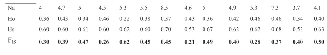
A total of 148 Corallium rubrum colonies were analyzed. The twelve microsatellite loci analyzed were polymorphic in all fragments. Loci MIC22 and MIC23 were excluded from subsequent analysis, because they correctly amplified in Toscana and Liguria populations, but did not give any amplification in Campania populations. Over all samples, the number of alleles per locus ranged from 1 (COR15, COR58 and MIC13) to 17 (MIC26). Within populations, over all loci, the mean number of alleles ranged between 3.7 (in CAM5) and 8.5 (in TOS5). Mean observed heterozygosity ranged between 0.22 (in TOS3) to 0.46 (in TOS2, CAM3, CAM4), and gene diversity from 0.53 (in TOS6, CAM5) to 0.70 (in TOS5) (Tab. 4.1).

SAMPLE (n) CAM6 (6) LOCUS LIG1 (6) LIG2 (9) TOS1 (13) TOS2 (6) TOS3 (11) TOS4 (10) TOS5 (23) TOS6 (6) CAM1 (7) CAM2 (6) CAM3 (9) CAM4 (15) CAM5 (6) COR9 bis N 6 7 10 6 5 8 16 5 7 6 8 14 6 5 Na 5 3 4 5 5 5 9 3 7 5 4 7 6 5 Ho 0.16 0.14 0.20 0.33 0.40 0.12 0.31 0 0.28 0.50 0.75 0.64 0.66 0.40 Hs 0.79 0.35 0.68 0.72 0.68 0.57 0.81 0.56 0.75 0.72 0.67 0.67 0.73 0.60 FIS 0.82 0.64 0.73 0.60 0.50 0.80 0.63 1 0.66 0.38 -0,05 0.07 0.18 0.42 COR15 N 5 7 13 6 10 10 19 4 5 5 4 15 6 4 Na 2 3 2 2 1 1 2 4 2 4 3 3 2 3 Ho 0 0.42 0.15 0.33 0 0 0 0.25 0.20 0.20 0.25 0.06 0 0.25 Hs 0.48 0.50 0.26 0.27 0 0 0 0.21 0.66 0.18 0.65 0.18 0.27 0.59 FIS 1.00 0.21 0.44 -0.11 - - - - 0.75 - 0.70 0.65 1.00 0.66 COR46bis N 3 7 8 2 11 10 20 6 7 6 9 11 6 3

28 Na 3 8 6 2 4 9 12 8 10 6 9 15 5 6 Ho 0.66 0.71 0.25 0.50 0 0.60 0.45 0.50 0.71 0.50 0.66 0.81 0.33 1 Hs 0.61 0.84 0.71 0.37 0.62 0.81 0.87 0.84 0.88 0.77 0.86 0.92 0.77 0.83 FIS 0.11 0.23 0.68 - 1.00 0.31 0.50 0.48 0.26 0.43 0.28 0.15 0.62 0 COR48 N 6 9 9 6 10 7 10 4 7 6 5 8 5 5 Na 7 9 9 8 8 6 10 7 4 6 7 8 8 6 Ho 0.33 0.55 0.33 0.66 0.40 0.71 0.60 0.75 0.14 0.50 0.60 0.37 0.80 0.40 Hs 0.83 0.86 0.75 0.86 0.78 0.74 0.84 0.84 0.72 0.75 0.84 0.82 0.86 0.80 FIS 0.52 0.40 0.60 0.31 0.52 0.11 0.33 0.25 0.82 0.41 0.38 0.58 0.17 0.57 COR58 N 4 6 10 4 4 7 8 3 4 3 6 13 0 4 Na 3 4 4 5 4 6 8 1 4 3 3 5 0 3 HO 0 0.33 0.30 0.50 0 0.28 0.25 0 0 0 0.16 0.07 0 0.25 Hs 0.62 0.41 0.74 0.78 0.75 0.69 0.82 0 0.75 0.66 0.40 0.61 0 0.59 FIS 1.00 0.28 0.62 0.47 1.00 0.63 0.73 - 1.00 1.00 0.64 0.88 - 0.66 MIC13 N 5 7 10 3 7 6 22 6 2 3 4 7 5 3 Na 1 2 4 1 2 2 4 3 2 2 3 4 3 3 Ho 0 0 0.20 0 0 0 0.27 0.33 0.50 0 0.50 0.28 0 0.33 Hs 0 0.24 0.66 0 0.40 0.27 0.57 0.29 0.37 0.44 0.40 0.66 0.64 0.50 FIS - 1.00 0.72 - 1.00 1.00 0.54 -0,05 - 1.00 -0,09 0.61 1.00 0.50 MIC20 N 6 7 11 6 10 10 20 6 7 6 9 13 3 4 Na 4 5 3 8 9 7 8 4 4 8 8 7 4 4 Ho 0.83 0.42 0.09 0.66 0.50 0.40 0.50 0.66 0.28 0.83 0.22 0.69 0.66 0.75 Hs 0.58 0.76 0.16 0.86 0.83 0.80 0.76 0.68 0.64 0.84 0.82 0.81 0.66 0.65 FIS -0.35 0.50 0.50 0.31 0.44 0.53 0.37 0.11 0.60 0.10 0.75 0.18 0.20 0 MIC24 N 6 8 6 6 10 6 23 6 7 6 9 14 6 5 Na 3 4 3 5 7 8 7 3 5 4 2 6 2 4 Ho 1 0.75 0.66 0.50 0.50 1 0.43 0.66 0.42 0.33 0.11 0.28 0.16 0.40 Hs 0.56 0.67 0.56 0.61 0.65 0.84 0.71 0.48 0.61 0.51 0.10 0.61 0.15 0.58 FIS -0.71 -0.05 -0.08 0.26 0.28 -0.09 0.41 -0.29 0.37 0.43 - 0.56 - 0.40 MIC26 N 6 6 12 6 10 7 17 6 7 6 9 12 5 6 Na 6 4 6 6 10 9 17 10 8 8 8 11 3 3 Ho 0.33 0.33 0.58 0.66 0.40 0.71 0.76 0.83 0.71 0.66 0.33 0.58 0.40 0 Hs 0.77 0.68 0.78 0.81 0.90 0.85 0.90 0.87 0.79 0.83 0.78 0.85 0.54 0.50 FIS 0.62 0.57 0.29 0.27 0.59 0.24 0.18 0.13 0.17 0.28 0.61 0.35 0.36 1.00 CR3AL7 N 6 6 11 2 9 7 20 3 7 6 9 15 5 5 Na 6 5 9 3 3 2 8 3 4 3 6 7 4 4 Ho 0.33 0.66 0.63 0.50 0 0 0.15 0.33 0.42 0.66 1 0.86 0.40 0.20 Hs 0.75 0.66 0.79 0.62 0.56 0.40 0.65 0.50 0.53 0.48 0.67 0.65 0.66 0.70 Fis 0.61 0.09 0.24 0.50 1.00 1.00 0.78 0.50 0.26 -0.29 -0.42 -0.3 0.48 0.76

29 Multilocus Na 4 4.7 5 4.5 5.3 5.5 8.5 4.6 5 4.9 5.3 7.3 3.7 4.1 Ho 0.36 0.43 0.34 0.46 0.22 0.38 0.37 0.43 0.36 0.42 0.46 0.46 0.34 0.40 Hs 0.60 0.60 0.61 0.60 0.62 0.60 0.70 0.53 0.67 0.62 0.62 0.68 0.53 0.63 FIS 0.30 0.39 0.47 0.26 0.62 0.45 0.45 0.21 0.49 0.40 0.28 0.37 0.40 0.50

Highly significant deviations from HWE (P < 0.001) were observed in all populations with Hs significantly higher than Ho. All multilocus estimates of FIS were significant different from 0 and ranged from 0.21 (in TOS6) to 0.62 (in TOS3), showing heterozygote deficiencies in all analyzed samples (Table 4.1).

No significant difference in genetic diversity (Ho, Hs, FIS) were observed among populations belonging the different areas (P > 0.05, data not shown).

4.1.2 Population genetic differentiation

Analysis of genetic differentiation between pairs of populations showed value of FST between 0 (TOS2 with TOS6 and CAM5, CAM4 with CAM2 and CAM5) to 0.24 (among CAM6 and TOS1) (Table 4.2) with major pairwise comparison significantly different (P<0.01).

Mantel test showed a statistically significant correlation between geographic distance and genetic differentiation among populations (p=0; Fig.4.1).

Table 4.1 Summary of genetic diversity at ten microsatellite loci within Corallium rubrum populations: n, number of sampled individuals; N, number of genotypes per locus; Na, number of alleles per locus; Ho, observed heterozygosity; Hs, gene diversity (Nei 1987); FIS, Weir and Cockerham's (1984) estimate

30

LIG1 LIG2 TOS1 TOS2 TOS3 TOS4 TOS5 TOS6 CAM1 CAM2 CAM3 CAM4 CAM5 CAM6 LIG1 LIG2 0.08 TOS1 0.17 0.12 TOS2 0.08 0.01 0.05 TOS3 0.09 0.12 0.08 0.3 TOS4 0.17 0.21 0.12 0.10 0.05 TOS5 0.08 0.07 0.06 0.5 0.01 0.01 TOS6 0.05 0.08 0.13 0 0.05 0.15 0.07 CAM1 0.14 0.13 0.15 0.10 0.13 0.17 0.06 0.11 CAM2 0.12 0.12 0.13 0.03 0.09 0.16 0.05 0.07 0.07 CAM3 0.11 0.14 0.18 0.05 0.12 0.20 0.12 0.09 0.10 0.02 CAM4 0.15 0.14 0.14 0.06 0.06 0.11 0.05 0.05 0.06 0 0.08 CAM5 0.09 0.14 0.07 0 0.09 0.12 0.09 0.10 0.08 0.01 -0.02 0 CAM6 0.16 0.18 0.24 0.14 0.16 0.22 0.10 0.11 0.02 0.04 0.05 0.08 0.04 0

Table 4.2 Pairwise multilocus estimates of FST (Weir & Cockerham 1984) between all samples. Bold values are statistically significant (P < 0.01).

Figure 4.1 Relationship between genetic differentiation and the logarithm of geographical distance among Corallium rubrum populations for microsatellites markers.

R2 _{= 0.212} P = 0.00 -0,1 -0,05 0 0,05 0,1 0,15 0,2 0,25 0,3 0,35 -2 0 2 4 6 8 F s t/ (1 -F s t) Geografical distance (km)

Isolation by distance

31

Testing the significance of the stepwise clustering procedure performed in STRUCTURE resulted in a separation of the populations into two clusters (K=2, Δk=128.26) (Fig.4.2). First cluster contained Liguria and Toscana populations, while the second contained the remaining Campania populations (in according with geographical distance).

Figure 4.2 Results of the clustering analysis conducted in STRUCTURE. Each individual is represented by a vertical line partitioned into k-colored segments that represent the individual’s membership fraction in k clusters. Each population is delineated by black vertical lines and number representing populations in ascending order from Liguria to Campania.

The DAPC showed that the 50 principal components of the retained PCA explained 95 % of the total variance. The scatterplot of the first two components of the DA showed the same results of STRUCTURE. Nevertheless, from the graphic representation (Fig.4.3) can be seen as inside the first cluster there is a slight differentiation between one small cluster including all the samples from Liguria and two populations from Toscana (TOS1 and TOS2) and other small of only Toscana populations (TOS3, TOS4, TOS5, TOS6).

32

Figure 4.3 Plots of the first two axes obtained in the Discriminant Analysis of Principal Components using microsatellite dataset. Dots represent individuals.

The AMOVA test (Table 4.4) conducted among populations showed similar results independently or the grouping considered (see Materials for grouping). Major variability is explained within populations (between 89.06% and 89.93% depending of the grouping). Moreover, the variance among groups was always significant even if the percentage of variation is very low (between 4.43 and 6.09% depending of the grouping).

33

Source of variation d.f. Sum of squares Variance

component Percentage of variation Among groups 2 32.985 0.15 6.09*** Among sample 11 49.320 0.12 4.86*** within groups Within samples 252 563.496 2.24 89.06*** Total 265 645.8 2.51 *** P<=0.001

Table 4.3 Analysis of molecular variance (AMOVA) among Corallium rubrum populations using microsatellite data set. Red coral populations were grouped according to their geographical distribution (three groups: Liguria, Toscana and Campania populations).

34

4.2 Mitochondrial Markers

4.2.1 Sequence variation

Across 101 individuals amplified for the putative control region of the mitochondrial DNA (Table 4.5) the fragments was 290 bp in length. MtC in Corallium rubrum correspond to positions 18541-18913 of the mitochondrial genome sequence of Paracorallium japonicum (GenBank accession number AB595189, Uda et al. 2011) and to positions 18538-18702 and 18815-18969 of the mitochondrial genome sequence of Corallium konojoi (GenBank accession number AB595190, Uda et al. 2011). The sequence of the MtC in C. rubrum had a percentage of identity of 99% and 92% with those of P. japonicum and C. konojoi, respectively. The alignment of all individual sequences showed the presence of five nucleotide substitution which defines four different haplotypes (Table 4.5). The sequence alignment showed the presence of the three haplotypes (Hap1, Hap2, Hap3) previously recorded by Costantini et al. (2011). Haplotype 1 and 2 were present in almost all populations and were the most abundant (36% and 37% respectively). Haplotype 4 is only present in a population of Tuscany (TOS1), where it was the most abundant. Nucleotide diversity is slow, but this depends of the low number of variable position (only five). So, low and comparable value of haplotype and nucleotide diversity of MtC were found among populations, with mean values of 0.38 (± 0.14) and 0.0033 (± 0.0001) respectively.

3 5 N uc le o ti de p o si ti o n L IG 1 L IG 2 T O S 1 T O S 2 T O S 3 T O S 4 T O S 5 T O S 6 C A M 1 C A M 2 C A M 3 C A M 4 C A M 5 C A M 6 2 8 8 2 1 2 9 2 7 4 2 7 5 ( 6 ) (9) (13 ) (6) (11 ) (10 ) (23 ) (6) (7) (6) (9) (15 ) (6) (6) N .am p 6 6 13 6 2 5 15 4 7 5 9 13 6 4 H ap _ 1 C A C A G 4 4 0 5 2 4 1 4 0 2 0 0 1 0 0 H ap _ 2 T G . . . 2 2 0 0 0 1 1 1 2 4 7 8 5 4 H ap _ 3 T G . C T 0 0 5 1 0 0 0 3 3 1 2 4 1 0 H ap _ 4 T G T G T 0 0 8 0 0 0 0 0 0 0 0 0 0 0 h 2 2 2 2 1 2 2 2 3 2 2 3 2 1 H 0 .5 3 ± 0 .1 7 0 .5 3 ± 0 .1 7 0 .5 1 ± 0 .0 8 0 .3 3 ± 0 .2 1 0 0 .4 1 ± 0 .2 0 0 .1 3 ± 0 .1 1 0 .5 0 ± 0 .2 6 0 .7 6 ± 0 .1 1 0 .4 0 ± 0 .2 1 0 .3 ± 0 .1 0 .5 6 ± 0 .1 1 0 .3 3 ± 0 .2 1 0 π 0 .0 0 7 ± 0 .0 0 2 0 .0 0 7 ± 0 0 .0 0 5 ± 0 0 .0 0 2 ± 0 .0 0 1 0 0 .0 0 5 ± 0 .0 0 3 0 .0 0 2 ± 0 .0 0 1 0 .0 0 3 ± 0 .0 0 1 0 .0 0 6 ± 0 .0 0 1 0 .0 0 2 ± 0 .0 0 1 0 .0 0 2 ± 0 .0 0 2 0 .0 0 4 ± 0 .0 0 1 0 .0 0 2 ± 0 .0 0 1 0 T a b le 4. 4 S eque n ce di ff er en ce s, di st ri b ut io n a n d ge n et ic di v er si ty of t h e fo ur M tC ha p lo ty p es fo un d in C or al li um r ubr um p o p ul at io n s: do ts i ndi ca te i de n ti ca l b as es ; H , to ta l n u m b er o f ha p lo ty p es ; h , ha p lo ty p e di v er si ty ( h , N ei 19 87); π , nuc le o ti de di v er si ty ( π, N ei 1 9 87).

36

4.2.2 Genetic differentiation between populations

The MtC marker revealed low values of genetic differentiation, compared to microsatellites. Pairwise FST estimated ranged from -0.01 (CAM1 vs LIG1 and LIG2) to 1 (CAM6 vs TOS3) (Table 4.5).

.

LIG1 LIG2 TOS1 TOS2 TOS3 TOS4 TOS5 TOS6 CAM1 CAM2 CAM3 CAM4 CAM5 CAM6 LIG1 LIG2 -0.2 TOS1 0.45 0.45 TOS2 0.03 0.03 0.65 TOS3 -0.09 -0.09 0.66 -0.3 TOS4 -0.17 -0.17 0.55 -0.12 -0.29 TOS5 0.15 0.15 0.73 -0.07 -0.33 -0.04 TOS6 0.24 0.24 0.28 0.63 0.71 0.42 0.73 CAM1 -0.01 -0.01 0.31 0.29 0.29 0.12 0.47 -0.1 CAM2 0.4 0.4 0.36 0.78 0.83 0.59 0.82 0.31 0.23 CAM3 0.45 0.46 0.39 0.77 0.81 0.62 0.81 0.33 0.28 -0.18 CAM4 0.3 0.3 0.31 0.61 0.63 0.46 0.69 0.05 0.08 -0.08 -0.04 CAM5 0.45 0.45 0.39 0.8 0.85 0.63 0.83 0.39 0.29 -0.22 -0.15 -0.03 CAM6 0.53 0.53 0.47 0.89 1 0.72 0.89 0.67 0.42 -0.05 -0.01 0.11 -0.08 0

Table 4.5 Pairwise multilocus estimates of MtC between all Corallium rubrum populations. Bold values are significantly different from zero (P <=0.01).

The Multidimensional Scaling (MDS) representation (Fig.4.4), utilized with the intent to have a visual assessment of between-population differentiation, showed three groups of samples. First group includes Liguria (LIG1, LIG2) and several Toscana populations (TOS2, TOS3, TOS4, TOS5), second group with TOS1 and TOS6 (probably in according with the presence of Hap 4 only in TOS1, and the low number of haplotypes in TOS6) and third group with all Campania populations.

37

Figure 4.4 Multidimensional scaling of the pairwise FST among populations. Green triangle

represents Liguria populations, blue triangle Toscana populations and blue square Campania populations.

Even in this case, as in microsatellite dataset, the Mantel test was significant, so there is correlation between genetic and geographical distances (Fig.4.5).

38

Figure 4.5 Relationship between genetic differentiation estimates and the logarithm of geographical distance among Corallium rubrum populations using MtC dataset.

The AMOVA test (Table 4.7) conducted among populations even in this case showed major genetic variation within population (47.35%; P<0.001), while about 25% of variations is observed among groups (three geographical areas: Liguria, Toscana and Campania) and among populations within groups. The percentage of variation among group increase significantly grouping populations according the FST values and MDS results (53.45% , P = 0, data not shown).

R² = 0,0729 P=0,001 -1 0 1 2 3 4 5 6 7 8 9 -2 -1 0 1 2 3 4 5 6 7 F st /( 1 -F st ) Log distance (km)

Isolation by distance

39

Source of variation d.f. Sum of squares Variance

component Percentage of variation Among group 2 25.231 0.312 25.68* Among populations 11 31.215 0.328 26.96** within group Within populations 87 50.089 0.57 47.35** Total 100 106.5 1.21 *= P<0.05 **=P<0.001

Table 4.6 Analysis of molecular variance (AMOVA) among Corallium rubrum populations using MtC marker. Red coral populations were grouped according to their geographical area.

40

5. DISCUSSION

This research provides new data on genetic variability and structuring of harvested red coral populations dwelling in the depth range from 60 to 120 meters. For this purpose two markers with different evolutionary rates were used. Indeed, both markers gave comparable results. The results showed evidence of:

1) high inbreeding rate within Corallium rubrum populations;

2) a genetic structure fitting isolation by distance model among all populations; 3) a higher genetic similarity between Liguria and Toscana populations compared to Campania populations.

1.1 Genetic variability

The multilocus polymorphism found in Corallium rubrum microsatellite genotypes resulted comparable with that observed in samples collected from 50 meters depth by Costantini et al. (2011), and lower compared to shallow-water populations, confirming a reduction of genetic variability below 50 meter depth (Costantini et al. 2011). Conversely, the microsatellite Hs values were much higher than those obtained for the allozymes (mean Hs=0.088; Abbiati et al. 1993). This is an expected result given the higher rates of polymorphism of microsatellites relative to allozymes. Moreover, the obtained values of Hs still fall within the range of those previously reported for other cnidarians species (e.g. Acropora palmata, Hs from 0.58 to 0.85) (Baums et al. 2005).

Strong deviations from Hardy-Weinberg equilibrium (emphasized by high positive FIS estimates) were detected for all populations and at all microsatellite loci. Heterozygote deficit was already found in previous studies on C. rubrum (Abbiati et al. 1993; Costantini et al. 2007a, b; Ledoux et al. 2010a, b; Costantini et al. 2011), and confirms the occurrence in this species of processes affecting intra-population gene flow, either due to the mixing of differentiated gene pools (Wahlund effect), or to high levels of consanguineous mating (inbreeding). We cannot reject as well the possible occurrence of technical problems such as failures of amplification or null alleles. As already observed in Costantini et al. (2007a), in shallow-water red coral populations, deficiencies of heterozygotes have been described in other

shallow-41

water Anthozoa populations, and it has been hypothesized that it might be a consequence of localized recruitment (restricted dispersal of gametes or larvae) and inbreeding (Magalon et al. 2005). These results are in agreement with the distribution of mesophotic red coral populations, which at that depth are found in scattered rocky boulders separated by sedimentary bottom or patchily distributed on vertical rocky cliffs, suggesting a low capacity of the larvae to reach distant suitable settlement areas. Nevertheless, despite the different habitat features found between Liguria (red coral mainly found in overhangs), Toscana (mainly found on vertical rocky cliffs) and Campania (red coral found in scattered rocky boulders on a sedimentary bottom), no differences in genetic variability were observed between the red coral populations of these three areas (with similar and comparable values of the genetic parameters of variability). All together, these results suggest that habitat features do not greatly influence the levels of genetic diversity, which seems to be much more influenced by intrinsic characteristic of the species, namely larval behavior (Costantini et al. 2007b).

Mitochondrial markers showed low genetic variability among populations, compared to microsatellite markers, probably due to the fact that in Anthozoa mitochondrial DNA has extremely low mutation rate and it is very conserved (Shearer et al. 2002; Costantini et al. 2003; Calderon et al. 2006; Hellberg 2006). Nevertheless, the putative control region of the mitochondrial DNA, the MtC, showed a higher variability compared to other mitochondrial genes (e.g. COI, 16S and MSH Calderon et al. 2006; Costantini et al. 2003; Costantini et al. 2010, 2011). MtC has been successfully used to investigate levels of genetic structuring among populations of two scleractinian corals: Desmophyllum dianthus and Seriatopora hystrix (Miller et al. 2011; Van Oppen et al. 2011). Here, four haplotypes were observed: three of them were previously described on red coral mesophotic populations (Costantini et al. 2012) and a fourth haplotype never observed before. The first three were widespread along all samples, while the fourth (Hap4) was observed only in a single Tuscany population (TOS1), were it was the most common haplotype, found in eight out of 13 individuals sequenced. TOS1 population was collected around Giglio Island, which is the more distant sample site with respect to the rest of Toscana sites. Furthermore TOS1 site is the sampling site closest to the coastline and is also one of the deepest. All these differences, together with the