A Foundational Library for Aggregate Programming

ALMA MATER STUDIORUM

UNIVERSIT `

A DI BOLOGNA

SCUOLA DI INGEGNERIA E ARCHITETTURA CAMPUS DI CESENA

Corso di Laurea Magistrale in Ingegneria e Scienze Informatiche

A FOUNDATIONAL LIBRARY FOR

AGGREGATE PROGRAMMING

Tesi in

Ingegneria dei Sistemi Software Adattativi Complessi

Relatore

Prof. MIRKO VIROLI Correlatori

Dott. JACOB BEAL Dott. DANILO PIANINI

Presentata da MATTEO FRANCIA

ANNO ACCADEMICO 2015–2016 SESSIONE III

KEYWORDS

Aggregate programming Programming languages Self-organisation Application programming interface Simulation

To my beloved parents,

sources of inspiration

vii

Acknowledgements

This thesis is the result of the three months I spent as a visiting researcher at the University of Iowa, a life-changing experience.

I am grateful to Mirko Viroli, who supervised me in the past six months, and to Danilo Pianini, for his continuous support while working on this dis-sertation. Special thanks to “Jake” Beal, who supervised me during the time I spent at the University of Iowa.

I wish to thank the people with whom I shared the APICe laboratory, for the fun we had together.

I would like to show my deepest gratitude to my family, especially to my parents, for encouraging me to achieve my life goals, and to Laura, for the life we share together.

Contents

2.2.1 Self-stabilising field calculus . . . 11

2.2.2 Substitution principle . . . 11

2.2.3 Resilience . . . 12

2.3 Protelis: an aggregate programming language . . . 13

2.4 Building blocks . . . 15

2.4.1 Spreading . . . 18

2.4.2 Accumulation . . . 20

2.4.3 Time . . . 22

2.4.4 Sparse choice . . . 22

2.5 Towards an aggregate library . . . 23

3 Protelis-Lang library 25 3.1 Requirements . . . 25 3.2 Analysis . . . 26 3.3 Design . . . 30 3.4 Implementation . . . 35 3.4.1 Spreading . . . 36 ix

3.4.2 Accumulation . . . 37 3.4.3 Symmetry breaking . . . 40 3.4.4 State . . . 40 3.4.5 Meta patterns . . . 40 3.4.6 Non-self-stabilising functions . . . 43 3.5 Demos . . . 45 4 Engineering an algorithm 49 4.1 Testing framework . . . 51 4.2 Quantitative analysis . . . 53

4.3 Protelis-Lang improvement workflow . . . 55

4.4 Engineering distanceTo as a case study . . . 55

4.4.1 Qualitative analysis and unit testing . . . 57

5 Evaluation 63 5.1 Scenario 1: meeting a celebrity . . . 64

5.2 Scenario 2: resource allocation . . . 67

6 Conclusion 73

Sommario

L’elevata diffusione di entit`a computazionali ha contribuito alla costruzione di sistemi distribuiti fortemente eterogenei. L’ingegnerizzazione di sistemi auto-organizzanti, incentrata sull’interazione tra singoli dispositivi, `e intrinsecamente complessa, poich´e i dettagli di basso livello, come la comunicazione e l’efficienza, condizionano il design del sistema. Una pletora di nuovi linguaggi e tecnologie consente di progettare e di coordinare il comportamento collettivo di tali sis-temi, astraendone i singoli componenti. In tale gruppo rientra il field calculus, il quale modella i sistemi distribuiti in termini di composizione e manipolazione di field, “mappe” dispositivo-valore variabili nel tempo, attraverso quattro op-eratori sufficientemente generici e semplici al fine di rendere universale il mod-ello e di consentire la verifica di propriet`a formali, come la stabilizzazione di sistemi auto-organizzanti. L’aggregate programming, ponendo le sue fondamenta nel field calculus, utilizza field computazionali per garantire elasticit`a, scalabilit`a e composizione di servizi distribuiti tramite, ad esempio, il linguaggio Protelis. Questa tesi contribuisce alla creazione di una libreria Protelis per l’aggregate pro-gramming, attraverso la creazione di interfacce di programmazione (API ) adatte all’ingegnerizzazione di sistemi auto-organizzanti con crescente complessit`a. La libreria raccoglie, all’interno di un unico framework, algoritmi tra loro eterogenei e meta-pattern per la coordinazione di entit`a computazionali. Lo sviluppo della libreria richiede la progettazione di un ambiente minimale di testing e pone nuove sfide nella definizione di unit e regression testing in ambienti auto-organizzanti. L’efficienza e l’espressivit`a del lavoro proposto sono testate e valutate empirica-mente attraverso la simulazione di scenari pervasive computing a larga scala.

Abstract

Ubiquitous computing has led to the creation of highly-heterogeneous distributed systems. Engineering these systems is challenging, particularly in mapping from collective specifications to the behaviour of individual devices. Researchers have developed new technologies and DSLs that abstract from the device-to-device in-teraction. Among them, field calculus models distributed systems in terms of composition and manipulation of fields—a mapping from a device to an arbitrary value—by means of four general constructs also tractable for formal analysis. Ag-gregate programming, leveraging field calculus, engineers self-organising systems using the field abstraction to provide inherent guarantees of resilience, scalability, and safe composition (e.g., via the Protelis Java-hosted language). However, field calculus operators are too low-level for pragmatic use in complex systems develop-ment. We thus present a prototype API intended to raise the level of abstraction and thereby provide an accessible and user-friendly interface for the construction of complex resilient distributed systems. In particular, we have systematically or-ganised in a unified framework a large and heterogeneous collection of algorithms and usage patterns, including methods for common tasks such as leader election, distance estimation, collection of distributed values, and gossip-based information dissemination. This library is tested against a new testing framework for the aggre-gate programming, rising new challenges such as defining what unit and regression testing are in the field of self-organising systems. We illustrate the efficacy and expressiveness of this library through scenarios of large-scale pervasive computing and their empirical evaluation in simulation.

Chapter 1

Introduction

Pervasive computing has led to the creation of complex and heterogeneous distributed systems [1, 2]. Computation has become cheap enough to embed computing devices (FPGAs, micro-controllers, etc.) in any aspect of our lives. Yet a wide gap lies between the requirements of fully-distributed systems and their design. A programmer knows what the aggregate behaviour of the system should be, but its design, implementation and debug are significant challenges to overcome.

The need of global-to-local1 compilation strategy has been recognised

before [3]. Indeed, the design of aggregate distributed systems should make coordination implicit, enable a modular and unanticipated composition of heterogeneous services, and leverage heterogeneous coordination mechanisms to address applications with different space-time abstractions [4].

Researchers have deployed new DSLs (domain specific languages) to de-scribe aggregate behaviours in a number of models, systems, and technologies across many different fields. Despite the heterogeneity of these prior ap-proaches and the problems they aim to address, from a software engineering perspective they tend to cluster into five main classes of approach [3]: making device interaction implicit (e.g., TOTA [5], MPI [6], NetLogo [7], Hood [8]), providing means to compose geometric and topological constructions (e.g.,

1_{Compiling aggregate specifications into actions and interactions of individual devices.}

Origami Shape Language [9], Growing Point Language [10], ASCAPE [11]), and providing generalisable constructs for space-time computing (e.g., Pro-telis [12], Proto [13], MGS [14]).

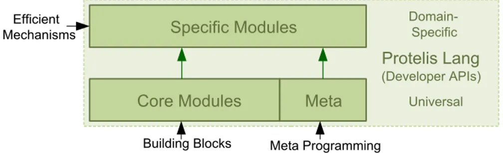
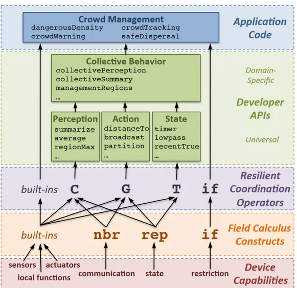
It is from this last, and particularly Proto, that field calculus and the aggregate programming approach derive, aiming at a generalisation that can effectively encompass the vast majority of the above approaches, as will be generally necessary for building complex distributed systems across a wide range of application domains. Aggregate programming is a paradigm that models large-scale adaptive systems, shifting the focus from the perspective of a single component to the whole aggregate. Its layered approach (Figure 1.1) addresses IoT (Internet of Things) systems [15] with five abstraction layers.

With a bottom-up view: (i) Each device has its own capabilities. Com-munication and device-to-device interaction are extremely heterogeneous and might require ad-hoc considerations that should not impact on the design of the aggregate. (ii) Field calculus [16] is a prominent approach to aggregate programming that addresses distributed systems as a functional composition of computational fields. Being a terse model, field calculus allows one to formally verify properties such as self-stabilisation, guaranteeing that feed-forward compositions of its constructs maintain the same properties. (iii) Core calculi are too low-level for system construction [17], allowing one to write unsafe and fragile programs. Field calculus constructs are then

com-bined into resilient2 _{coordination operators (“building block” algorithms)}

[18] leveraged to organise adaptive systems around well known coordination and state-tracking patterns. The analysis of self-organising systems suggests three basic mechanisms needed to ground complex applications: diffusion of information in the network, aggregation of distributed information, and “evaporation” of information [19]. (iv) User-friendly APIs (application pro-gramming interfaces) compose building blocks into functions which encapsu-late general complex mechanisms. (v) Application code imports APIs and built-in functions to fulfil the system requirements: an aggregate program is

3

Figure 1.1: The layered approach of aggregate computing shifts the focus from the single device perspective to a cooperative collection of devices. Software and hardware capabilities of devices are leveraged to implement aggregate-level field calculus constructs. “Building block” algorithms with provable resilience properties combine these constructs, and are further com-bined to deploy user-friendly APIs for a fully-resilient coordination of IoT systems. Adapted from [2].

a manipulation of data constructs across a region (either a discrete network or continuous space).

This dissertation contributes with the creation of protelis-lang, a new foundational library for self-organising distributed systems deployed within the Protelis framework. The Protelis language [12] implements the seman-tic of field calculus. Its highly-extensible functional approach addresses the terseness of field calculus, allowing an incremental deployment of building block algorithms and APIs for a fully-resilient coordination of distributed systems. In particular, protelis-lang captures and systematically organ-ises in a unified framework a large and heterogeneous collection of algorithms and usage patterns, including methods for common tasks such as leader elec-tion, distance estimaelec-tion, collection of distributed values, and gossip-based information dissemination.

The remainder of this dissertation is organised as follows. Chapter 2 re-views the vision of the aggregate programming paradigm and field calculus as universal approach to aggregate programming, and then provides an overview of the Protelis language for programming aggregate systems. Chapter 3 de-scribes how protelis-lang is engineered around bio-inspired patterns from [19] and their implementation as building blocks. Chapter 4 extends the workflow proposed in [20] and describes how a testing framework affects the deployment of both aggregate algorithms and protelis-lang, showing how unit testing and performance evaluation can be carried out. In Chapter 5 the efficacy and expressiveness of this library are illustrated through scenarios of large-scale pervasive computing and their empirical evaluation in simulation.

Chapter 2

Background

This section summarises the layered architecture of aggregate programming, starting with its vision and motivation. Field calculus is a universal approach to aggregate programming. Despite its universality, field calculus is still too terse to be leveraged as an actual engineering tool for complex systems. The Java-based Protelis language implements field calculus and represents a step forward to address aggregate programming challenges. New user-friendly APIs can be built leveraging Protelis, hence dramatically reducing the abstraction gap between requirements and design of aggregate systems.

2.1

Motivation

Computational entities pervade the environment, highlighting the need for new paradigms and coordination strategies to govern a collection of devices. Pervasive computing and smart cities both envision a future in which in-terconnected devices will “augment” everyday life. Infrastructural, personal and wearable “smart” devices will lead to a pervasive continuum—a dis-tributed and very dense substrate of devices—that hosts services to manage aspects of our lives. Device-to-device interaction will be context-dependent and adaptive to unexpected contingencies.

Programming and managing such complex distributed systems is chal-5

lenging and is subject of ongoing investigation in contexts such as cyberphys-ical systems, pervasive computing, robotic systems, and large-scale wireless sensor networks [21]. Distributed systems raise challenges such as robustness to faults, adaptiveness to changes in network topology and the native open-ness of pervasive scenarios. These challenges require flexible and dynamical deployment of code to devices across the network, to adaptively change its scope of execution, and to predictably integrate it with the existing services. Researchers have recognised the need of new paradigms to engineer these col-lective systems and, particularly, to coordinate complex and distributed ac-tivities [18]. Aggregate programming models distributed systems in terms of their aggregate behaviours, e.g., “distribute a dispersal signal in overcrowded areas at mass events,” and encapsulates self-organisation techniques to guar-antee a fully-resilient and robust coordination of complex services. Effective models and programming languages are needed to handle distributed systems as native aggregates of devices [16], hence diverging from a device-centric per-spective: devices are instead perceived as a single collective entity. Languages approaching aggregate programming should then provide both mechanisms for writing aggregate specifications and a global-to-local mapping to translate them into means of coordination of individual devices.

Several approaches to aggregate programming model the entire system as dynamically evolving fields [3]. Among them, field calculus is a universal approach to aggregate programming in which fields are first-class abstrac-tions leveraged to model sensors, state, and results of computation. The operational semantics of the field calculus produce a unified model support-ing self-organisation and code mobility. Fields of first-class functions allow the distribution of code by means of device interactions and higher-order calculus.

2.2. FIELD CALCULUS 7

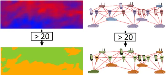
Figure 2.1: Manipulation of continuous and discrete computational fields. Fields of temperatures are transformed into boolean fields. Adapted from [22].

2.2

Field calculus

Many approaches based on computation over continuous space and time have addressed the aggregate programming challenge: [3] identifies more than 100 significant languages and models for spatial computers. Spatial computing covers a wide range of applications and biases in their approach to com-putational models. Examples of spatial computers include sensor networks, robot swarms, mobile ad-hoc networks, etc. Several of these leverage coor-dination models and languages (e.g., TOTA [23], Linda [24]) through which diffusion, recombination, and composition of information scattered in the system produce global, dynamically evolving computational fields. Formally, a computational field generalise the notion of field in physics [16]: “a com-putational field is a map from every comcom-putational device in a space to an arbitrary computational object” (Figure 2.1). Fields are aggregate-level dis-tributed data structures that gradually adapt to changes in the underlying topology and interaction with the environment. Fields can be composed to implement self-organising coordination patterns.

coordi-nation languages or models targeting aggregate programming. This “core calculus” approach captures semantics in a tiny language, expressive enough to be universal [25] yet tractable for mathematical analysis. Historically, field calculus is inspired by Proto [13]. They both express aggregate behaviour by a functional composition of operators that manipulate continuous fields and predict the behaviour of computational fields from underlying interac-tions between individual devices. These manipulainterac-tions are compiled into local rules iteratively executed in asynchronous “computation rounds:” each device receives messages from its neighbours, computes the local value of

fields, and finally spreads the result of this computation to its neighbours1_.

Both behaviour (computation and state of a device) and interaction (mes-sage content) are modelled as annotated evaluation trees. Field construction, propagation, and restriction are then supported by local evaluation “against” the evaluation trees received from neighbours.

The higher-order extension of field calculus (HFC) embeds first-class func-tions, allowing the handling of functions just like any other value. Code can be dynamically injected, moved, and executed in network domains: func-tions can be fed with other funcfunc-tions as arguments, return new funcfunc-tions, and be assigned to variables. HFC also supports anonymous functions and code migration—the functionalities being executed by a device can change over time. Together, first-class functions (what to compute) and domain-restriction (where to compute) allow predictable and safe composition of robust self-organisation mechanisms [21].

The syntax of higher-order field calculus is depicted in Figure 2.2. Five constructs are composed into programs using a Lisp-like syntax.

• Built-in function call (b e1 ... en): “point-wise” operations

involv-ing neither state nor communication. The built-in function b is applied

to its e1, ..., en input fields, and its output field maps each device

to the result of a local computation, e.g., mathematical functions (e.g.,

1_{The definition of “neighbourhood” and communication between neighbours are}

2.2. FIELD CALCULUS 9

l

::= chli | λ

;; Local value

λ ::= b | f | (fun (x) e)

;; Function value

e

::= l | x | (e e)

;; Expression

|

(

rep

x w e)

|

(

nbr

e)

|

(

if

e e e)

w

::= x | l

;; Variable or local value

F

::= (def f(x) e)

;; Function declaration

P

::= F e

;; Program

Figure 2.2: Syntax of higher order field calculus. Adapted from [21].

(add 1 2)) and context-dependent operators (e.g., (uid) returns the device UID).

• Function definition and function call: abstraction and recursion are

supported by function definition def f(x1, ..., xn) e, where xi are

formal arguments and e is the function body. (f e1 ... en) applies

f to n input fields.

• Time evolution (rep x e0 e): the “repeat” construct supports stateful

evolving fields. rep initialises the state variable x to e0, then updates it computing e against the previous value of x.

• Neighbourhood field construction (nbr e): nbr encapsules interaction between devices, and returns a field that maps each neighbouring device to its most recent available value of field e. Such “neighbouring” fields can then be manipulated and summarised with built-in *-hood oper-ators, e.g., (min-hood (nbr e)) outputs a field mapping each device to the minimum value of e amongst its neighbours.

• Domain restriction (if e0 e1 e2): branching is implemented by this

Figure 2.3: Every coordination mechanism can be expressed in field calcu-lus, but many may be difficult or impossible to express within its guaran-teed self-stabilising subset. If one coordination mechanism is asymptotically equivalent to another mechanism in the self-stabilising subset, however, then it is guaranteed to be safely composable as well. Adapted from [20].

and e2 in the restricted domain where e0 is false.

A field calculus program is then interpretable either as an aggregate-level computation on fields or as an equivalent “compiled” version automatically generated with local interaction rules. Each program consists of a set of

function definitions and a main expression eM evaluated within a network

of interconnected devices. When a device fires, it computes eM and outputs

its “value tree:,” a tree which tracks the results of the sub-expressions en-countered during the evaluation. Each evaluation on a device is performed against the most recently received value-trees of its neighbours, and the pro-duced value-tree is conversely made available to the device’s neighbours at the end of the computational round.

2.2. FIELD CALCULUS 11

2.2.1

Self-stabilising field calculus

Under fixed environmental conditions K, a network in state N is stable if no device firing changes its state. A network in state N self-stabilises to a

stable state N0 iff through a sufficiently long fair2 sequence of transitions it

necessarily reaches N0 and remains there. If the network self-stabilises to N0,

then it does so to a globally unique state that is unequivocally determined

by the environmental conditions K (namely, is independent of N ). Then, N0

can be interpreted as the output of the aggregate computation [20]. Hence, a program P is self-stabilising if its field computations react to and recover from

any change in environmental conditions, eventually reaching N0 regardless

any current state N .

In the context of an open system, self-stabilisation entails that any sub-expression of the aggregate program can be associated to a final and stable field, reached in finite time while adapting to changes in the underlying environment. This acts as the sought bridge between the sub-expressions

in program code and the emergent global outcome3 _[26].

Self-stabilisation is generally undecidable, given that computational rounds are not even guaranteed to terminate due to the universality of lo-cal computation. Thus, ensuring self-stabilisation is a matter of isolating fragments of the calculus that produce only self-stabilising field expressions. This problem has been addressed in [20] which also describes a self-stabilising sub-language of field calculus.

2.2.2

Substitution principle

Because of their generality, some coordination algorithms may not achieve good dynamic performance. More performing mechanisms exist but may be

2_{Assumption under which devices fire at almost the same frequency, assuring that no}

device is perceived as disconnected by its neighbours.

3_{While engineering a field calculus program, we can reason in terms of the field each}

expression stabilises to, rather than the expression itself. The global result is eventually a manipulation of self-stabilised fields.

difficult to express in the self-stabilising calculus (Figure 2.3).

The “substitution principle” extends the properties of self-stabilising

cal-culus: “given functions λ, λ0 with same type, λ is substitutable for λ0 iff for

any self-stabilising list of expressions e, (λ e) always self-stabilises to the

same value as (λ0 e)” [20]. Namely, two self-stabilising functions are

“sub-stitutable” if they eventually converge to the same stable state N0 when fed

with the same inputs. Indeed, as self-stabilisation does not consider the tran-sients of these functions, as long as the converged values are the same, the two functions are swappable without affecting self-stabilisation. A coordina-tion mechanism with desirable dynamic properties can replace another one, improving overall performance.

2.2.3

Resilience

Resilience is the ability to adapt to unexpected changes in working conditions [27], ensuring that the system achieves its goals in spite of certain classes of change (e.g., density of devices, perturbations). The aggregate computing framework (Figure 1.1) should provide inherent resilience: adaptation to changes is detracted from the responsibilities of an aggregate program and is demanded to the underlying layers.

Self-stabilisation guarantees resilience only to occasional disruption. Field

evolution reaches the stable state N0 only if there is enough time following

the last perturbation. However, even small perturbations to the network topology can significantly affect the result of computation.

[20, 28] propose two approaches to ensure resilience to ongoing perturba-tions: (i) the former presents an engineering methodology to replace coor-dination mechanisms with alternative and more specialised implementations that can better trade off speed with adaptiveness in certain contexts of usage (described in Chapter 4); (ii) the latter turns gossiping into a self-stabilising process by means of running parallel replicas of gossiping.

2.3. PROTELIS: AN AGGREGATE PROGRAMMING LANGUAGE 13

2.3

Protelis: an aggregate programming

lan-guage

The key idea of aggregate computing is to consider computational fields as a first-class abstraction: any computation is therefore seen as a purely func-tional transformation of fields. The computafunc-tional field calculus [29, 30] provides a universal [25] formal foundation for this approach (syntax, typ-ing, denotational and operational semantics, behaviour properties such as self-stabilisation). Being a theoretical model, any implementation of field calculus requires both an interpreter and an architecture to handle commu-nication, execution, and interfacing with external components. In addition, a framework for field calculus should be portable across both simulation en-vironments and real networked devices.

The Protelis language [12] has been developed as an implementation of field calculus similarly to the Proto VM [31]. A parser translates Protelis code into a field calculus semantics that is executed by the interpreter at regular intervals, communicating with other devices and drawing contextual information from environment variables implemented as a tuple of key-value pairs. Protelis includes the universality and self-stabilisation properties of field calculus [29] in a modern programming language with the following features [12]: (i) a functional paradigm with an imperative Java-like syn-tax, which significantly reduces barriers to adoption; (ii) full interoperability with the Java runtime and API; (iii) complete coverage of the field calcu-lus constructs; and (iv) higher-order mechanisms to enhance reusability and flexibility, and to support code mobility.

Embedding Protelis within Java ensures accessibility, portability, and ease of integration. Java reflection allows dynamic invocation of arbitrary Java code, thus allowing integration of aggregate programs with a rich existing ecosystem of libraries, devices, and applications. Still, Protelis is overall a purely functional language: a program is made of a set of function definitions (essentially, libraries formed by modules) with a main expression as starting

P ::= I F s;

;; Program

I ::=

import

m |

import

m.∗

;; Protelis/Java import

F ::=

def

f(x) {s;}

;; Function definition

s ::= e |

let

x

=

e | x

=

e

;; Statement

w ::= x | l | [w] | f | (x)->{s;}

;; Variable/Value

e ::= w

;; Expression

| b(e) | f(e) | e.

apply

(e)

;; Fun/Op Calls

| e.m(e)

;; Method Calls

|

rep

(x<-w){s;}

;; Persistent state

|

if

(e){s;}

else

{s

;}

;; Exclusive branch

|

mux

(e){s;}

else

{s

;}

;; Inclusive branch

|

nbr

{s;}

;; Neighborhood values

Figure 2.4: Protelis abstract syntax. Adapted from [12].

point of the global computation—ultimately carried on by the collection of available devices undergoing repetitive computational rounds.

The abstract syntax of Protelis is shown in Figure 2.4—overbar semi-formal notation is used to denote sequences of syntactic elements. In Pro-telis, any expression denotes a whole computational field (a space-time data structure), hence functions compute fields out of fields. Local values l (num-bers, strings, Booleans), tuples (e.g., [1, 2, "s"]), function names f, and anonymous functions ((x)->{e}), all represent “constant” fields (mapping to the same value at every device at every time). Each statement is an ex-pression to be evaluated, and a statement sequence s evaluates to the result of the last statement. Expressions are variables, values, and function calls (applied to a built-in function b, a user-defined function f, a Java method

e.m, and—byapply notation—an expression e returning a function itself).

Protelis implements the field-calculus constructs (introduced in

Sec-tion 2.2) to address space-time computaSec-tion, and adds muxas an additional

branching operator:

2.4. BUILDING BLOCKS 15 field that is initially w, and is continuously updated at each round by the unary function taking variable x and evaluating body s (e.g.,

rep(x<-0){x + 1} is the field counting computation rounds at each

device);

• nbr{e}, illustrated in Figure 2.5(b), models device-to-device interaction

and creates a field where each device maps its neighbours (including itself) to their latest available evaluation of e (such fields are then

usually reduced again with a built-in hood functions like max, min,

average, and so on, as described below);

• if(e){s;}else{s0;}, illustrated in Figure 2.5(c), performs an exclusive

branch, partitioning the network into two space-time subregions (where

e evaluates to true/false, respectively), computing s in the former

and s0 in the latter, in isolation;

• mux(e){s;}else{s0;} construct is an inclusive multiplexing branch: the

two fields obtained by computing s and s0 are superimposed, using the

former where e evaluates totrue, and the second where e evaluates to

false.

Listing 2.1 shows a composition of field calculus operators into higher-level and more user-friendly functions written in Protelis.

2.4

Building blocks

Though field calculus is a step toward practical applications, as shown in Fig-ure 1.1, its terseness makes it too low-level for programming resilient systems [17]. The “Resilient coordination” layer composes field calculus constructs in a collection of higher-level building block algorithms, simple and generalised basis elements of an “algebra” of programs with desirable resilience proper-ties [12]. Four self-stabilising algorithms (Figure 2.6) are introduced in [18] and elaborated in [20]: G (spreading), C (aggregation), T (temporary state),

H

A

A

D

H

T

H

K

B

(a) rep: time-varying field (b) nbr: field from neigh-bours

(c) if: exclusive branching

Figure 2.5: Field calculus core operators. Adapted from [17].

/* E s t i m a t i n g d i s t a n c e to a s o u r c e r e g i o n */ def d i s t a n c e T o ( s o u r c e ) { /* Time - v a r y i n g f i e l d : m i n i m u m d i s t a n c e to s o u r c e */ rep( d < - I n f i n i t y) { /* I n c l u s i v e m u l t i p l e x i n g : all d e v i c e s e v a l u a t e b o t h b r a n c h e s . * R e t u r n s 0 if s o u r c e is true , a p o s i t i v e d i s t a n c e o t h e r w i s e */ mux ( s o u r c e ) { 0 } e l s e { m i n H o o d(nbr{ d } + n b r R a n g e ) } } } /* E s t i m a t i n g d i s t a n c e to a s o u r c e r e g i o n w h i l e a v o i d i n g o b s t a c l e s */ def d i s t a n c e T o W i t h O b s t a c l e ( source , o b s t a c l e ) { /* E x c l u s i v e b r a n c h i n g : e v a l u a t e d i s t a n c e T o if o b s t a c l e is false , * e v a l u a t e I n f i n i t y o t h e r w i s e */ if ( o b s t a c l e ) { I n f i n i t y } e l s e { d i s t a n c e T o ( s o u r c e ) } }

Listing 2.1: Leveraging rep, nbr, if, mux to build higher-level and

2.4. BUILDING BLOCKS 17

(a) G: spreading (b) C: accumulation

3

1

7

2

4

3

3

1

0

(c) T: time (d) S: sparse choice

Figure 2.6: Self-organising distributed systems are often built on bio-inspired mechanisms, summarised in [19], such as diffusion and accumulation of in-formation over space and time, and symmetry breaking through mutual

inhibition. The four building-block algorithms proposed in [18] and

re-fined in [20] address these mechanisms. Their self-stabilisation and eventual consistency—adaptiveness to changes in device density, topology, etc.—have been formally proved in [20, 22], and transfer to any feed forward composition of these blocks. Reproduced from [17].

and S (symmetry breaking through mutual inhibition). Critically, any pro-gram constructed using only these operators for coordination and state (or their equivalents, per the modular proof established in [20]) is guaranteed to be self-stabilising and to have good scaling properties (though timing details of course vary depending on usage details). “Feed-forward” compositions of such algorithms are self-stabilising too. Indeed, if the input of an algorithm is stable, then its output self-stabilises as well. Any algorithm consuming its output will be fed with an input that stops changing, and eventually all algorithms will self-stabilise.

Building blocks are highly general, allowing a programmer to build and

coordinate distributed application across different applications. Each of

them captures best practises to develop flexible decentralised specifics, hid-ing the low-level details of field calculus and satisfyhid-ing three features: (i) self-stabilisation, building blocks eventually converge and, in addition, they are capable of reactively adjusting to changes in the input field and network structure; (ii) scalability to large networks; (iii) resiliency, compositions of building blocks inherit their resilient features.

2.4.1

Spreading

G, illustrated in Figure 2.6(a), produces resilient diffusion of information away from a source region, spreading this information outward along a spanning tree built applying the triangle inequality constraint, and possibly modifying that information as it spreads. In the case of multiple sources, the space is effectively partitioned into sub-regions, one per source, with each device receiving information only from its nearest source. Many functions address-ing information diffusion can be based on G, e.g., estimataddress-ing distance to one or more designated source devices and broadcasting a value from a source (Listing 2.2).

2.4. BUILDING BLOCKS 19 /* s o u r c e : f r o m w h e r e i n f o r m a t i o n is s p r e a d * i n i t : f i e l d s p r e a d f r o m s o u r c e * m e t r i c : how to e s t i m a t e d i s t a n c e * a c c u m u l a t e : how to a c c u m u l a t e i n f o r m a t i o n a s c e n d i n g a l o n g the g r a d i e n t */

def G ( source , init , metric , a c c u m u l a t e ) { rep ( d i s t a n c e V a l u e < - [I n f i n i t y, i n i t ]) { mux ( s o u r c e ) { [0 , i n i t ] } e l s e { let ndv = nbr( d i s t a n c e V a l u e ) ; m i n H o o d([ ndv . get (0) + m e t r i c .a p p l y() , a c c u m u l a t e .a p p l y( ndv . get (1) ) ]) } }. get (1) } /* D i s t a n c e to s o u r c e */ def d i s t a n c e T o ( s o u r c e ) { /* n b r R a n g e : f i e l d of d i s t a n c e s of c u r r e n t d e v i c e to its n e i g h b o u r s */ d i s t a n c e T o W i t h M e t r i c ( source , n b r R a n g e ) } def d i s t a n c e T o W i t h M e t r i c ( source , m e t r i c ) { G ( source , 0 , metric , ( v ) - > { v + m e t r i c .a p p l y() }) } /* S p r e a d v a l u e f r o m a s o u r c e */ def b r o a d c a s t ( source , v a l u e ) { G ( source , value , () - > { n b r R a n g e } , ( v ) - > { v }) }

Listing 2.2: G implementation and examples of G-related functions. Adapted from [18]. /* p o t e n t i a l : g r a d i e n t d e s c e n d e d to a g g r e g a t e i n f o r m a t i o n * a c c u m u l a t e : how to a g g r e g a t e i n f o r m a t i o n d e s c e n d i n g a l o n g the g r a d i e n t * l o c a l : l o c a l v a l u e * n u l l : n u l l v a l u e in c a s e of no n e i g h b o u r s */ def C ( p o t e n t i a l , a c c u m u l a t e , local , n u l l ) { rep ( v < - l o c a l ) { r e d u c e .a p p l y( local , h o o d( /* built - in o p e r a t o r to r e d u c e a f i e l d to a v a l u e */

( acc , e l e m e n t ) - > { r e d u c e .a p p l y( acc , e l e m e n t ) } , null ,

/* b u i l d a s p a n n i n g t r e e d e s c e n d i n g a l o n g a p o t e n t i a l */ mux (nbr( g e t P a r e n t ( p o t e n t i a l ) ) == s e l f) { nbr( v ) } e l s e { n u l l } ) ) } } /* C o u n t d e v i c e s in a g i v e n r e g i o n */ def c o u n t D e v i c e s ( s i n k ) { C ( d i s t a n c e T o ( s i n k ) , ( acc , e l e m ) - > { acc + e l e m } , 1 , 0) } /* E s t i m a t e the a v e r a g e v a l u e in a n e t w o r k */ def a v e r a g e ( sink , v a l u e ) {

C ( d i s t a n c e T o ( s i n k ) , ( acc , e l e m ) - >{ acc + e l e m } , value , 0) / c o u n t D e v i c e s ( s i n k ) }

/* S h a r e a g l o b a l a g r e e m e n t on s c a t t e r e d d a t a */

def s u m m a r i z e ( sink , a c c u m u l a t e , local , n u l l ) {

b r o a d c a s t ( sink , C ( d i s t a n c e T o ( s i n k ) , a c c u m u l a t e , local , n u l l ) ) }

Listing 2.3: C implementation and examples of C-related functions. Adapted from [18].

G: implementation details

Each device keeps track of the distanceValue which is initialised to the tuple [Infinity, init]. Its first element represents the actual shortest distance to the closest source, while the latter is the accumulated value. Devices

evaluate both branches ofmux. While the former is a point-wise expression,

the latter maps the neighbours of each device to their most recent available value of distanceValue. This value is updated applying the accumulate function to the sum of the field of distances to the closest source and the field of distances to each device’s neighbours. The resulting field is finally reduced to the tuple containing the shortest distance to the source region.

Devices in which source is true are the origins of the gradient, and return

[0, init].

2.4.2

Accumulation

C, illustrated in Figure 2.6(b) is the complement of G, addressing resilient aggregation of information across space: C is fed with what to aggregate, then performs that aggregation along a spanning tree down a potential gradient towards a source device that thus eventually reduces all the information scattered through a region into a single summary value (Listing 2.3).

C: implementation details

Each device keeps track of the value v initialised to local, and then

aggre-gates values scattered along the network. Thehoodbuilt-in function reduces

a field to a single value iteratively applying reduce to pairs of elements. acc is initialised to the first element of the field, and is updated to the result of

each aggregation. In this casehood is fed with: the reduce function, a null

value, and a field containing the latest available value of v for the neighbours

whose parent4 _{is the current device and null for the others.}

2.4. BUILDING BLOCKS 21

/* l e n g t h : t i m e p e r i o d

* z e r o : v a l u e r e p r e s e n t i n g z e r o s t a t e * d e c a y : how to d e c r e a s e t i m e

*/

def T ( length , zero , d e c a y ) { rep ( l e f t T i m e < - l e n g t h ) {

min ( length , max ( zero , d e c a y .a p p l y( l e f t T i m e ) ) ) } } /* R e t u r n t r u e o n c e e v e r y l e n g t h t i m e */ def c y c l i c T i m e r W i t h D e c a y ( length , d e c a y ) { rep ( l e f t T i m e < - l e n g t h ) { if ( l e f t T i m e == 0) { l e n g t h } e l s e { T ( length , 0 , ( t ) - > { t - d e c a y }) } } == l e n g t h }

Listing 2.4: T implementation and examples of T-related functions. Adapted from [18]. /* g r a i n : c o m p o n e n t s i z e * m e t r i c : u n i t m e a s u r e of g r a i n */ def S ( grain , m e t r i c ) { b r e a k U s i n g U i d s ( r a n d o m U i d () , grain , m e t r i c ) }

/* R e t u r n the t u p l e [ r a n d o m number , d e v i c e UID ] */

def r a n d o m U i d () { rep ( i d e n t i f i e r < - [s e l f. n e x t R a n d o m D o u b l e () , s e l f. g e t D e v i c e U I D () ]) { i d e n t i f i e r } } /* B r e a k n e t w o r k s y m m e t r y */

def b r e a k U s i n g U i d s ( uid , grain , m e t r i c ) { rep ( l e a d < - uid ) {

d i s t a n c e C o m p e t i t i o n ( d i s t a n c e T o W i t h M e t r i c ( uid == lead , m e t r i c ) , lead , uid , grain , m e t r i c )

} == uid }

/* C o m p e t e to f i n d the l e a d e r */

def d i s t a n c e C o m p e t i t i o n ( d , lead , uid , grain , m e t r i c ) { mux ( d > g r a i n ) { uid } e l s e { let thr = 0.5 * g r a i n ; mux ( d >= thr ) { [I n f i n i t y, I n f i n i t y] } e l s e { m i n H o o d( mux (nbr( d ) + m e t r i c .a p p l y() >= thr ) { [I n f i n i t y, I n f i n i t y] } e l s e { nbr( l e a d ) } ) } } }

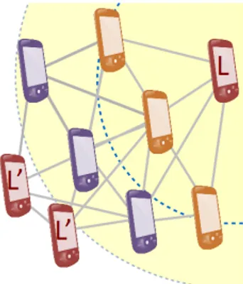
Figure 2.7: Distance competition in S from the perspective of leader L. L is the current leader of the yellow component with a grain radius. Orange devices, located within grain/2, compete with L, while purple devices, more distant than grain/2 from L, are ignored during the competition. Devices L’, more distant than grain from L, propose themselves as leaders of a new partition.

2.4.3

Time

T, illustrated in Figure 2.6(c) implements a flexible timer, which progresses from some initial state to a “zero” state at a potentially time-varying state (Listing 2.4).

T: implementation details

Each device keeps track of the leftTime value which is initialised to the length of the timer, and then returns the minimum between length and the maximum between zero and the value returned applying the decay function to the remaining time.

2.4.4

Sparse choice

S, illustrated in Figure 2.6(d), breaks symmetry through mutual inhibition, in which devices compete against others to become leaders, generating a random Voronoi partition with a characteristic grain size (Listing 2.5).

2.5. TOWARDS AN AGGREGATE LIBRARY 23 S: implementation details

Each device is identified by a tuple containing a random value and its univer-sal identifier. S breaks symmetry creating random partitions whose leaders are the devices identified by the minimum random value within a grain range. In distanceCompetition (Figure 2.7), devices compete against the others, and propose themselves as leaders in case they are farther than grain from the nearest leader. Otherwise, devices compute the minimum value of the field of leaders’ identifiers in which devices more distant than grain/2 from the closest leader are excluded from the competition (their identifiers are

replaced with the tuple [Infinity, Infinity]). breakUsingUids (hence

S) then returns true if distanceCompetition elects the current device as

a leader, false otherwise. As result, S elects a set of leaders such that no

device is more distant than grain from a leader, and no leaders are closer than grain/2.

2.5

Towards an aggregate library

The layered architecture of aggregate programming allows a hierarchical com-position of best-effort practices, encapsulating even complex coordination mechanisms in a single higher-level component (e.g., a function). Build-ing blocks represent the foundation of more complex APIs (Figure 1.1) that considerably reduce the abstraction gap between application requirements and system design. Functions such as distanceTo (Listing 2.2), average, summarize (Listing 2.3), etc., can be leveraged as higher-level “primitives” of new libraries for aggregate programming.

This approach is suitable for large-scale scenarios such as crowd applica-tions that involve people at mass public events (marathon, city festival, etc.). Personal and infrastructural devices communicate and coordinate with the others, and their opportunistic interaction smoothly supports services such as: crowd detection, crowd-aware navigation, dispersal advice, etc. A dis-tributed service is encapsulated and managed as a single function.

Program-/* E s t i m a t i n g c r o w d d e n s i t y */ def d a n g e r o u s D e n s i t y ( p , r ) { let mr = m a n a g e m e n t R e g i o n s ( r *2 , () - > { n b r R a n g e }) ; let d a n g e r = a v e r a g e ( mr , d e n s i t y E s t ( p , r ) ) > 2 . 1 7 && s u m m a r i z e ( mr , sum , 1 / p , 0) > 3 0 0 ; if( d a n g e r ) { h i g h } e l s e { low } } /* C h e c k if an a r e a has b e e n e x p o s e d at o v e r c r o w d r i s k in a g i v e n t i m e */ def c r o w d T r a c k i n g ( p , r , t ) { let c r o w d R g n = r e c e n t T r u e ( d e n s i t y E s t ( p , r ) > 1.08 , t ) ; if( c r o w d R g n ) { d a n g e r o u s D e n s i t y ( p , r ) } e l s e { n o n e }; } /* D i s s e m i n a t e w a r n i n g s i g n a l s */ def c r o w d W a r n i n g ( p , r , warn , t ) { d i s t a n c e T o ( c r o w d T r a c k i n g ( p , r , t ) == h i g h ) < w a r n }

Listing 2.6: Example of small crowd application that supports crowd

estimation and warning dissemination in Protelis. Adapted from [2].

mers compose modules to build the desired application specifying where each service should be executed and how information flows between them. For in-stance, a crowd estimation service maps information about the location of a device to a crowd density computational field. This serves as an input for crowd-aware navigation, which outputs vectors of recommended travel and warnings that are in turn an input for producing dispersal advice.

Due to the high concentration of people in constrained areas, danger-ous overcrowding issues emerge possibly leading to injuries [2]. Estimating crowd density, performing an overcrowding risk assessment and disseminat-ing warndisseminat-ings are achieved with few lines of Protelis code (Listdisseminat-ing 2.6). The proposed program is resilient and adaptive, enabling it to effectively estimate crowd density (none, low, high) and distribute warnings while executing on numerous mobile devices. Functions introduced before are composed here to show how a crowd-management library can be built on top them.

Chapter 3

Protelis-Lang library

“There is no code without project, no project without problem analysis, no problem analysis without requirements.”

Antonio Natali

In this section, we engineer protelis-lang on the bases of a multi-stage process including requirements analysis, problem analysis, and design. Out-puts from each stage are qualitatively represented in Figure 3.1.

3.1

Requirements

While a programmer may have clear ideas about the aggregate behaviours desired from a system, the details required to implement such behaviours in the low-level operations of field calculus (or their corresponding Protelis syntax) are often quite intricate and sensitive to details of their implemen-tation. This is particularly true for ensuring that behaviours are resilient and scalable, as these properties are often quite difficult to validate using either formal analysis or empirical testing [17]. In order to fulfil the promise of aggregate programming, we need a comprehensive library that provides

higher-level building blocks that are already guaranteed to be resilient and scalable, thus insulating application programmers from these challenges.

The terseness of field calculus allows a programmer to design fragile programs and requires one to “manually” address coordination and

state-tracking challenges. Building block algorithms partially reduce the

com-plexity of writing aggregate programs, still, being general functions they require specialisation. Though building blocks hide resilient best practices “under the hood,” avoiding directly use of field calculus constructs, there is a considerable gap to bridge with respect to application requirements. The protelis-lang library is located at the “Developer APIs” layer of the aggre-gate programming stack (Figure 1.1), and, as such, our work should define extensible and general core modules on which more specific ones can be built. While analysing the requirements, we highlighted three key ideas: build-ing blocks, resiliency and scalability. All of them were previously addressed in Chapter 2. As such, we defined a two-stage process to engineer our li-brary. The first challenge is defining, organising, and formalising what has already been published. In the second stage, we defined the boundaries of protelis-lang through a comparison with the state-of-art literature and fill in the missing places with respect to the existing technologies and DSLs.

3.2

Analysis

In order to construct our prototype library, we drew upon three sources in an effort to more systematically define its scope and populate its contents. At the core of the library is the system of four self-stabilising building-block operators identified in [18] and elaborated in [20]: G (spreading), C (aggre-gation), T (temporary state), and S (sparse choice). Critically, any program constructed using only these operators for coordination and state (or their equivalents) is guaranteed to be self-stabilising and to have good scaling prop-erties (though timing details of course vary depending on usage details). We then searched through all of the prior publications referenced for their

as-3.2. ANALYSIS 27 Building-Blocks Core-Modules Protelis-Lang (Developer-APIs) Universal

Specific-Modules Domain--_Specific

Efficient-Mechanisms

Meta Meta-Programming

(a) We need a comprehensive and highly extensible library providing higher-level building blocks, guaranteeing inherent resilience, and which is organised around domain-specific modules that depend on global modules (core modules and meta-programming modules). Meta Core modules Universal spreading ... accumulation ... sparsechoice ... ... time Protelis Lang (Developer APIs) meta ...

(b) Self-organising systems are built around spreading, and accumulation of in-formation over space and time [3, 19]. accumulation and sparsechoice depend on spreading as they require metrics and distance-based potentials. We added sparsechoice module for symmetry breaking.

Meta CoreFmodules Universal spreading G,FdistanceTo broadcast, dilate,F nbrRange,F... accumulation C,Fsummarize, average, countDevices,F ... FFsparsechoice S,F... T,FcyclicTimer,time cyclicFunction, limitedMemory,F ... ProtelisFLang (DeveloperFAPIs) meta boundSpreading, multiRegion, multiInstance, ...

(c) Modules are populated with building-block related functions.

Figure 3.1: Engineering the “Developer APIs” layer from Figure 1.1. We deployed the core modules of protelis-lang following three stages: (a) requirement analysis, (b) problem analysis and (c) design of protelis-lang. Green arrows depict inter-module dependencies.

protelis)

nonselfstabilizing)

lang)

state)

coord)

sparsechoice)

spreading)

accumula5on)

meta)

nonselfstabilizing)

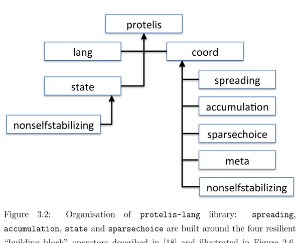
Figure 3.2: Organisation of protelis-lang library: spreading,

accumulation, state and sparsechoice are built around the four resilient “building block” operators described in [18] and illustrated in Figure 2.6, while meta contains higher-order coordination patterns and lang contains utility functions. The nonselfstabilizing sub-packages expose additional less resilient building blocks that must be applied with care for that reason.

sociated algorithms and code fragments, importing and adapting those that could be mapped onto one or more of these operators or proved equivalent, along with any other patterns and supporting functions of interest.

Finally, we compared the contents thus identified in two broad surveys: the systematic analysis of space-oriented aggregate programming languages in [3] and the analysis of biologically-inspired self-organisation patterns in [19] in order to more systematically define our scope of coverage and to identify and fill any coverage gaps that we could identify.

In particular, at this time we specifically rule out of scope of the library al-gorithms that control device movement (e.g., flocking and swarming) or that

3.2. ANALYSIS 29

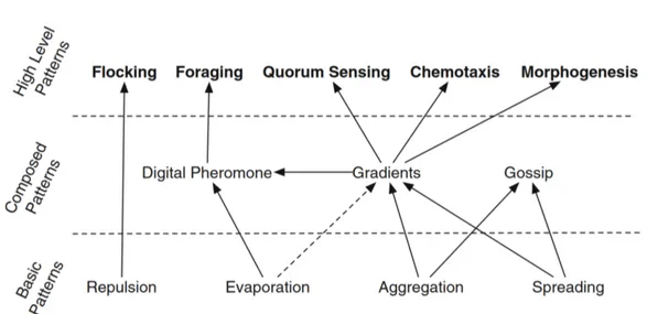
Figure 3.3: Classification of and inter-relations between bio-inspired mecha-nisms to ease the engineering of self-organising artificial systems. Adapted from [19].

work with coordinate information (e.g., localisation algorithms). Analysis of self-organisation patterns suggests three basic mechanisms needed to ground complex applications [19]: diffusion of information in the network as an ad-vertisement mechanism, aggregation of distributed information as a sensing mechanism, and “evaporation” of information as a refresh mechanism. As spreading, aggregation and evaporation are foundational mechanisms upon which more complex patterns are built (Figure 3.3), we drew parallels with G, C and T. Encouragingly, we found that the building-block operators corre-spond nicely with these three bio-inspired mechanisms.

G draws from both aggregation and spreading patterns, diffusing and ag-gregating information ascending along a gradient. G is also related to the gradient pattern as it allows diffusion of information along with the distance from the source (Listing 3.1). However, as G partitions a network of devices in “isolated” spatial sub-regions, G does not allow the aggregation of gradients propagated by different sources. Finally, G represents a possible implemen-tation of the ant foraging pattern in which the origin of the gradient and devices represent respectively nest and ants looking for food.

Both C and aggregation pattern merge, filter, and reduce information scat-tered in the system, avoiding network and memory overload. While C aggre-gates data down a potential, aggregation locally applies a fusion operator to process and synthesises macro information.

Gossip composes both aggregation and spreading patterns to eventu-ally share a global agreement about local values scattered in the system. summarize (Listing 2.3), a feed forward composition of C and G, is a possi-ble self-stabilising implementation of gossip that aggregates information in a sink and then broadcasts it back. The same composition can be leveraged to implement the quorum sensing pattern for taking collective decisions in systems where a minimum number of devices satisfying a certain condition is required.

As information might become outdated, functions should rely on more recent data. Evaporation pattern periodically reduces the relevance of data over time, and T can be leveraged to address this pattern (Listing 3.3).

The analogies between building blocks and the basic bio-inspired patterns suggest a possible organisation for our library around G, C, T, and S—though symmetry breaking is not addressed in [19], and prove that functionalities furnished by protelis-lang can potentially address a wide range of appli-cations.

3.3

Design

While software development is immune from almost all physical laws, entropy—the degree of disorder—hits hard [32]. Well-designed code consider-ably affects the productivity of system designers and programmers, especially when it comes to working with state-of-art technologies. According to Dave Thomas [33]: “Clean code can be read, and enhanced by a developer other than its original author. It has unit and acceptance tests. It has meaningful names. It provides one way rather than many ways for doing one thing. It has minimal dependencies, which are explicitly defined, and provides a clear

3.3. DESIGN 31 and minimal API.”

Testing

The three test driven development laws guarantee that minimal tests virtu-ally cover all the library code [34]. To manage testing complexity, we use Gradle as a tool for the automatic build of our library, JUnit as a testing framework, and we structured tests as follows:

• Test cases should be short and descriptive. Testing requires the creation of a new simulation environment, which we kept as simple as possible. In particular, testing an aggregate program, addressed in Chapter 4, requires the scenario configuration against which Protelis code is tested. They both cover only the strictly necessary specifications to test the desired feature;

• Every test function has one and only one concept assertion;

• Test names should be short and descriptive. Each function within the library must be tested and may require multiple unit and regression tests. In this case, test name should be a concatenation of “function name + feature being tested.”

Naming conventions

The name of a variable or a function should be as expressive as possible, explaining what it does, and how it is used. If a name requires a comment, then the name does not reveal its intent [33]. For instance, the function

definition def ebf(s) /* exponential back-off filter */ may lead to

disinformation. We prefer descriptive pronounceable names, such as def

exponentialBackoffFilter(signal). Indeed, the programmer, at first sight, can expect what the exponentialBackoffFilter function does, still, at a later stage, she should check the unit tests as they formalise the be-haviour of the function.

The Protelis language does not support types and function overload-ing. As such, we adopted internal naming conventions and introduced a

Javadoc-compliant documentation1 describing each function signature. For

instance, distanceTo (Listing 2.2) feeds G with the self.nbrRange()

met-ric. As such the field of distances returned by distanceTo strictly depends

on the back-end implementation of the Protelis ExecutionContext. We

also wanted a generic version of this function to deal with ad-hoc

met-rics. Thus we introduced a new function whose name is the

concatena-tion of “base funcconcatena-tion name + With + addiconcatena-tional parameters,” resulting in distanceToWithMetric. distanceTo then performs an inner call to the generic distanceToWithMetric that takes the desired metric as a parameter.

/* - - - F u n c t i o n s i g n a t u r e s , t y p e is d e s c r i b e d a f t e r e a c h p a r a m e t e r - - - - */ /* * * C o m p u t e d i s t a n c e to a s o u r c e . * * @ p a r a m s o u r c e bool , w h e t h e r the c u r r e n t d e v i c e is a s o u r c e * @ r e t u r n num , d i s t a n c e to the c l o s e s t s o u r c e */ def d i s t a n c e T o ( s o u r c e ) { ... } /* * * C o m p u t e d i s t a n c e to a s o u r c e . * * @ p a r a m s o u r c e bool , w h e t h e r the c u r r e n t d e v i c e is a s o u r c e * @ p a r a m m e t r i c () - > num , how to e s t i m a t e d i s t a n c e s * @ r e t u r n num , d i s t a n c e to the c l o s e s t s o u r c e */ def d i s t a n c e T o W i t h M e t r i c ( source , m e t r i c ) { ... } /* * * D i s t a n c e to n e i g h b o r s . * * @ r e t u r n num , f i e l d of d i s t a n c e s f r o m e a c h n e i g h o r */ def n b r R a n g e () { s e l f. n b r R a n g e () } /* * * Hop to n e i g h b o r s . * * @ r e t u r n num , f i e l d of ‘1 ‘ s ( hop to e a c h n e i g h o r ) */ def n b r R a n g e H o p D i s t a n c e () { 1 } /* - - - F u n c t i o n i n v o k a t i o n s - - - - */ d i s t a n c e T o ( s o u r c e ) /* d i s t a n c e b a s e d on E x e c u t i o n C o n t e x t i m p l e m e n t a t i o n */ d i s t a n c e T o W i t h M e t r i c ( source , n b r R a n g e ) /* s a m e as a b o v e */ d i s t a n c e T o W i t h M e t r i c ( source , n b r R a n g e H o p D i s t a n c e ) /* h o p s to the s o u r c e */

3.3. DESIGN 33 General but minimal API

Being a generally scoped library, protelis-lang may allow multiple solu-tions to certain problems. For instance, broadcasting the number of devices in a network:

b r o a d c a s t ( sink , c o u n t D e v i c e s ( d i s t a n c e T o ( s i n k ) ) ) ; /* b r o a d c a s t d e v i c e s */

s u m m a r i z e ( sink , sum , 1 , 0) ; /* b r o a d c a s t d e v i c e s */

Still, the core functionalities should be minimal enough to avoid redundancy. Exceptions to this rule exist in case of new functions with sensible differ-ences in the dynamic features are added to protelis-lang extending the substitution library (Chapter 4). For instance, we ended up having sev-eral substitutable functions, such as G-crfGradient-flexGradient and C-CMultiIdempotent-CMultiDivisible.

Functions as first-class abstractions

The statements within the body of a function should be all at the same level of abstraction. Mixing different levels within a function is always confusing for code readers [33]. While reading a Protelis program, the main function should be followed by those at the next level of abstraction, so that we can read the program descending one level of abstraction at a time as we read down the list of functions (step-down rule [33]).

We now consider two abstraction levels: • Field calculus constructs.

def d i s t a n c e T o ( s o u r c e ) { rep ( a c c u m u l a t o r < - I n f i n i t y) { mux ( s o u r c e ) { 0 } e l s e { m i n H o o d(s e l f. n b r R a n g e () + nbr( a c c u m u l a t o r ) ) } } }

The translation of the previous code in natural language is: distanceTo

keeps track of an accumulator initialised to Infinity. If a device is

a source, then it fires 0, otherwise it fires the minimum value of the sum of two fields: distances to its neighbours, and neighbours’ values of accumulator.

• Specialising building blocks. def sum ( sink , v a l u e ) {

C ( d i s t a n c e T o ( s i n k ) , ( a , b ) - > { a + b }) , value , 0) }

Translating this snippet into natural language is straightforward: C ac-cumulates the sum of devices’ value descending along the shortest path to the sink. This code does not include any field calculus constructs: the higher the abstraction level, the easier the explanation in natural language.

• Mixing abstraction levels.

def b r o a d c a s t S u m M i x e d A b s t r a c t i o n ( sink , v a l u e ) { rep ( a c c u m u l a t o r < - v a l u e ) {

mux( s i n k ) { sum ( sink , v a l u e ) }

e l s e { m a x H o o d P l u s S e l f(nbr( a c c u m u l a t o r ) ) } }

}

One the one hand, mixing different abstraction levels makes things hardly understandable. Each device keeps track of an accumulator initialised to value. All devices compute sum, but if a device is a sink, then it fires the actual sum, else it fires the minimum value from the field of neighbours’ accumulator.

• Same abstraction level.

def b r o a d c a s t S u m S a m e A b s t r a c t i o n ( sink , v a l u e ) { b r o a d c a s t ( sink , sum ( sink , v a l u e ) )

}

On the other hand, using the same abstraction

level dramatically simplifies the understanding of the

code. Indeed, broadcastSumSameAbstraction and

broadcastSumMixedAbstraction behave the same, but the

for-mer is easily understandable: sink devices broadcast the sum of the values accumulated in them.

Functions should avoid side effects and have a small number of arguments. Arguments are hard to test, as they increase the number of input combina-tions to be tested. Testing every combination of appropriate values can be

3.4. IMPLEMENTATION 35 daunting. When a function requires too many parameters (namely, more than three), it is likely that some of those arguments ought to be wrapped into a function or aggregated in a single value [33].

def b r o a d c a s t S u m 4 ( sink , region , o b s t a c l e , v a l u e ) { b r o a d c a s t ( sink ,

if ( r e g i o n && ! o b s t a c l e ) { sum ( sink , v a l u e ) } e l s e { 0 }

) }

def b r o a d c a s t S u m 3 ( sink , c o n d i t i o n , v a l u e ) { /* m e r g e r e g i o n and o b s t a c l e */

b r o a d c a s t ( sink , sum ( sink , if ( c o n d i t i o n ) { v a l u e } e l s e { 0 }) ) }

def b r o a d c a s t S u m ( sink , v a l u e ) { /* m e r g e c o n d i t i o n and v a l u e */

b r o a d c a s t ( sink , sum ( sink , v a l u e ) ) }

broadcastSum4 addresses two tasks: broadcasting information and filtering

obstacles and devices which are not part of region. An orthogonal2 design

promotes reuse. If functions have specific, well-defined responsibilities, they can be combined with new components in ways that were not envisioned be-fore [32]. Functions should be loosely coupled, self-contained, and with a clear scope. Modular code reduces maintenance issues, reducing development and testing, promoting reuse—the more loosely coupled the functions, the easier they are to reconfigure and reengineer, isolating “bad” code. broadcastSum3 partially optimises broadcastSum4, aggregating the two boolean parameters. However, this function is still responsible for the two tasks. broadcastSum gets rid of the filtering functionality addressing only broadcasting of a generic value.

We provided multiple versions of the same functions with an increasing generality level (again, distanceTo and distanceToWithMetric), trying to keep the numbers of parameters as small as possible.

3.4

Implementation

The layered approach of aggregate programming is suitable for engineering orthogonal systems. We composed our library as a set of cooperating

ules, each of which implements functionality independent of the others. Mod-ules are organised into universal and more specific layers, that respectively provide an increasing level of abstraction.

The result is a prototype protelis-lang library, counting more than 150 distinct functions, organised as shown in Figure 3.2. Each of the four “building block” operators is the basis for module exploiting its pattern: spreading, accumulation, sparsechoice, and time. Associated with these are nonselfstabilizing modules that collect related useful patterns that must be handled with care due to their lack of resilience. At a yet higher level of abstraction, the meta module collects general purpose patterns for combining and modulating other functions, and finally lang contains a set of simple utility and glue functions used by other modules.

The remainder of this section describes each module (except the simplistic lang) in more detail.

3.4.1

Spreading

The protelis:coord:spreading module is based around the information spreading operator G, illustrated in Figure 2.6(a). This operator produces resilient diffusion of information away from a source region, spreading this information outward along a spanning tree built applying the triangle in-equality constraint, and possibly modifying that information as it spreads. The time this takes is proportional to the diameter of the region in which G is executing.

Listing 3.1 shows example excerpts from spreading, showing how G is ex-ploited to build functions based on information moving towards the edges of a spatial region. One such example is broadcast, which spreads a copy of in-formation held by the source region. Others include distanceTo, a computa-tion of distance of every locacomputa-tion from a source region and distanceBetween, which provides every location with an estimate of the shortest distance be-tween two regions.

3.4. IMPLEMENTATION 37 applications, as the self-stabilisation rate of G is inversely bounded by the distance between the closest pair of neighbours and their communication

speed [35]. These two alternatives are more specialised but functionally

equivalent, and thus may be safely substituted for G [20]. One alternative, crfGradient [35], is a distance measure that self-repairs very rapidly but is sensitive to repeated small perturbations, while the other, flexGradient [36] is a distance measure that tolerates small distortions in return for smoother change over time.

3.4.2

Accumulation

The protelis:coord:accumulation module is based around the informa-tion accumulainforma-tion operator C, illustrated in Figure 2.6(b). This operator is the complement of G, addressing resilient aggregation of information across space: C is fed with what to aggregate, then performs that aggregation along a spanning tree down a potential gradient towards a source device that thus eventually reduces all the information scattered through a region into a single summary value. The time this takes is proportional to the diameter of the region in which C is executing.

Even small perturbations, however, can cause loss or duplication of data,

resulting in transient disruptions that impact stabilisation. Accordingly,

protelis:coord:accumulation provides alternatives to C that use multiple paths down the potential field rather than just one: as cMultiIdempotent and cMultiDivisible and their specialisations cMultiMin, cMultiSum, etc. On top of C, other functions are built that use it (and often combinations with G) to implement collective state estimation, such as summarize, which shares the result of an accumulation through a region, countDevices, which counts the number of devices in a region, and average, which estimates the average of a local value across a region (Listing 3.2).