Politecnico di Milano
School of Industrial and Information Engineering
Master of Science Degree in
Automation and Control Engineering
Adaptive control of multirotor UAVs
Master of Science Dissertation of:
Alessio Russo,
N. 838353
Advisor:
Prof. Marco Lovera
Tutors:
Ing. Davide Invernizzi
Ing. Mattia Giurato
To my family, and to whom has always believed in me.
Ringraziamenti
Questo lavoro può essere visto, da un punto di vista pratico, il riassunto di mesi di lavoro nell’apprendere un argomento nuovo, e riuscire a produrre una soluzione reale a un problema reale. Dal mio punto di vista, invece, questo lavoro è il riassunto di un percorso, nato più di 5 anni fa, grazie alla mia curiosità e al sostegno dei Professori che mi hanno sostenuto, in primis Carlo Scaglioni, Zio Lupo, il quale lo ricorderò sempre con affetto.
Questa tesi non racchiude solamente una possibile soluzione a un problema o possibili nuovi sviluppi teorici, ma contiene la passione mia e quella di tutti i Professori sotto i quali ho avuto la fortuna di studiare, i quali mi hanno trasmesso la loro voglia di cercare, provare.
Vorrei quindi ringraziare il Professor Marco lovera per l’opportunità concessami nel lavorare sull’argomento sviluppato in questa tesi, per il suo impegno e la fiducia riposta nelle mie capacità. A seguire vorrei ringraziare Davide, per avermi seguito e sopportato nonostante le mie numerose slides e le mie idee strampalate; Mattia, per il suo aiuto e la possibilità di lavorare sul quadrotore.
Vorrei ringraziare, inoltre, tutti quelli che in qualche modo mi hanno soppor-tato e mi sono rimasti vicini lungo questo difficile percorso: i miei coinquilini Dario, Gianluca e Giovanni; amici storici come Paolo, che mi hanno aiutato durante i miei momenti di difficoltà; i miei amici rimasti a Genova, fra cui Chiara, Francesca e Marcello; i miei amici con cui mi sono laureato alla laurea trien-nale: vi vorrò sempre bene nonostante le poche volte che ci vediamo. Un saluto va pure ad Alberto e agli amici di Automazione, agli amici dell’Alta Scuola Po-litecnica (Giulia, Cristina, . . . ) e il gruppo Enhances (bisogna ritornare a Berlino). Il ringraziamento più sentito va alle persone a cui voglio tanto bene, e mi scuso se lavoro un po’ troppo, però sappiate che vi penso sempre. Alice sei davvero un gioiello: sei davvero stata paziente con me, gentile e affettuosa, sono felice di averti incontrato e dedico questa tesi pure a te. I miei zii, fra cui Piera e Giovanni per farmi sentire a casa; tutti i miei cugini (scontato dire Walter? :) ) e parenti. Infine, dedico questa tesi pure ai miei nonni, che hanno creduto in me e volutob ene: sò che leggerete queste righe in qualche modo, sappiate che ce l’ho fatta. A Demy, Katy, Rudy e mia Mamma: nonostante la distanza siete sempre vicini al mio cuore. Grazie,
Abstract
This thesis tackles the problem of describing the current State of the Art regarding Adaptive Control, and, based on that knowledge, conceive a preliminary solution to adaptively control the attitude of a quadrotor vehicle, which already has a baseline controller, in case of damages or undesired events.
The work needed to come up with a solution gave birth to a new type of adaptive control scheme: in fact in literature baseline controllers are tuned so that they are included inside the adaptive controller, which is not always feasible.
First and foremost a brief overview of the UAVs is given. It is followed by a review of the literature regarding adaptive control of continuous systems. This was necessary since adaptive control is a highly fragmented topic. In particular, first are presented basic theorems that are the fundamentals bricks of Adaptive Control Theory.
The following part of the thesis is mainly theoretical: in this part new results and theorems are developed in order in order to make a preliminary theory necessary to design adaptive schemes with adaptive controllers that do not integrate the baseline controller. The theory is given for both the MRAC controller and the L1 adaptive controller, with annexed examples to show the use of the theory
developed.
The last part of thesis makes use of the theory developed in the first part to cope with the original problem of augmenting the baseline controller of an existing quadrotor with an adaptive controller. Various adaptive control schemes are presented, showing the pro and cons of each one.
Of the presented schemes the augmented L1 adaptive controller was chosen to be
tested on the simulator of the complete model of the quadrotor, which includes sensor’s noise, displaying the same performances of the simulations done before-hand. Further, that model was chosen to be tested on the real quadrotor.
Results show that by using an adaptive controller in conjunction with a nominal controller there is an increased tracking performance in case of actuator failure or external disturbance, with an increased velocity of response of about 2 ÷ 3 times the one exhibited by the baseline controller. Finally, few experimental tests were carried out using the L1 adaptive control scheme, which confirmed an increase of
the tracking performance.
Lastly, the appendix presents the Adaptive Control Library: a library devel-oped during the course of this work, in Simulink, that implements various tools helpful to develop robust adaptive control schemes.
Sommario
Il progetto di questa tesi è nato con l’idea di estendere il controllo nominale d’assetto di un veicolo quadricottero, composto da due regolatori PID in cascata tarati attraverso la tecnica H∞, con un controllo adattativo, capace di far fronte a
incertezze e disturbi che possano rendere la dinamica del quadricottero instabile. Nella letteratura questo problema, visto da un punto di vista generico e non specifico al veicolo quadricottero, è di per sè un nuovo argomento: infatti solita-mente gli schemi di controllo adattativi vengono sintetizzati includendo il controllo nominale all’interno dell’algoritmo adattativo, il cui controllo nominale è solita-mente un controllo proporzionale e/o al più integrativo.
Oltre al problema di dover affrontare un nuovo tipo di design, c’è il problema che i sistemi di controllo adattativi sono altamente suscettibili a dinamiche non modellate e a disturbi che non si possono cancellare direttamente all’input del sistema (anche dette incertezze unmatched): questo porta a un’ulteriore difficoltà nel sintetizzare un sistema di controllo utilizzabile poi realmente. Le difficoltà risultano amplificate poi nel caso di evidenti ritardi di comunicazione nel canale di controllo o rumore/ritardi sui sensori. Questo è particolarmente vero nel caso del veicolo quadricottero utilizzato, essendo un veicolo sviluppato recentemente. Tutto ciò ha portato a dover fare una revisione dello stato dell’arte riguardo il controllo adattativo, la quale è illustrata come prima parte teorica di questo lavoro. Gli argomenti ivi presentati sono essenziali per poter comprendere le basi del controllo adattativo e le varie modifiche conosciute allo stato dell’arte che pos-sono aiutare nel sintetizzare uno schema di controllo robusto ai disturbi. Inoltre, viene presentata la recente tecnica del controllo L1 adattativo, la quale garantisce
robustezza e velocità di adattazione grazie alla sua struttura. In questa prima parte viene fornito un ulteriore contributo di tipo personale, basato sull’esperienza maturata nello studiare questa tecniche, e viene dimostrata una nuova condizione sufficiente di stabilità per il controllo L1, meno conservativa rispetto a quella
presentata dai suoi autori.
Successivamente, in base alla teoria sviluppata nella prima parte, si è potuto creare un nuovo tipo di architettura di controllo adattativo che permette di risolvere il problema di estendere un controllo nominale. Tale architettura si basa sul fatto che viene fatto uso di un osservatore, sia ad anello aperto o chiuso, il quale non ha bisogno di sapere quale sia la struttura del controllo nominale. L’idea di fondo è di realizzare un controllo tale che l’errore della dinamica fra l’impianto e l’osservatore diminuisca nel tempo.
viii
Questa tecnica è in contrasto con gli schemi adattativi usati fino ad ora: infatti solitamente negli schemi diretti si fa uso di un modello di riferimento, men-tre negli schemi indiretti si fa uso di un identificatore o predittore. Attraverso questi schemi di riferimento viene poi costruito un errore fra lo stato dell’impianto e lo stato del modello di riferimento che permette di identificare i parametri incerti. Grazie alla struttura dell’osservatore, la tecnica sviluppata in questo lavoro permette di estendere qualsiasi controllo nominale, previa qualche assunzione, con un controllo adattativo, il quale non deve conoscere alcunchè riguardo la struttura del controllo nominale né ne modifica la struttura.
Nell’ultima parte della tesi è mostrato il design di vari schemi di controllo adattativi e le loro performance. Inizialmente vengono brevemente introdotte le conosciute equazioni che descrivono la dinamica di un veicolo quadricottero. Successivamente l’architettura e la robustezza del controllo nominale vengono presentate, in con-giunzione con la stima dei parametri incerti del sistema e il loro possibile insieme di appartenenza.
In base a questa descrizione nominale e incerta del sistema vengono sintetizzati diversi schemi adattativi, di cui i più importanti sono stati inclusi in questo lavoro, in base alla teoria sviluppata in precedenza.
Vengono poi mostrati i risultati di simulazione sul controllo d’assetto di un singolo asse, includendo metriche riguardo le performance del controllo e una breve comparazione dei vari metodi. È inoltre stato effettuato un test sul simu-latore reale usato per per simulare il modello completo del quadricottero: nella simulazione è stato implementato un controllo adattivo completo per i tre assi e viene presentato un video riguardo l’esito della simulazione.
Alla fine del capitolo viene sviluppata un nuovo controllo nominale basato sulla tecnica del backstepping, successivamente estesa con un controllo adattivo, per poter verificare le performance con un controllo nominale diverso da quello usato in precedenza.
Il capitolo finale di questa parte mostra alcuni brevi test eseguiti sul quadri-cottero reale, svolti alla fine del lavoro. Questi test, svolti usando il controllo adattativo L1 , mostrano una miglioria nell’inseguire il riferimento in caso di
disturbi o nonlinearità.
Nelle conclusioni vengono presentate varie nuove idee che potrebbero risultare in nuovi risultati teorici e pratici. Infine, nell’appendice, oltre a mostrare risul-tati matematici utilizzati nella tesi, viene presentata l’Adaptive Library Toolbox, una libreria Simulink sviluppata durante il lavoro di questa tesi che permette di implementare schemi adattativi rapidamente ed efficacemente.
Contents
Nomenclature xxiv
I
Introduction
1
1 Overview of the content 3
2 Unmanned Aerial Vehicles and Quadrotors: State-of-Art and
Literature Survey 7
2.1 Field of use . . . 9
2.2 Impact of Drones on Society and Developments . . . 11
2.3 Adaptive Control of Quadrotors . . . 16
2.3.1 MRAC Schemes . . . 16
2.3.2 L1 Adaptive Control Schemes . . . 19
II
Adaptive Control: State-of-Art
21
3 Introduction to Adaptive Control 23 3.1 Short history of Adaptive Control . . . 243.2 Adaptive Schemes . . . 26
3.3 Adaptive Laws . . . 27
3.3.1 Sensitivity methods . . . 27
3.3.2 Gradient and Least-Squares methods . . . 28
3.3.3 Lyapunov design and stability of non autonomous systems 30 4 Model Reference Adaptive Control 35 4.1 Introduction . . . 35
4.1.1 Reference model and command tracking problem . . . 36
4.1.2 Problem formulation and plant model . . . 37
4.2 Direct approach . . . 39
4.2.1 Problem formulation . . . 39
4.2.2 Scheme analysis . . . 39
4.2.3 Stability analysis and adaptive laws derivation . . . 40 xi
xii Contents
4.3 Indirect approach . . . 42
4.3.1 Problem formulation . . . 42
4.3.2 Scheme analysis . . . 43
4.3.3 Stability analysis and adaptive laws derivation . . . 43
4.4 Combined/Composite MRAC . . . 45
4.4.1 Problem formulation . . . 45
4.4.2 Indirect adaptation with filtered dynamics . . . 46
4.4.3 Composite adaptation . . . 47
5 Neural Networks in Adaptive Control 49 5.1 Sigmoidal Feedforward Neural Networks . . . 50
5.2 Feedforward RBF Neural Networks . . . 51
5.3 Approximation of State Nonlinearities . . . 53
6 Robust Adaptive Control 55 6.1 Introduction . . . 55
6.1.1 Parameter drift . . . 56
6.2 Adaptive law robustness modifications . . . 59
6.2.1 Dead-zone modification . . . 59 6.2.2 σ-modification . . . . 60 6.2.3 e-modification . . . . 61 6.2.4 Optimal modification . . . 62 6.2.5 Projection Operator . . . 63 6.2.6 K -modification . . . . 66 6.2.7 Q-modification . . . . 67 6.2.8 Derivative-free modification . . . 68
6.2.9 Loop-transfer recovery modification . . . 69
6.2.10 Concurrent learning modification . . . 70
6.3 Adaptive gain modifications . . . 73
6.3.1 Kalman filter modification . . . 73
6.3.2 Covariance adaptive gain with forgetting factor modification 74 6.4 Adaptation in case of unknown actuator structure . . . 75
6.4.1 Hedging-signal augmentation . . . 76
6.4.2 Pseudo-Control Hedging . . . 78
6.5 Adaptive Control law in case of time delays . . . 78
6.6 Closed Loop Reference Models . . . 80
6.6.1 Performance . . . 82
6.7 Unmatched uncertainties and Adaptive Backstepping . . . 84
7 L1 Adaptive Control 85 7.1 Introduction . . . 85
7.2 L1 Basic Control Scheme with Uncertain Input Gain . . . 88
Contents xiii
7.2.2 Control Architecture . . . 88
7.2.3 Analysis of the Closed-Loop System . . . 92
7.2.4 Design of the L1 Adaptive Controller . . . 96
7.2.5 Extension to systems with Unmodeled Actuator Dynamics 98 7.3 L1 Piecewise Constant Scheme . . . 100
7.3.1 Problem formulation . . . 100
7.3.2 Control Architecture . . . 102
III
Adaptive Augmentation of a Baseline Controller 109
8 Adaptive Augmentation: introduction and problem formulation111 8.1 Nominal model . . . 1138.2 Uncertain model . . . 117
8.2.1 Uncertain actuator . . . 117
9 MRAC Augmentation Design 119 9.1 Observer Like Reference Model . . . 119
9.2 Control law . . . 120
9.3 Stability Analysis and Adaptive Laws . . . 121
9.4 Extension to System with unmeasured Actuator Dynamics . . . . 123
9.5 Example: Aircraft Short-Period Dynamics and Control . . . 124
9.5.1 Pulse wave response . . . 128
9.5.2 Sinusoidal response . . . 130
10 Basic L1 Augmentation Design 133 10.1 Observer Like Predictor Model . . . 133
10.2 Control Law . . . 134
10.3 Stability Analysis and Adaptive Laws . . . 134
10.4 Stability of the reference model . . . 135
10.5 Extension to System with Unmodeled Actuator Dynamics . . . . 137
10.6 Example: Aircraft Short-Period Dynamics and Control . . . 139
10.6.1 Pulse wave response - K = 55 . . . 141
10.6.2 Pulse wave response - K = 300 . . . 142
10.6.3 Pulse wave response - K = 103 . . . 143
IV
Dynamics and Control of a Quadrotor Helicopter 145
11 Dynamics of a Quadrotor Helicopter 147 11.1 Earth and Body Axes . . . 14711.1.1 Euler angles . . . 147
11.2 Kinematics and Flight Dynamics . . . 149
xiv Contents
11.2.2 Angular Motion . . . 149
11.2.3 External Forces and Moments . . . 151
11.2.4 Mixer Matrix . . . 152
11.2.5 Actuator model . . . 153
12 System Analysis and Nominal Behaviour 155 12.1 Uncertainties analysis . . . 155
12.1.1 Parameters uncertainties . . . 155
12.1.2 Control moment uncertainties . . . 159
12.1.3 External disturbances . . . 161
12.1.4 Complete model with uncertainties . . . 161
12.2 Nominal Controllers . . . 163
12.3 Robustness analysis . . . 166
12.3.1 Introduction and Definitions . . . 166
12.3.2 Nominal System Robustness . . . 168
12.3.3 Uncertain System Robustness . . . 172
12.4 Simulations . . . 175
12.4.1 Step response: nominal conditions . . . 178
12.4.2 Step response: worst case conditions . . . 179
12.4.3 Load disturbance in worst case conditions . . . 180
12.4.4 Reduction of control effectiveness in worst case conditions 182 13 Adaptive Control Augmentation: analysis and design 185 13.1 Baseline controller and assumptions . . . 186
13.2 MRAC Design . . . 187
13.2.1 Plant model . . . 187
13.2.2 Control law . . . 188
13.2.3 Observer like reference model and error dynamics . . . 188
13.2.4 Adaptive laws . . . 189
13.2.5 Simulations and Time Delay Margin Analysis . . . 192
13.3 L1 Adaptive Control Design . . . 198
13.3.1 Plant model . . . 198
13.3.2 Design of the filter C(s) . . . 198
13.3.3 Observer like predictor model and Control law . . . 201
13.3.4 Adaptive laws . . . 201
13.3.5 Simulations and Time Delay Margin Analysis . . . 202
13.4 L1 Adaptive Control - Implementation on the quadrotor simulator 208 13.4.1 Implementation . . . 208
13.4.2 Simulations . . . 213
13.5 L1 Adaptive Control design - Piecewise Constant Adaptive Law . 219 13.5.1 Plant model . . . 219
13.5.2 Observer like predictor model and Control law . . . 219
Contents xv
13.5.4 Simulations and Time Delay Margin Analysis . . . 221
13.6 Overall performance analysis . . . 227
13.7 L1 Backstepping Adaptive Control . . . 229
13.7.1 Backstepping design . . . 229
13.7.2 Simulations and Time Delay Margin Analysis . . . 231
13.7.3 L1 Adaptive Backstepping design . . . 234
13.7.4 Simulations and Time Delay Margin Analysis . . . 236
14 Adaptive Control: experimental results 241 14.1 Introduction . . . 241
14.2 Experimental results . . . 242
14.2.1 Experiments design . . . 242
14.2.2 Adaptive Control design . . . 244
14.2.3 Results . . . 245
V
Conclusions
251
15 Conclusions 253 15.1 Analysis of the work . . . 25315.2 Future work . . . 254
VI
Appendix
257
16 Adaptive Control Library 259 16.1 Adaptive Control Library . . . 25917 Mathematical appendix 263 17.1 Lp spaces and Input-Output Stability . . . 263
17.2 Approximate Mean And Variance of bivariate Random Variables . 268 17.2.1 Approximate mean derivation . . . 268
17.2.2 Approximate variance derivation . . . 269
17.3 Persistency of Excitation . . . 270
17.4 L1 norm bound of a transfer function . . . 272
List of Figures
2.1 Examples of UAVs. . . 9
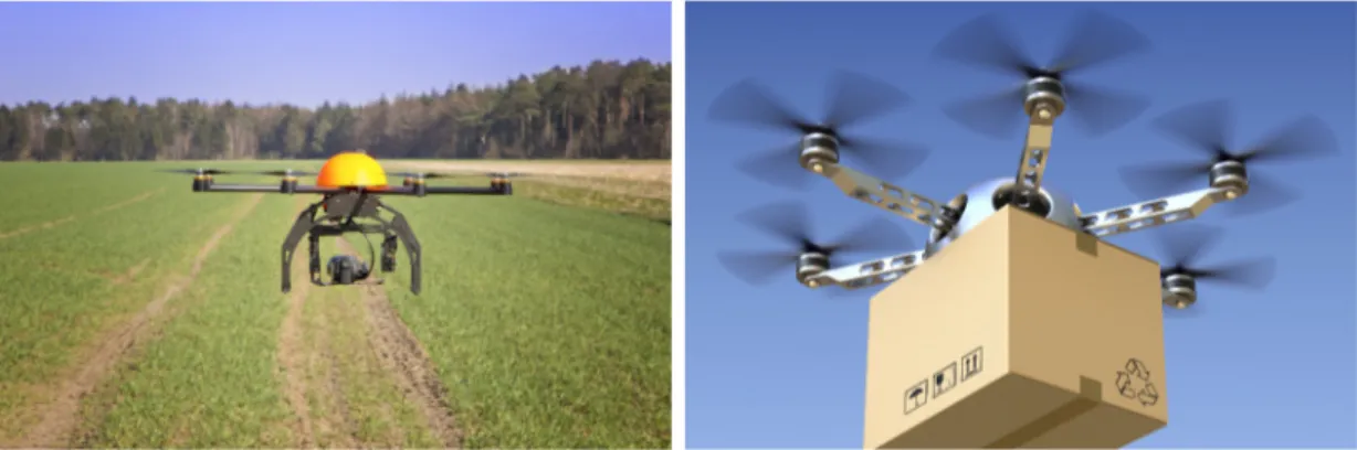
2.2 Field monitoring drone and delivery drone. . . 10
2.3 DoD Unmanned Systems Funding from 2014 to 2018. . . 11
2.4 Economic Impact from UAV Industry on the US Market. . . 12
2.5 UAV Research and Development by country. . . 13
2.6 UAV and Quadrotor number of articles indexed per year by Google Scholar. . . 13
2.7 Adoption Curve and Hype Curve regarding the Drone Market. . . 15
3.1 North American Aviation X-15A-3 56-6672 over Delamar Lake, Nevada (U.S. Air Force). . . 24
3.2 Crushed forward fuselage of North American Aviation X-15A-3 56-6672 (NASA). . . 25
3.3 UUB Concept for nonautonomous systems. . . 32
4.1 Direct Model Reference Adaptive Control scheme. . . 39
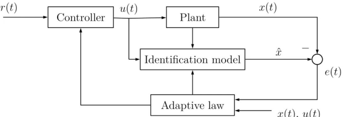
4.2 Indirect Model Reference Adaptive Control scheme. . . 42
4.3 Combined/Composite Model Reference Adaptive Control scheme. 45 5.1 Single-hidden-layer feedforward NN with N neurons. . . . 50
6.1 Unmatched uncertainty example: plot of (e, ∆Θ). . . . 57
6.2 Unmatched uncertainty example: plot of the estimates. . . 58
6.3 Unmatched uncertainty example: plot of the plant states. . . 58
6.4 Projection Operator illustration. . . 64
6.5 Modified Direct MRAC Scheme. . . 80
7.1 Direct MRAC scheme with a low-pass filter C(s). . . . 86
7.2 L1 adaptive control scheme with a low-pass filter C(s). . . . 87
7.3 L1 adaptive control architecture. . . 92
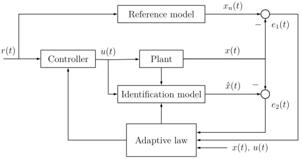
8.1 Adaptive augmentation scheme . . . 111
8.2 Observer model used to augmented a baseline controller. . . 115
9.1 Aircraft Short Period motion . . . 124 xvii
xviii List of Figures 9.2 Augmented MRAC example: simulation with pulse-wave input, 1. 128 9.3 Augmented MRAC example: simulation with pulse-wave input, 2. 129
9.4 Augmented MRAC example: simulation with sine-wave input, 1. . 130
9.5 Augmented MRAC example: simulation with pulse-wave input, 2. 131 10.1 Analysis of kGd(s)kL1 for Λ ∈ ∆λ, θ= [−50, −50]. . . 139
10.2 Analysis of kGd(s)kL1 for Λ = 0.5, θ = [7.5Mα,2.5Mq]. . . 140
10.3 Simulation of the L1 adaptive controller for K = 55. . . 141
10.4 Simulation of the L1 adaptive controller for K = 300. . . 142
10.5 Simulation of the L1 adaptive controller for K = 103. . . 143
11.1 Quadcopter configuration. . . 151
12.1 Inner loop controller . . . 164
12.2 Outer loop controller . . . 164
12.3 Inner loops Bode Diagrams. . . 169
12.4 Outer loops Bode Diagrams. . . 171
12.5 Simulink Attitude Scheme . . . 177
12.6 Y Axis: step response in nominal conditions . . . 178
12.7 Y Axis: step response in the worse case conditions . . . 179
12.8 Y Axis: load disturbance in worst case conditions. . . 180
12.9 Y Axis: loss of control effectiveness in worst case conditions. . . . 182
13.1 Simulink Attitude Scheme - MRAC . . . 191
13.2 MRAC - Simulation - Load Disturbance 1. . . 192
13.3 MRAC - Simulation - Load Disturbance 2. . . 193
13.4 MRAC - Simulation - Loss of Control Effectiveness 1. . . 195
13.5 MRAC - Simulation - Loss of Control Effectiveness 2. . . 196
13.6 L1 Adaptive control: design of C(s) - L1 norm of Gd(s)G1(s) . . . 200
13.7 L1 - Simulation - Load Disturbance 1. . . 202
13.8 L1 - Simulation - Load Disturbance 2. . . 203
13.9 L1 - Simulation - Loss of Control Effectiveness 1. . . 205
13.10L1 - Simulation - Loss of Control Effectiveness 2. . . 206
13.11Simulink Scheme - Quadrotor Simulator - Top view . . . 209
13.12Simulink Scheme - Quadrotor Simulator - Attitude Controller . . 210
13.13Simulink Scheme - Quadrotor Simulator - L1 Controller . . . 210
13.14Simulink Scheme - Quadrotor Simulator - L1 Controller single axis 211 13.15Simulink Scheme - Quadrotor Simulator - L1 Controller - Observer and Estimator Blocks . . . 212
13.16Simulink Scheme - Quadrotor Simulator - L1 Controller - Estimator213 13.17L1 - Simulation - Loss of Control Effectiveness - Position . . . 215
13.18L1 - Simulation - Loss of Control Effectiveness - Control . . . 216
13.19L1 - Simulation - Loss of Control Effectiveness - Estimates . . . . 217
List of Figures xix
13.21L1 piecewise Constant- Simulation - Load Disturbance 1. . . 221
13.22L1 piecewise constant - Simulation - Load Disturbance 2. . . 222
13.23L1 piecewise constant - Simulation - Loss of Control Effectiveness 1.224 13.24L1 piecewise constant - Simulation - Loss of Control Effectiveness 2.225 13.25Adaptive control schemes performance improvement. . . 228
13.26Y Axis, backstepping control: load disturbance. . . 231
13.27Y Axis, backstepping control: loss of control effectiveness. . . 232
13.28Backstepping time delay margin . . . 233
13.29L1 Backstepping Adaptive control: design of C(s) - L1 norm of Gd(s)235 13.30Y Axis, L1 piecewise constant adaptive backstepping: load distur-bance, 1. . . 236
13.31Y Axis, L1 piecewise constant adaptive backstepping: load distur-bance, 2. . . 237
13.32Y Axis, L1piecewise constant adaptive backstepping: loss of control effectiveness, 1. . . 238
13.33Y Axis, L1piecewise constant adaptive backstepping: loss of control effectiveness, 2. . . 239
13.34Y Axis, L1 piecewise constant adaptive backstepping: time delay margin. . . 240
14.1 Quadrotor used for the tests. . . 242
14.2 Loss of thrust γ2 due to the disturbance d in hovering conditions. 244 14.3 Experimental results: steady state control - pitch angle . . . 245
14.4 Experimental results: steady state control - control signal M. . . 246
14.5 Experimental results: pulse wave step reference command - pitch angle. . . 248
14.6 Experimental results: pulse wave step reference command - control signal M. . . 248
List of Tables
6.1 Common instability causes happening in adaptive control schemes. 56 12.1 Normal distribution parameters for A, I . . . 156 12.2 Rates controllers parameters. . . 164 12.3 Angular controllers parameters. . . 165 12.4 Margins of the inner loops in nominal conditions. . . 168 12.5 Margins of the outer loops in nominal conditions. . . 170 12.6 X, Y Axes: margins of the inner loops in uncertain conditions. . . 172 12.7 X, Y Axes: margins of the outer loops in uncertain conditions. . . 173 12.8 X, Y inner loops: parameters for which we have low φm and gm. . 173 12.9 X, Y outer loops: parameters for which we have low φm and gm. . 173 12.10Z Axis: margins of the inner loop in uncertain conditions. . . 174 12.11Z Axis: margins of the outer loop in uncertain conditions. . . 174 12.12Z inner loop: parameters for which we have low φm and gm. . . . 174 12.13Z outer loop: parameters for which we have low φm and gm. . . . 174 13.1 MRAC - Load disturbance: Performance improvements . . . 194 13.2 MRAC - Loss of control effectiveness: Performance improvements 197 13.3 MRAC Time Delay Margin . . . 197 13.4 L1 - Load disturbance: Performance improvements . . . 204
13.5 L1 - Loss of control effectiveness: Performance improvements . . . 207
13.6 L1 Time Delay Margin . . . 207
13.7 L1piecewise constant - Load disturbance: Performance improvements.223
13.8 L1 piecewise constant - Loss of control effectiveness: Performance
improvements . . . 226 13.9 L1 piecewise constant Time Delay Margin . . . 226
13.10Adaptive control schemes performance: load disturbance. . . 227 13.11Adaptive control schemes performance: loss of control effectiveness. 227 13.12Adaptive control schemes performance: time delay margin
compar-ison. . . 228 16.1 Adaptive library blocks description. . . 261
xxiv Nomenclature
Nomenclature
Acronyms
UUB Uniform Ultimate Boundedness
AC Adaptive Control
MRAC Model Reference Adaptive Control
CMRAC Composite/Combined MRAC
L1 L1 Adaptive Control
NN Neural Network
RBF Radial Basis Function
KF Kalman Filter
CRM Closed Loop Reference Model
RHP Right Half Plane
LHP Left Half Plane
iff if, and only if
Number Sets R Real numbers C Complex numbers Physics constant g Gravitational constant Other symbols Lp Space of functions Lp
ub Baseline (or nominal) control signal
ua Adaptive control signal
ON ED North-East-Down coordinate system
ae Angles vector described in the ON ED reference
ωb Euler rates
In Inertia tensor
xxv
Notation
k · k if not specified, euclidean norm
k · kLp Lp norm
ˆ· Estimated value
˜· Parameter error
λ(A) Set of eigenvalues of the real squared matrix A λmin(A) Minimum eigenvalue of the real squared matrix A
Part I
Introduction
“Begin at the beginning," the King said gravely, “and go on till you come to the end: then stop." —Lewis Carroll, Alice in Wonderland
Chapter 1
Overview of the content
This thesis tackles the problem of describing the current State of the Art regarding Adaptive Control, and, based on that knowledge, conceive a preliminary solution to adaptively control a Quadrotor vehicle, which already has a baseline controller, in case of damages or undesired events. This is, in fact, a new kind of problem: in literature baseline controllers are tuned so that they are included inside the adaptive controller, whilst the objective of this thesis is to develop an adaptive controller capable of adapting without necessarily having the knowledge of the baseline controller architecture.
Successively the theory developed to augment a baseline controller will be used to adaptively control a quadrotor vehicle. Multirotor vehicles and UAVs are of high interest in nonlinear control theory: they are highly suited to be equipped with nonlinear controllers capable of cancelling disturbances and nonlinearities. Fur-ther, the human is inherently not able to control the fast dynamics of a quadrotor, hence they are a suitable test bed for linear and nonlinear controllers.
At the beginning of this thesis a brief overview of the UAVs market nowadays and their possible field of use is given. The last section of part I describes the main adaptive control schemes used to control UAVs at the current state of the art. Next, in part II, a literature review of adaptive control of continuous systems is given. This was necessary since adaptive control is a highly fragmented topic. In particular, first are presented basic theorems that are the fundamentals bricks of Adaptive Control Theory. Next, is shown the basic framework we are interested in and Model Reference Adaptive Control (MRAC).
Successively, Robust Adaptive Control Theory is introduced, which brings a list of tools that can help the controller when designing an adaptive scheme in presence of unmatched uncertainties and disturbances.
Finally, at the end of this part, the L1 adaptive control, which is a new kind of
4 Chapter 1: Overview of the content technique, is presented. Throughout all the methods presented in this part some personal comments were written regarding the theory.
The third part of the thesis is mainly theoretical: in this part new results and theorems are developed in order in order to make a preliminary theory necessary to design adaptive schemes with adaptive controllers that do not integrate the baseline controller. The theory is given for both the MRAC controller and the L1
adaptive controller.
The conceivement of a new theory was necessary in order to cope with the problem of augmenting a baseline controller, simple or complex, with an adaptive controller flawlessly. This theory is based on the fact that an observer is used, and the control is designed so that it tries to match the plant output with the observer output. This is different from the methods that have been used up to now: in fact the two main models used in adaptive control are the reference model and the identifier model. The former defines the desired reference dynamics, whilst the latter tries to identify the real plant. The scheme developed in this thesis is different because of the fact that a different problem was faced: the augmentation of a baseline controller.
The fourth part of thesis deals with the problem of augmenting the baseline control of an existing quadrotor with an adaptive controller. First is explained the dynamics of the quadrotor and the architecture of the nominal controller. Next, the robustness of the system in case of uncertainties or damages, such as loss of control effectiveness or a load disturbance, is analysed.
Based on that, various adaptive control schemes are presented, showing the pro and cons of each one. Of the presented schemes the augmented L1 adaptive
controller was chosen to be tested on the simulator of the complete model of the quadrotor, including sensor’s noise, displaying the same performances of the simulations done beforehand. Further, that model was chosen to be tested on the real quadrotor, whose results are described in the last chapter of Part III. At the end of Part III is also shown a different nominal controller, designed using backstepping, augmented with an L1 piecewise constant adaptive controller.
Finally, the last part of the thesis, the appendix, presents the Adaptive Control Library: a library developed during the course of this work, in Simulink, that implements various tools helpful to develop robust adaptive control schemes. After, some mathematical tools that were necessary to develop the theory of this thesis, are presented.
It should be noted that various theorems were derived during the work of this thesis: all of them are presented in part II and III. In particular, in part 6 other
5 than personal considerations, is shown how to translate the projection operator set to a set with centre different than 0. In chapter 7 is given the proof for a new stability condition of the L1 controller, less conservative than the one given in
[30]. Finally, in chapters 8, 9, 10 are presented the theorems for augmenting a baseline controller with an adaptive controller.
Chapter 2
Unmanned Aerial Vehicles and
Quadrotors: State-of-Art and
Literature Survey
Nowadays we are witnessing the birth of a new type of aircraft: UAV, which is an acronym for Unmanned Aerial Vehicle. UAVs are also referred to as drones, and are a particular type of aircraft with no pilot on board. UAVs can be remote controlled aircraft (e.g. , flown by a pilot at a ground control station) or can fly autonomously based on pre-programmed flight plans or more complex dynamic automation systems.
The origin of drones can be traced back to the middle of the 19th century when the Austrian military attacked the enemy Italian city of Venice using balloons laden with explosives, but being entirely at the whim of the wind, a dangerously unpredictable flight-path saw many explode over Austrian territory. In 1898, inventor Nikola Tesla displayed a small unmanned boat that appears to change direction on verbal command. He used RF to change the course of the boat. In 1915, he gave a dissertation on using armed pilotless aircraft capable of defending the US. Drones similar to the ones used today started showing during the Second World War.
Commonly there are two types of UAVs: multirotor and fixed-wing vehicles. The latter makes use of the same principles of airplanes; it needs a launching ramp to take off (and a flat area to safely land) and the wings produce the force necessary to lift the drone. The multirotor design resembles the working principle of helicopters; the configuration of the rotors determines the stability and precision of manoeuvres it can perform in the air. A type of multirotor is the quadrotor: it can be described as a UAV lifted and directed by four rotors. The fact that a quadrotor attains its lift from its rotors leads to its classification as rotorcraft. As opposed to most helicopters, propeller blades of quadrocopters, in general, are
8 Chapter 2: UAV and Quadrotors: State of Art not pitch-varying. The control of the motion is achieved by adjusting the angular speed of each rotor which, in turn, changes the thrust and torque generation, and thus attitude in desired directions.
Both fixed-wing and multirotors are provided with an onboard computer which has many tasks as controlling the stability, allowing radio-commanding, retrieving data from sensors.
The two designs are easy to compare: the multirotor is able to take-off and land vertically, and is therefore best suited for harsh environments that are not easily accessible. On the other hand, whilst fixed-wing UAVs are best suited for long flights, the multirotor has poorer battery life, which limits its range of action and the distance covered.
The onboard electronics is the same for both designs, and is highly dependent on the target application. The basic necessary instrumentations are those capable of providing useful data to maintain the UAV in a commanded position (rate sensors, etc...). Other common sensors used onboard are the GPS and the compass to enable autonomous navigation, temperature and barometer sensors for recording forecasting data, camera which can snap pictures or videos to the surrounding area (the camera could also be used for orientation in advanced applications). A key difference between multirotor and fixed-wing drones is that the multirotor is better suited for taking photos thanks to its hovering ability, whilst fixed-wing are obliged to take pictures of the ground as it flies by.
It is worth to notice that the previous listed distinctive characteristics of multiro-tors make them favourable test-beds against comparable classes of helicopters. To commence with, conventional quadrocopters do not have mechanical connections to vary the rotor blade pitch angle. This quality is a simplifying factor in design and maintenance. With their varying size and capabilities, quadrocopters can be operated for miscellaneous task definitions in various environments from indoor to harsh wind conditions. The non-linearity and agility observed in the dynamics of these vehicles present a momentous challenge to test many controller approaches, such as Adaptive Control.
2.1. Field of use 9
Figure 2.1: Examples of UAVs. On the left is shown the XM6 Qi-TR multirotor used for roof inspection. On the right is shown the Northrop Grumman MQ-4C Triton, built for the United States Navy as a surveillance aircraft.
2.1
Field of use
Even if today there is still the perception that drones, and especially quadrotors, are tools used for case-study in universities, they are in fact widely used by the defense area, in applications such as visual inspection, target-tracking and scouting. But in reality, drones are becoming more and more a ubiquitous part of ev-eryday life, used mainly by businesses to provide new services, although they are still being used at a fraction of their potential. A list of what drones could be used for, or in which cases they are used, is given by the following list:
1. Disaster Management: when an area becomes unreachable due to earth-quakes, tsunami or other events it is of extreme importance to access these areas in the fastest possible way. Drones are of extreme importance in this regard, since they can be used to deliver medical supplies or food, examine the area and make use of heart sensors to locate buried or trapped humans. In this regard, in conjunction with additive manufacturing, it could be possible in a next future to build swarm of drones right on the area of the event. Drones can also be used to detect hidden fire sources, not visible from the ground.
2. Agriculture Monitoring (Agriculture 3.0): one of the primary indus-tries regards agriculture. It is widely known that the population of the Earth is going to increase, with an increasing demand for food. This industry can greatly benefit by using drones to increase crop efficiency. This can be done by monitoring irrigation, planning harvests, monitoring crop health, disease detection, livestock and so on.
3. Delivery Drones: UAVs can also be used to delivery packages. One of the most widely known example is given by Amazon: in December 2013 they
10 Chapter 2: UAV and Quadrotors: State of Art announced Amazon Prime Air with the stated goal of reducing shipment times to 30 minutes from nearby distribution centers.
4. Law Enforcement and Security Services: drones are being widely used also by security services. Example are crime scene investigation, security surveillance, etc.... But drones can also become a threat: they can be used to attack civilians, sensitive-targets and so on. So far there is still no standardized defence against aggressive drones, although some unconventional approaches are being used (Dutch Police is training eagles to take down drones).
5. Entertainment: drones can also be used to take shots or to film. Thanks to their ability to hover, multirotor vehicles are exceptional machines able to snap outstanding photographs. Recently, the FAA (Federal Aviation Administration) has given exemptions to Hollywood production firms to use drones
6. Civil Engineering and Services: performing manual service inspections on bridges can be risky, require a lot of resources, and can take a lot of time. Drones therefore can be used for construction management, site analysis and mapping. Drones have also been used during the construction or repair of aircrafts: they move around the plane easily without the need for ladders or cranes.
7. Other examples: drones can be used in many other ways, such as oil and gas pipelines monitoring, advertising, exploration, wildlife monitoring, art, etc...
Figure 2.2: Examples of usage: on the left a crops and field monitoring drone, on the right delivery drone.
2.2. Impact of Drones on Society and Developments 11
2.2
Impact of Drones on Society and
Develop-ments
A recent survey published by "Business Insider" [38] analyses how the drone market is about to explode in the civilian industry, taking shape around applications in a handful of industries: agriculture, energy, surveillance, entertainment, mining, construction, news and film production.
The fast-growing global drone industry has not sat back waiting for government policy to be hammered out before pouring investment and effort into opening up this all-new hardware and computing market [38].
This is due to the fact that the growth in the drone industry is now on the civilian side, as the shift away from the military market gains momentum: the civilian market in fact is expected to grow at a compound annual growth rate of 19% between 2015 and 2020, compared to 5% growth on the military side. However, it is necessary to say that the defence market right now has a market value that is 6 ÷ 7 times the civilian one for a total market value of $8 billion and by 2024 it will be 4 times the value of the civilian market, with a total market value of about $13 billion.
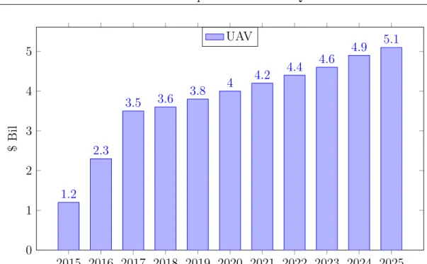
Based on this data the aerial drone market could cumulatively generate $ 91 billion over the next decade [7], with an estimate impact on the US market to be of about $ 5 billion in 2025 (Figure 2.4).
2014 2015 2016 2017 2018 0 1,000 2,000 3,000 4,000 5,000 13 47 44.3 53.7 66 330.2 409.8 408.6 429.7 381.8 3,775.9 4,819.4 4,467.6 4,217 4,419.3 $ Mil
Air Ground Maritime
Figure 2.3: DoD Unmanned Systems Funding in Millions of Dollars [81]. The funding is based on the 2014 Presidential Budget.
12 Chapter 2: UAV and Quadrotors: State of Art 2015 2016 2017 2018 2019 2020 2021 2022 2023 2024 2025 0 1 2 3 4 5 1.2 2.3 3.5 3.6 3.8 4 4.2 4.4 4.6 4.9 5.1 $ Bil UAV
Figure 2.4: Direct Economic Impact from the UAV Industry on the US Market. Source: Association For Unmanned Vehicle Systems International, 2013.
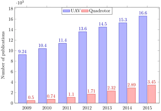
Further, based on the United States Department of Defense (DoD) report Un-manned Systems Integrated Roadmap [81], for the years 2013 ÷ 2038 the funding for unmanned systems (shown in Figure 2.3) will maintain a steady pace of investments, with an average of about $5 billion a year, with almost 90% of the funding reserved for unmanned aerial vehicles, whilst about 9 ÷ 10% is reserved to ground drones and what’s left to maritime drones. It is interesting to notice how little is the funding for maritime drones, symptom of an unripe technol-ogy, which is yet to come. This is due to the advantage of aerial vehicles: they are easier to build, control, and can be used almost anywhere in many applications. The United States is also the primary country for investments in the Research and Development sector (see Figure 2.5), with the goal to maintain incumbents in the country and keep the technological supremacy in the drone market. It is worth to point out that although Italy it is not amongst the top three countries in R&D, it has an average funding which is almost the same across the top European countries. It is also interesting to notice how many publications there are per year, in order to quantify on a first approximation the research done on the topic. For this reason Google Scholar was used as tool to quantify the amount of publications on the topics UAV and quadrotor: results are show in Figure 2.6 and they clearly present a positive trend, with more of 70% of publications focused on the control of UAVs vehicle.
2.2. Impact of Drones on Society and Developments 13 United States 56% China 12% Israel 9% Russia 8% Pan-European 3% Britain 2% France 2% Italy 2% Others 6%
Figure 2.5: Unmanned Aerial Systems - Research and Development by country (%) 2011-2020 forecast. Source: IHS Industry Research and Analysis; Teal Group
2009 2010 2011 2012 2013 2014 2015 0 2 4 6 8 10 12 14 16 18 ·10 3 9.24 10.4 11.4 13.6 14.5 15.3 16.6 0.5 0.74 1.1 1.71 2.32 2.89 3.45 Num ber of publications UAV Quadrotor
Figure 2.6: Number of articles indexed per year by Google Scholar for the topics UAV and Quadrotor.
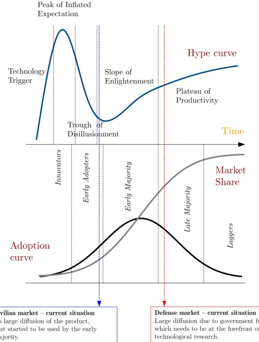
14 Chapter 2: UAV and Quadrotors: State of Art All of this information is sufficient to provide a first approximation of the diffusion of innovation curves, based on the theory of Rogers and Moore [69, 56], in which the diffusion of an innovation manifest itself in different ways and is highly subject to the type of adopters.
Rogers suggests a total of five categories of adopters in order to standardize the usage of adopter categories in diffusion research. The adoption of an innovation follows an S curve when plotted over a length of time. The categories of adopters are: innovators, early adopters, early majority, late majority and laggards. Given that the defense market is ahead of the civilian one, with lots of investment already planned, it is possible to say that drone technology for that market is already at a mature process, where the late majority is starting to adopt this technology. On the other hand the civilian market is behind, and the drone technology is starting only now to be diffused. This scheme is presented in Figure 2.7, along with the Gartner Technology Hype Curve, which is a curve describing the amount of hype
2.2. Impact of Drones on Society and Developments 15
Time
Hype curve
Adoption
curve
Peak of Inlated Expectation In n o va to rs E a rl y M a jo ri ty Technology Trigger Slope of Enlightenment Plateau of Productivity L a te M a jo ri ty L a gg er sDefense market – current situation
Large difusion due to government funds, which needs to be at the forefront of technological research.
Civilian market – current situation
No large difusion of the product, Just started to be used by the early majority.
Moore’s Segmentation and Hype Curve
Moore’s Segmentation and Hype Curve
Drone Market
Drone Market
Market
Share
E a rl y A d o p te rs Trough of Disillusionment16 Chapter 2: UAV and Quadrotors: State of Art
2.3
Adaptive Control of Quadrotors
Quadrotor vehicles are an interesting testbed for adaptive techniques. In fact, in designing a controller for these vehicles, there are multiple challenging questions to be addressed: actuator degradation, external disturbances, parameter uncer-tainties, time delays and actuator failures.
Adaptive control is therefore an attractive candidate to test its potential against the mentioned disturbances and uncertainties because of its ability to generate high performance tracking in presence of uncertainties. Its capability of learning whilst operating, and coping with uncertainties, made adaptive control the popular choice for fault-tolerant or reconfigurable flight.
Many approaches have been applied to quadrotors in a variety of problems: vision-based algorithms for indoor flight, dynamic programming for task assign-ment, autonomous tracking and regulation in indoor and outdoor settings and many others. Control approaches such as feedback linearization, machine learning and nonlinear controllers were used for agile maneuvers.
Unfortunately in the case of addditional uncertainties, due to failures, most approaches fail. Typical linear control law (PID control or linear-quadratic reg-ulator (LQR)) offer some measure of robustness, but it may not be sufficient for severe uncertainties. An example of controller, based on the MIT-rule, was designed to provide robustness in case of partial actuator failure [71]. However for the MIT rule there is no stability proof, and therefore the system cannot be guaranteed to be stable in general.
In the following sections some methods described in the literature to adaptively control quadrotors are presented. Main results and techniques are shown for standard MRAC and L1 schemes. Finally, other nonlinear adaptive techniques
used in literature are presented.
2.3.1
MRAC Schemes
MRAC is the most widely known adaptive control technique and there are many interesting results in control of quadrotor vehicles. A common characteristic of MRAC schemes is the use of a baseline controller, usually a PI controller designed by means of LQR.
In [18] the controller of a small quadrotor is augmented to include both a baseline fixed gain control and a model reference adaptive control. The whole system is equivalent to the baseline control in the nominal case, but in the case of a failure the adaptive control plays the role to maintain stability and regain the
2.3. Adaptive Control of Quadrotors 17 original performance. Although it is difficult to regain the original performance with a significant loss of thrust due to permanent damage in one of the four propellers, the Author has demonstrated that adaptive control allows for safe hover and return. Next a comparison with a CMRAC scheme was shown: the CMRAC controller was demonstrated to deliver smoother parameter estimates, allowing higher adaptive gains. It was shown that CMRAC was more effective than MRAC in learning the true value of uncertain parameters in the system, offering numerous benefits in terms of tracking performance.
An equivalent scheme is used in [21], where the Authors make use of a stan-dard baseline fixed gain control (which is a proportional plus integral controller) together with a Direct MRAC scheme. The Authors show how the adaptive controller is able to compensate uncertainties and provide better tracking perfor-mance than LQR in presence of mass uncertainty.
Also in [17] a baseline fixed gain control and direct model reference adaptive control are used to demonstrate the superior performance of MRAC compared to a non-adaptive scheme in case of actuator uncertainties, with a 45% loss of thrust failure. The adaptive controller exhibits significantly less deviation from level flight. The approach was validated using flight testing inside an indoor test facility, and the Projection Operator and the Dead Zone modification as robust tool modifications.
Of more interest are the adaptive schemes that make use of neural networks: the common denominator of those design is that the neural networks is added in order to approximate in a single term the uncertainty of the system, such as in the L1 piecewise-constant adaptive control where all uncertainties are lumped into
one parameter. Such approach is suitable for augmenting a baseline controller because does not require any modification of that baseline controller and the adaptive part can be added straightforwardly. Such approach is presented for example in [10, 12, 48, 37].
In [10] , [12] the neural network augments a nominal PID controller. The peculiar-ity of those schemes is the use of the concurrent learning modification (presented in Section 6.2.10), enabling a faster converge of the estimates to their true values. The control was designed so that an approximate inversion model is used in combination with a neural network that adaptively reduces the inversion error. Thanks to the concurrent learning modification the parameters of the neural networks converge more rapidly to their true values, leading to an improvement of the performances.
In [10] is shown the technique on two quadrotors of different sizes: the baseline controller is tuned for the bigger quadrotor and then tested on the other one, which
18 Chapter 2: UAV and Quadrotors: State of Art is half the size in comparison. Thanks to adaptive control nominal performances are restored, although the nominal controller was not optimised for the smaller quadrotor.
The very same idea is also used in [37] although without using the concurrent modification.
Instead in [48] the authors make use of a backstepping controller to control a quadrotor helicopter, successively augmented with a neural network that ac-counts for uncertainties.
Another design that makes use of adaptive backstepping is presented in [32], where only the mass of the vehicle is uncertain. In this work, however, the authors do not make use of a neural network but instead model the UAV with model parameters uncertainties and is mathematically more complex to design the adaptive controller since the backstepping design needs to be changed. For this reason neural networks are more beneficial, since when using them the nominal control does not have to be changed.
The method in [32], is further developed in [14], where also the vehicle’s mass, inertia matrix, and aerodynamic damping coefficients are assumed to be uncertain.
A different approach for approximating the uncertainty is given in [64]. This approach makes use of a fixed gain baseline controller augmented with the CMAC: a linear function approximation used to approximate the uncertainty. In practice a CMAC is a linear combination of N functions fi, i= 1, · · · , N, where each fi is equal to 1 inside of k square regions of input space, randomly scattered, and 0 everywhere else. Although the method shows good performances in presence of uncertainties, it is worth to point out that In comparison to neural networks, linear function approximation, such as CMAC, show worse performances since in general results indicate that nonlinear function approximators are more powerful for learning high-dimensional functions.
Finally, [1] proposes an interesting approach: the authors propose a LPV con-troller, synthesised by using the structured H∞ algorithm, based on the fact that
the controller parameters can vary in a certain domain given a set of uncertainties. Then, based on an indirect approach, by using a recursive least square algorithm the plant parameters are identified and used in the LPV controller. The method shows satisfactory performances and low jitter on the estimates, although no disturbances were introduced in the system.
2.3. Adaptive Control of Quadrotors 19
2.3.2
L
1Adaptive Control Schemes
Regarding L1 adaptive control there are some examples regarding UAVs, although
most of them make use of a nominal control of the type ub = −kx.
A different approach is shown in [49], where a nominal backstepping is designed to control the attitude of the quadrotor.
The baseline backstepping controller is successively augmented with a L1
piecewise-constant adaptive controller. Performances are visibly improved with adaptation, since fast adaptation is now possible due to the low-pass filter introduced in the L1
methodology. Further, also a scheme that makes use of quaternions is presented that avoids all singularities associated to Euler Angles.
In [54] the authors demonstrate an L1 adaptive output feedback control
de-sign, tuned by minimizing a cost function based on the characteristics of the reference model and the low-pass filter C(s). Flight test results shows that the augmented L1 adaptive system exhibits definite performance and robustness
im-provements. Also, adaptive augmentation is shown to help enable aggressive flight for a fixed-wing aerobatic aircraft.
L1 adaptive control in [3] is used to control a Miniature Air Vehicle: in fact
one of the challenges is that the manufacturing process for airframes is not consis-tent enough to ensure uniform aerodynamic properties. Hence adaptive control was used to account for those uncertainties and the effectiveness of the system was demonstrated through simulation results. The L1 adaptive algorithm results
in performance that exceeds the baseline PID controllers and exhibits robustness to a variable sample rate for the processor, as well as the time delays introduced by state estimation. The algorithm also appears to be robust with respect to state estimation noise.
Small unmanned air vehicles (UAVs) which makes use of L1 adaptive control [79]
have also been used to collect samples of pollen,and other biological particles, up to fifty meters altitude. In this work the L1 adaptive controller makes use of a neural
network to approximate the uncertainty, with guaranteed robustness and transient performance. Simulations illustrate the control designer’s ability to choose large adaptation gains for fast convergence without compromising robustness and also the fact that there is no need to re-tune the adaptive gains for different reference signals [79].
Part II
Adaptive Control: State-of-Art
“If you know the enemy and know yourself, you need not fear the result of a hundred battles. If you know yourself but not the enemy, for every victory gained you will also suffer a defeat. If you know neither the enemy nor yourself, you will succumb in every battle."
Chapter 3
Introduction to Adaptive Control
The words adaptive systems and adaptive control have been used as early as 1950, where the word to adapt generically means to change something to suit different conditions or uses.
Adaptive control was developed mainly in the aerospace field, where there was the need of autopilots for high-performance aircraft.
However, non-linearities, time-varying parameters and the fact that aircraft have to make more critical manoeuvres, represented problems which were difficult to tackle with the classical control theory. So far, the most common solution consists in linearising the aircraft model for a given flight condition, and design a controller for that situation, which can be tuned by means of the H∞ technique. Another
solution is the use of Linear parameter-varying control (LPV control), which provides a systematic design procedure for gain-scheduled regulators in order to control dynamical systems with varying parameters.
Unfortunately, the amount of work behind this process, and the fact that there is the possibility to encounter unpredicted flight conditions, led to the idea of designing an intelligent controller, able to adapt the controller parameters by processing the output of the sensors. This method led to the control structure on which adaptive control is based: a feedback loop where a block set is dedicated to dynamically adjust the control signals.
24 Chapter 3: Introduction to Adaptive Control
3.1
Short history of Adaptive Control
Adaptive Control has been a research topic of great interest since the early 50s: during that period there was a great interest in designing autopilots operating at a wide range of altitudes and speeds [25]. Self-tuning controllers, proposed by Kalman in 1958, and several schemes making use of the sensitivity rule or the MIT rules, were proposed for self-adjustment of the controller parameters. This was the consequence to the fact that linear control methods often are unable to provide proper stability margins and tracking performances in presence of highly non-linear characteristics. This led to high-gain feedback controllers to dominate nonlinearities and extensive use of gain-scheduling controllers.
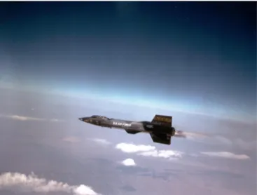
Figure 3.1: North American Aviation X-15A-3 56-6672 over Delamar Lake, Nevada (U.S. Air Force).
On the other hand adaptive control seemed to be a solu-tion to this problem, provid-ing consistent performances in presence of modeling uncertain-ties and unknown unknowns: is a nonlinear Solution to a non-linear Problem.
Adaptive control gave birth to the North American X-15 [16]: a hypersonic rocket-powered aircraft operated by the United States Air Force and NASA as part of the X-plane series of experimental air-crafts.
The X-15 airplane was one of the earliest featuring adaptive
control, making its first flight in 1959, recording nearly 200 successful flights from 1959 - 1968. In fact adaptive control seemed necessary to control hypersonic vehicles because of the changes in the aircraft dynamics as maneuver takes them over large flight envelopes.
In 1960s the X-15 set speed and altitude records, reaching the outer space, although the official world record for the highest speed ever recorded by a manned aircraft was set in October 1967, by William J. "Pete" Knight, who flew the X-15 at 7274km
h (Mach 6.72), and has remained unchallenged as of 2016.
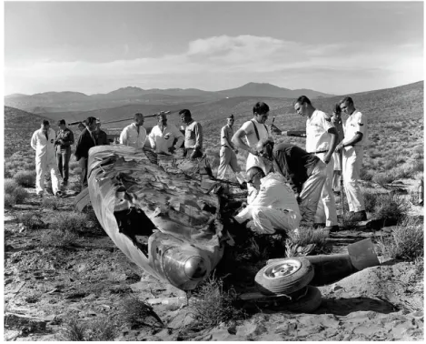
The program is largely considered a success, the one exception being the fatal accident that occured on November 15 in 1967 [16]. That event, in a sense, caused
3.1. Short history of Adaptive Control 25 the end of the program. During that flight the aircraft, after reaching its peak altitude, began a sharp descent entering a Mach 5 spin. The pilot was able to recover from the spin, but the adaptive controller was unable to reduce the pitch angle and consequently the aircraft continued to dive [16]. At about 20 km above the sea level the increasing pressure broke the aircraft apart. The lesson learned was that adaptive control is limited to slowly-varying uncertainties. In fact fast adaptation leads to high-frequency oscillations in control signal, which reduces the tolerance to time-delay in input/output channels.
Figure 3.2: Crushed forward fuselage of North American Aviation X-15A-3 56-6672 (NASA).
Years 1970-1990 have witnessed the development of formal methodologies for adaptive control systems, focusing on systems with parametric uncertainties, learnt the sobering lesson of tradeoffs between stability and performance and successively the birth of the Robust Adaptive Control paradigm.
In the early 1990s, the Air Force, Navy, and NASA cooperating with industry and academia have made significant process in developing reconfigurable adaptive flight control for aircraft and weapons [72].
Although many adaptive control methodologies were developed, almost all of them are restricted to slowly-time varying parameters in case of unmodelled dynamics that may cause instability of the system if excited.
This problem is what L1 adaptive control, born in 2006 [6], tries to solve. Up to
today there is still not a standard technique for adaptive control, although the L1
26 Chapter 3: Introduction to Adaptive Control
3.2
Adaptive Schemes
In the current literature there are two main categories of adaptive controllers, which are both formed by an on-line parameter estimator, also called adaptive law, and a control law motivated from the known parameter case. Specifically, the adaptive law provides an estimate of the unknown parameters, and is therefore an essential component of adaptive schemes, and it is thoroughly discussed in the fore-coming chapters.
The two approaches are called Direct Adaptive Control and Indirect
Adap-tive Control.
In the first approach, Direct Adaptive Control, the plant model is parametrized in terms of the controller parameters that are estimated directly without interme-diate calculations involving the estimates. This approach is also called Implicit Adaptive Control, since we are not estimating the true plant parameters but the controller gains. In direct adaptive control, the plant model itself is parametrized in terms of the unknown controller parameter vector, for which the controller meets the performance requirements, to obtain the plant model with unknowns to behave exactly with the same input/output characteristics of the nominal plant. Furthermore, the properties of the nominal plant model are crucial in obtaining the parametrized plant model that is convenient for on-line estimation. As a result, direct adaptive control is restricted to a certain class of plant models. Instead, in the second approach, Indirect Adaptive Control, the plant param-eters are first estimated on-line, then based on the identified model the control law is updated. It is therefore clear that, with this approach, the control law designed at each time t has to satisfy the performance requirements for the identified model, which in general differs from the true model of the plant.
Hence, the principal problem in indirect approaches is to choose the class of control laws and the class of parameter estimator as well as the algebraic equations that relates the unknown parameters estimates to the control law parameters to meet the performance requirements for the plant model with unknowns.
3.3. Adaptive Laws 27
3.3
Adaptive Laws
The idea behind the concept of Adaptive Control is the combination of an on-line parameter estimator with a control law. The combination of those two, given the large number of available methods used for parameter estimation and control laws, can give rise to a wide class of different adaptive controllers.
In the literature, the on-line parameter estimator is also referred to as the adap-tive law. The design of such adapadap-tive law is non-trivial and crucial for stability properties of the system. In fact, as we will see, it introduces a non-linearity that makes the closed-loop system nonlinear and often time-varying. Therefore, the stability and robustness analysis of adaptive control schemes are more challenging. The main methods used to design adaptive laws are:
• Sensitivity methods: one of the oldest method. It is based on the concept that the estimated parameters are adjusted in a direction that minimizes a certain performance function.
• Gradient methods and Least-Squares methods: Similar to sensitivity methods, but are based on the estimation error, which is a measure of the discrepancy between the estimated and actual parameters.
• Lyapunov design: the main method used nowadays. It is based on the direct method of Lyapunov, therefore providing a stability proof. The resulting adaptive law is very similar to the one obtained using sensitivity methods. This method is also used to predict transient and steady-state performance.
For more details on identification and estimation [34, 47] can be used as a starting reference.
3.3.1
Sensitivity methods
This class of methods, as previously aforementioned, is used to design the adaptive law so that the estimated parameters are adjusted in a direction that minimizes a certain performance function. It became very popular in the 1960s [13], and it is still widely used and it is one of the main examples used for introduction to adaptive control. Unfortunately, though, most formulations cannot be generated on-line, and those which can, have weak or undefined stability properties.
An example of such method, which led to the development of the MRAC theory, is the following: let y ∈ R be the plant output, and ym ∈ R the output of a reference model, and define the error difference as e = y − ym.
28 Chapter 3: Introduction to Adaptive Control Suppose the real plant depends on an unknown parameter vector θ ∈ Rn, i.e. , y= y(θ), then also the error depends on the unknown parameter vector e = e(θ). The control objective is to drive the output of the real plant so that
lim
t→∞e= 0. (3.1)
If the reference model differs from the real plant only for the unknown parameter θ, then a way of reducing e is to adjust θ in a direction that minimizes a certain cost function of e. An example is the quadratic function:
J(θ) = 1 2e
2(θ). (3.2)
A simple method to minimize J(θ) is the gradient method dθ dt = −Γ∇J(θ) = −Γe∇e(θ), ∇ = h ∂ ∂θ1, · · · , ∂ ∂θn iT ,Γ ∈ Rn×n (3.3)
where Γ > 0 is a diagonal matrix and a free design parameter, referred to as the adaptive gain. Then we can see that J is minimized over time, in fact its time derivative is always negative:
˙
J = e ˙e = e(∇e)T ˙θ. (3.4)
Since ˙J = ˙JT:
˙
J = e ˙θT∇e = −e2(∇e)TΓ∇e (3.5) Given that ym does not depend on θ, we have that ∇e = ∇y. Therefore the implementation of the adaptive law to estimate θ requires an on-line estimation of the sensitivity function ∇y. But y depends on the unknown plant parameters, which are unavailable. In these cases approximate values are used.
A popular method is the so-called MIT rule: with this rule the unknown parame-ters are replaced by their on-line estimates. But, in this way, it is not possible to prove closed-loop stability and performance properties.
3.3.2
Gradient and Least-Squares methods
One of the main drawback of sensitivity methods is that we obtain adaptive laws that are not implementable. A way to avoid this problem is to make use of performance criterion based on the estimation error: a measure of the discrepancy between the real and the estimated parameters.