1 23
Social Indicators Research
An International and Interdisciplinary
Journal for Quality-of-Life Measurement
ISSN 0303-8300
Volume 148
Number 2
Soc Indic Res (2020) 148:379-394
DOI 10.1007/s11205-019-02208-7
Measuring the Spatial Dimension of
Regional Inequality: An Approach Based
on the Gini Correlation Measure
1 23
Commons Attribution license which allows
users to read, copy, distribute and make
derivative works, as long as the author of
the original work is cited. You may
self-archive this article on your own website, an
institutional repository or funder’s repository
and make it publicly available immediately.
ORIGINAL RESEARCH
Measuring the Spatial Dimension of Regional Inequality:
An Approach Based on the Gini Correlation Measure
Domenica Panzera1 · Paolo Postiglione1 Accepted: 9 October 2019 / Published online: 19 October 2019 © The Author(s) 2019
Abstract
Traditional inequality measures fail to capture the geographical distribution of income. The failure to consider such distribution implies that, holding income constant, different spatial patterns provide the same inequality measure. This property is referred to as anonymity and presents an interesting question about the relationship between inequality and space. Particularly, spatial dependence could play an important role in shaping the geographical distribution of income and could be usefully incorporated into inequality measures. Fol-lowing this idea, this paper introduces a new measure that facilitates the assessment of the relative contribution of spatial patterns to overall inequality. The proposed index is based on the Gini correlation measure and accounts for both inequality and spatial autocorrela-tion. Unlike most of the spatially based income inequality measures proposed in the litera-ture, our index introduces regional importance weighting in the analysis, thereby differen-tiating the regional contributions to overall inequality. Starting with the proposed measure, a spatial decomposition of the Gini index of inequality for weighted data is also derived. This decomposition permits the identification of the actual extent of regional disparities and the understanding of the interdependences among regional economies. The proposed measure is illustrated by an empirical analysis focused on Italian provinces.
Keywords Inequality measure · Spatial patterns · Spatial autocorrelation · Inequality decomposition
JEL Classification C1 · C18 · R1 · R12
1 Introduction
Income inequality is an important social issue and a major concern for governments. It has inspired a long tradition of theoretical and empirical research and policies to address pov-erty and disparities. At the European level, reducing disparities between countries, regions
Disclaimer This paper reflects only the authors’ view. The Commission is not responsible for any use
that may be made of the information it contains. * Domenica Panzera
and social groups has inspired the European Union (EU) Cohesion Policy, and measures against poverty and social exclusion are among the specific objectives of the EU and its Member States (Molle 2007).
A number of studies that are concerned with the extent of inequality, its mechanisms and consequences have been proposed in the literature. For a review of the measures and methods that are frequently employed in the analysis of income inequality and income dis-tribution, see among others, Heshmati (2006) and Cowell (2011). The study of income ine-quality implies considering the income distribution between individuals or between regions in a country. The measurement of regional inequality generally relies on differences in regional GDPs rather than on income differences between individual or households within a regional economy (Rey and Janikas 2005). When regional inequality is analysed, there are some additional issues that need to be considered because of the nature of georefer-enced data and the possible spatial association relationships.
The literature on regional inequality has been mainly based on traditional inequal-ity measures and focused on their geographical decomposition (see among others, Max-well and Peter 1988; Tsui 1993; Fan and Casetti 1994; Kanbur and Zhang 1999; Nissan and Carter 1999; Azzoni 2001; Akita 2003; Beenstock and Felsenstein 2007). Studies on regional inequality based on composite indices resulting from the combination of multiple socio-economic indicators are also reported in the literature (Majumder et al. 1995; Quad-rado et al. 2001; Parente 2019). Some contributions in the recent literature highlighted some specific limitations of the studies on regional inequality (Rey and Janikas 2005; Portnov and Felsenstein 2010). An important issue that has been poorly explored in the literature con-cerns the relationship between spatial dependence and global inequality (Rey and Janikas
2005). Spatial dependence refers to the similarity between observations that are collected at near geographical locations. Spatial dependence could play an important role in shaping the geographical distribution of regional GDP since it implies that similar values tend to cluster together in space. However, the geographical distribution of GDP is mainly neglected in the measurement of inequality. In fact, traditional inequality measures, such as the Gini index or generalized entropy measures, are insensitive to the geographical arrangements of GDP. This implies that, holding GDP constant, different spatial patterns can provide the same inequality measure. This property of inequality measures is known as anonymity (Bicken-bach and Bode 2008). However, the joint consideration of measures of inequality and spatial dependence is desirable since it may reveal deeper insights about the distribution of regional GDP than would be possible using either measures alone (Rey and Janikas 2005).
The insensitivity of inequality measures to different spatial configurations has been addressed in a few recent contributions. Focusing on the relationship between measures of inequality and spatial dependence, Arbia (2001) suggested a number of approaches to combine them and developed some joint indexes. Arbia and Piras (2009) proposed a meas-ure based on the linear correlation coefficient that accounts for both spatial autocorrelation and variability. An alternative approach towards considering the joint effect of inequality and spatial autocorrelation, which relies on a decomposition of the Gini index, has been proposed by Rey and Smith (2013). Lastly, a decomposition of the Theil index T , which is aimed at capturing the neighbourhood effect on global inequality, has been proposed by Márquez et al. (2019).
Following this line of research, the present paper introduces a new measure that permits the quantification of the relative contribution of spatial patterns to overall inequality. Our measure relies on the Gini correlation measure that was introduced by Schechtman and Yitzhaki (1987), and assesses the association between the regional GDPs and the average GDP in neighbouring regions. As such, our measure offers a new interpretation of the Gini
correlation that traditionally has been used in the decomposition of the Gini index based on the income source (Lerman and Yitzhaki 1985; Ogwang 2016), in portfolio analysis in finance (Schechtman and Yitzhaki 1987), and in other fields such as biological science (Ma and Wang 2012).
In our proposal, the Gini correlation measure is used to identify the extent to which spatial dependence affects the regional inequality. As a further result, the proposed meas-ure introduces regional importance weighting in the analysis. This aspect has been mainly neglected from the studies on spatially based income inequality measures. Since we are dealing with regional data, GDP per capita is assumed to be the regional average income. To consider how many individuals this average represents, we consider GDP data that are weighted by population shares, and develop a measure that relies on the Gini index for weighted data as a measure of inequality (Mookherjee and Shorrocks 1982). A decomposi-tion of the Gini coefficient for weighted data into its spatial and non-spatial components is also derived.
The proposed measure is applied in an empirical analysis of regional inequality in Ital-ian provinces. Italy is characterized by a marked North–South dualism that is associated with relevant regional disparities. Accounting for spatial dependence in the analysis of such economic structures could improve the information that is derived from traditional inequality measures.
The remainder of this paper is organized as follows. Section 2 discusses the problem of the insensitivity of inequality measures to different spatial configurations of GDP. Sec-tion 3 introduces the proposed measure, gives some background information and presents its interpretation. In Sect. 4, the empirical analysis focused on regional inequality in Italian provinces is presented. Concluding remarks are given in Sect. 5.
2 Income Inequality and the Role of Space
The anonymity condition implies that traditional inequality measures are permutationally invariant, which means that very different spatial patterns can give rise to the same ine-quality measure.
With respect to the regional data, we consider the Gini index for weighted data G∗,1 where the GDP per capita for each region is weighted by the population share in the region with respect to the overall (i.e., national) population (Mookherjee and Shorrocks 1982; Yitzhaki and Schechtman 2013).
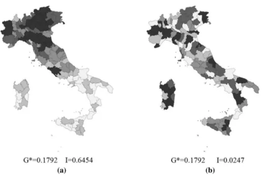
Figure 1(a) shows the geographical distribution of regional GDP per capita for the 110 Italian provinces in 2011, and (b) shows the geographical distribution that is obtained by randomly assigning the GDP per capita values to Italian provinces. The darker colours are used to indicate the provinces with higher GDP per capita, and the light colours refer to those with lower GDP per capita. The geographical distributions in Fig. 1 correspond to two different spatial patterns: the more agglomerated distribution is in (a) and the more dispersed distribution is in (b).
In addition, they are characterized by different degrees of spatial autocorrelation, as measured by Moran’s I2 (Moran 1950), while exhibiting the same level of inequality, as
measured by the Gini index.
This evidence brings up the importance of defining a measure that accounts for these differences and focuses on both inequality and spatial autocorrelation. Neglecting the spa-tial features of data in the measurement of inequality might mask important information about the actual disparities that are experienced by regional units. Thus, it becomes desir-able to define a measure that is desir-able to capture both the non-spatial variability, which is invariant to permutations, and the role of geographical location in economic inequality.
The particular geographical location of data is determined by the presence of positive or negative spatial associations, which makes consideration of the spatial dependence effect in the measurement of inequality relevant.
The importance of incorporating spatial dependence into inequality measures has been highlighted in some recent contributions. Focusing on the spatial concentration, Arbia (2001) emphasized the importance of developing indices that combine spatial autocorrela-tion and measures of variability, and suggested a number of different approaches. By mak-ing use of a series of empirical examples, the author showed that the spatial concentration consists of two different features as the a-spatial variability, which is invariant to permu-tations, and the polarization that refers to the geographical location of observations. To summarize these different aspects of spatial concentration, the author suggested combining
Fig. 1 Gini index G∗ and Moran’s I computed for GDP per capita—Italian provinces (2011) a Real spatial
distribution of regional GDP per capita, and b spatial distribution obtained by a random permutation of regional GDP per capita
2 Moran’s I computed for GDP per capita, y
i can be expressed as follows: I =∑ n
i ∑ jwij ∑ i ∑ jwij(yi−𝜇y)(yj−𝜇y) ∑ i(yi−𝜇y) 2 ,
the measures of the a-spatial concentration, such as the Gini index, or other measures of variability, with measures of spatial autocorrelation (like Moran’s I ) or measures of local association (like the Getis-Ord statistic) that measure polarization. The author gave some suggestions about the combination of these measures.
Arbia and Piras (2009) introduced a new class of measures that incorporates the ideas of both a-spatial concentration and spatial agglomeration. This class of measures is defined as the linear correlation coefficient between a random variable X that corresponds to n spa-tial units, and a random variable X∗ that corresponds to the permutation of the n values of X , which maximizes a measure of positive spatial association. Formally, we have the following:
where 𝜇 denotes the mean of Xi . This class of measures accounts for both the a-spatial
concentration (the variance in the denominator) and spatial correlation (the numerator). The authors discussed the properties of this measure and approximate sampling theory. They also identified some possible extensions of the proposed statistic, such as its use for the comparison of the concentration of the same variable measured over two different time periods or in two different countries, and its extension to other measures of inequality (see Arbia and Piras 2009).
Rey and Smith (2013) considered the Gini index G in its relative mean difference form, and rewrote the sum of all pairwise differences as the sum of absolute differences between pairs of neighbouring observations and absolute differences between pairs of non-neigh-bouring observations. Formally, we have the following:
where wij denotes the generic element of a binary spatial weight matrix expressing the
proximity relationship between locations i and j.
This decomposition facilitates the identification of a neighbouring component, NG , (i.e., the first term on the right side) and a non-neighbouring component, NNG , (i.e., the second term on the right side) of the Gini index G , and reveals that this index nests a meas-ure of spatial autocorrelation. In fact, when the amount of positive spatial autocorrelation strengthens, the second term should increase relative to the first since the value similarity in space would be greater. The result is the opposite in the presence of negative spatial autocorrelation (Rey and Smith 2013).
The contribution of Márquez et al. (2019) is focused on the Theil index T . Aiming at deter-mining the explicit contribution of spatial regional patterns to inequality, the authors iden-tified a neighbourhood Theil index that provides a measure of inequality that only consid-ers the information from the neighbouring regions. The identification of the neighbourhood Theil index allows one to separate the a-spatial and the spatial components of inequality. In fact, by subtracting the neighbourhood Theil from the conventional Theil, a Specific Theil index that accounts for non-spatial inequality is defined. The neighbourhood Theil index com-pletely depends on the concept of the neighbourhood and its quantification. Furthermore, it requires that the underlying spatial process be isotropic and significant; i.e., it is different from one that is derived by a completely random spatial process. Both these conditions make the (1) 𝜆= ∑n i=1�Xi− 𝜇��Xi∗− 𝜇 � ∑n i=1�Xi− 𝜇 �2 (2) G= ∑n i=1 ∑n j=1wij�� � xi− xj� � � 2n2𝜇 + ∑n i=1 ∑n j=1(1 − wij)�� � xi− xj� � � 2n2𝜇
replacement of the GDP in a region by the average GDP in neighbouring regions possible (see Márquez et al. 2019).
Following the idea of a complementarity between inequality and spatial autocorrelation, in this paper, we propose a measure that facilitates the assessment of the relative contribution of spatial patterns to a given pattern of income inequality. Our contribution is aimed at extending the previous works in this area. Our measure relies on the Gini index as a measure of global inequality. Using regional data, we focus on the Gini index that is computed using weighted data, and introduce a measure that can be interpreted as the ratio between a spatial Gini and this weighted Gini index. The introduced spatial Gini expresses the correlation between the regional GDP per capita and the same variable that is spatially lagged. As with the measure that was proposed by Arbia and Piras (2009), our index is thus defined as a ratio between a measure of spatial autocorrelation and a measure of variability. In the proposal by Arbia and Piras (2009), they state that assessing the extent of spatial autocorrelation requires the deter-mination of the spatial configuration that maximizes some spatial autocorrelation statistics. Our measure only requires the prior identification of the neighbouring regions for each spatial unit. As with the spatial decomposition that was proposed by Rey and Smith (2013), our con-tribution is focused on the Gini index of inequality. However, in our approach, a weighting scheme reflecting the relative importance of each region in the whole economy is considered, and the spatial relationships are defined using a single vector of weights.
In the contribution of Márquez et al. (2019), the spatial component is quantified by con-sidering only the information that is related to the neighbouring regions. In contrast, in our approach, the spatial Gini is based upon the correlation between the value that is observed for the reference unit and the values that are observed for the neighbouring regions.
3 The Proposed Measure: Background, Definition and Interpretation
The presence of positive or negative spatial associations impacts the geographical distribution of data. These associations should be considered in the analysis of regional inequality to prop-erly understand the differences in the GDP distributions. The importance of jointly consider-ing the spatial dependence and inequality requires the definition of a sconsider-ingle measure that could account for both of these aspects. The measure that is proposed in this paper is defined as a special case of the Gini correlation index that was introduced by Schechtman and Yitzhaki (1987).
The Gini correlation is a measure of association between two random variables, which is based on the covariance between one variable and its cumulative distribution function.
Let X and Y be two random variables with continuous distribution functions FX and FY ,
respectively, and a continuous bivariate distribution FX,Y . The Gini correlation is a not
sym-metric measure of association between X and Y . It can be specified in the following two forms, depending on which variable is given in its actual values and which is expressed through its cumulative distribution function:
or (3) 𝛤(x, y) = Cov(x, FY(y) ) Cov(x, FX(x) ) (4) 𝛤(y, x) = Cov(y, FX(x))
Cov(y, FY(y)
As Eqs. (3) and (4) show, the Gini correlation between two variables is expressed as the ratio of two covariances. The covariance in the numerator is computed between one vari-able and the cumulative distribution function of the other, and it corresponds to the Gini covariance between the variables. The covariance in the denominator is computed between the variable and its cumulative distribution function and represents a measure of variabil-ity. In fact, as showed by Schechtman and Yitzhaki (1987), the covariance in the denomi-nators of Eqs. (3) and (4) corresponds to one-fourth of the Gini’s mean difference, which is a measure of dispersion (see also, Stuart 1954).
The properties of the Gini correlation are a mixture of the properties of the Pear-son and Spearman correlations and have been detailed by Schechtman and Yitzhaki (1987), who defined a point estimator and derived its large sample properties (see also Schechtman and Yitzhaki 1999; Yitzhaki and Schechtman 2013). The main proper-ties of the index are listed below: (1) −1 ≤ 𝛤 (x, y) ≤ 1 for all (x, y) ; (2) if y is a mono-tonically increasing (decreasing) function of x , then both 𝛤 (x, y) and 𝛤 (y, x) will equal to + 1(− 1); (3) if x and y are statistically independent, then 𝛤 (x, y) = 𝛤 (y, x) = 0 ; (4)
𝛤(x, y) = −𝛤 (−x, y) = −𝛤 (x, −y) = −𝛤 (−x, −y) ; (5) 𝛤 (x, y) is invariant under a strictly
monotonic transformation of y ; and (6) 𝛤 (x, y) is invariant under scale and location changes in x . The proof of these properties is given in Schechtman and Yitzhaki (1987), which pro-posed some applications of the Gini correlation index in economics and finance.
The use of the Gini correlation for assessing the role that is played by a specified spatial configuration in the income distribution has been proposed by Dawkins (2007) in the field of income segregation, which refers to the uneven geographic distribution of households with different income levels within an area. This irregularity produces a pattern of inequal-ity. The measures of income segregation do not generally consider the spatial arrangement of neighbourhoods, thus giving rise to the checkerboard problem3 (see White 1983; Morrill 1991; Dawkins 2004, 2007).
To address this last issue, Dawkins (2007) introduced a new spatial ordering index Sr .
Two main spatial ordering schemes are emphasized by Dawkins (2007), including the nearest neighbour spatial ordering and the monocentric spatial ordering. The nearest neigh-bour spatial ordering assigns to each neighneigh-bourhood income the rank that is associated with the income per capita of the neighbourhood’s nearest neighbour. Conversely, in the monocentric spatial ordering, a new variable Z , expressing the distance from a given point within the region to the centroid of each neighbourhood, is defined. Then, the neighbour-hood incomes are ranked in ascending or descending order based on Z.
Based on these alternative spatial reranking schemes, the spatial ordering index Sr
is expressed as the ratio between a spatial reranked Gini index, Gr , and a Gini index of
between-neighbourhood income segregation, GB (see Dawkins 2007), as follows:
with Gr= (2∕Y)Cov(yj, ̄Rj(n) )
and GB= (2∕Y)Cov(yj, ̄Rj
)
, where Y is the aggregate house-hold income that is earned by the residents of the region, yj is the aggregate household
(5) Sr= Gr GB = Cov(yj, ̄Rj(n) ) Cov(yj, ̄Rj )
3 In the segregation literature, the checkerboard problem refers to the failure to distinguish between
differ-ent patterns of income segregation, ranging from clustered to spatially random, using common segregation measures.
income that is earned by the residents of the neighbourhood j , ̄Rj is the average rank of
the income per capita that is earned by neighbourhood j within the overall neighbourhood income per capita distribution, and ̄Rj(n) is the average spatial rank of the per capita income
that is earned by neighbourhood j . For further details, see Dawkins (2007).
Following Dawkins (2004, 2007), in this paper, we propose an index to evaluate the impact of the spatial dependence on inequality, which is defined starting with the Gini cor-relation measure that is defined in Eqs. (3) and (4).
Specifically, we introduce a measure that is defined as the Gini correlation between the variable Y and its spatial lag WY , where Y denotes the regional GDP per capita and W is a row-standardized spatial weight matrix that summarizes the proximity relationship between regional units. The spatially lagged variable expresses a weighted average of the values of Y that are observed for neighbouring regions.
Assuming, as a first simple working hypothesis, that all regional units are equally weighted (i.e., have the same population share), our measure, which is denoted as 𝛾 , can be specified as the ratio between the covariance of each observation of Y and the rank RWY of
the observations of WY and the covariance between Y and its own rank RY . It is as follows:
Denoted with n the number of observations, the expressions RY∕n and RWY∕n represent
the empirical estimates of the cumulative distribution functions of Y and WY , respectively (Yitzhaki and Lerman 1991), when the observations are equally weighted.
In Eq. (6), the numerator corresponds to the Gini covariance between Y and WY and provides a measure of spatial autocorrelation, while the denominator expresses the vari-ability in the regional GDP per capita.
Since the Gini index G can be expressed as twice the covariance between a variable and the rank of the variable divided by its mean (see Lerman and Yitzhaki 1984; Schecht-man and Yitzhaki 1987), the index 𝛾(y, Wy) can be rewritten as the ratio between a spatial reranked Gini Gs4 and the classic Gini index G:
where
and
where 𝜇y is the mean of the variable Y.
(6) 𝛾(y, Wy) = Cov(y, RWY∕n ) Cov(y, RY∕n ) (7) 𝛾(y, Wy) = Gs∕G (8) Gs= 2Cov(y, RWY∕n ) 𝜇y (9) G=2Cov(y, RY∕n ) 𝜇y
4 The term spatially reranked Gini, or simply spatial Gini, is borrowed from Dawkins (2004). In Dawkins
As previously mentioned, when dealing with regional data, the GDP per capita, which is assumed to be representative of the whole region, should be weighted by the region’s popu-lation to account for how many individuals this GDP per capita represents. This entails introducing a regional importance weighting in the analysis, which could be achieved by assigning the population shares 𝜋i= pi�∑ipi to each regional value yi where pi is the total
population of region i ; i = 1, 2, … , n ; and ∑i𝜋i= 1.
When using weighted data, Lerman and Yitzhaki (1989) suggested substituting the empirical cumulative distribution function in the covariance-based Gini formula with a quantity that reflects the idea of the midpoint of the cumulative distribution. Specifically, when each observation, yi , is associated with the weight, 𝜋i , the rank RY∕n in (9) can be
replaced by the following quantity (Lerman and Yitzhaki 1989):
where 𝜋0= 0.
Using the estimate of FY(y) from (10), we can calculate the weighted covariance
between y and FY(y) , and, hence, the Gini index for weighted data as follows:
where 𝜇∗ y = ∑ i 𝜋iyi , and ̄F∗=∑ i 𝜋iFY∗�yi�.
Following the same approach, a weighted version of the spatial Gini in (8) can be derived. The unweighted spatial Gini in (8) is based upon the covariance that is com-puted between the GDP per capita in each region and the rank that is associated with the weighted average GDP per capita in neighbouring regions divided by the number of obser-vations. To introduce the proposed weighted version of the spatial Gini, the GDP per capita values, yi , are reordered according to the non-decreasing order of the values assumed by
the weighted average GDP per capita in neighbouring regions, Wyi . Therefore, the rank
RWY∕n in (8) is replaced by the quantity F∗WY(Wyi
)
, which is defined similarly to Eq. (10). The weighted version of Gs is thus specified as follows:
where ̄F∗
W =
∑
i
𝜋iFWY∗ �Wyi�.
The weighted version of our index 𝛾(y, Wy) can be thus specified as follows:
Since, as discussed by Dawkins (2004), a spatial Gini index that is produced by a reranking will always be bounded above by the original Gini index and below by the nega-tive value of the Gini index, the index G∗
s is bounded below by −G
∗ and above by G∗ , and the following relation holds (see Dawkins 2004):
(10) F∗Y(yi) = i−1 ∑ j=0 𝜋j+ 𝜋i∕2 i = 1, 2, … , n (11) G∗=2Cov�y, F ∗ Y(y) � 𝜇∗y = 2∑n i=1𝜋i � yi− 𝜇∗ y � �F∗ Y�yi� − ̄F∗ � 𝜇y∗ (12) G∗S= 2Cov�y, F ∗ WY(Wy) � 𝜇y∗ = 2∑n i=1𝜋i � yi− 𝜇y∗ � �F∗ WY�Wyi� − ̄F∗W � 𝜇y∗ (13) 𝛾∗(y, Wy) = G∗S G∗ =
Cov(y, F∗WY(Wy))
Cov(y, F∗
Y(y)
Here G∗
ns , where 0 ≤ G
∗
ns≤2G
∗ , captures the component of the inequality that is not due to a specified pattern of spatial dependence. Equation (14) thus expresses the decomposition of the Gini index in its spatial and non-spatial components, and the relative contribution of the spatial component to the overall inequality is quantified by the measure 𝛾∗(y, Wy).
As previously mentioned, our measure, regardless of the weights used, ranges between −1 and 1 (Schechtman and Yitzhaki 1999; Ogwang 2016). When the ranking of WY is identical to the original ranking of Y , G∗
s= G
∗ , G∗
ns= 0 and 𝛾
∗(y, Wy) = 1, thus indicating that the overall inequality is completely explained by the given pattern of spatial depend-ence. As the ranking of the regional GDPs (i.e., Y ) becomes more dissimilar to the rank-ing of average GDPs in neighbour regions (i.e., WY ), the spatial component of inequal-ity decreases and it approaches its minimum value of −G∗ , when the average GDPs in neighbour regions are ranked as the opposite with respect to the original order of regional GDPs. In this case, the non-spatial component of inequality reaches its maximum value of 2G∗ and 𝛾∗(y, Wy) = −1 . When Y and WY are uncorrelated, we have that G∗
s = 0 , and,
thus, G∗= G∗
ns and 𝛾
∗(y, Wy) = 0 , thus indicating that the overall inequality is completely explained by its non-spatial component.
As with the measure that was introduced by Arbia and Piras (2009), our index is defined as a ratio between a measure of spatial autocorrelation and a measure of variability. Note that the weighted Gini covariance in the numerator of our measure expresses the correla-tion between the variable Y and its spatial lag WY . The Gini mean difference in the denom-inator of our measure shares many properties with the variance considered by Arbia and Piras (2009), but can be more informative with respect to the properties of distributions that depart from normality (see Yitzhaki 2003). Furthermore, in the measure that was pro-posed by Arbia and Piras (2009), assessing the extent of spatial autocorrelation requires determining the spatial configuration that maximizes some spatial autocorrelation statis-tics. In contrast, our measure only requires the prior identification of the neighbouring regions for each spatial unit. Furthermore, our measure is flexible enough to incorporate different proximity definitions.
As with the measure that was proposed by Rey and Smith (2013), our measure relies on the Gini index as measure of inequality. However, unlike Rey and Smith (2013), we consider the Gini index using weighted data. This introduces the differences in the contri-bution of regional economies to overall inequality into the analysis. This aspect has been mainly neglected in the previous literature on Gini based spatial inequality measures.
4 Empirical Illustration
The proposed measure is illustrated using empirical analysis that is focused on the income inequality in Italian provinces, that correspond to the NUTS 3 level of the official EU clas-sification. We consider regional GDP per capita data over the period of 2000–2015. The source of the data is the EUROSTAT dataset.
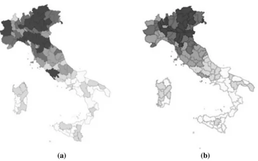
To illustrate the characteristics of our index, we first need to consider a spatial reranking of the geographical distribution of GDP per capita. To this end, Fig. 2 shows a comparison between the geographical distribution of regional GDP per capita in Italian provinces for 2011 (a) and the geographical distribution that is obtained by assigning the average GDP per capita of neighbouring provinces to each province (b). The spatial weight matrix W that (14)
is used in the definition of the proximity relationship is based on the k nearest neighbours’ criterion, where k = 5.
The weighted version of the measure that is proposed in Sect. 3 is computed by compar-ing the original order of regional GDPs in (a) with the rerankcompar-ing of the regional units based on (b). The weights that are assigned to y and Wy are assigned based on the share of the population in each region 𝜋i (see Sect. 3). The values of 𝛾∗(y, Wy) are reported in Table 1,
along with the values of the overall weighted Gini index G∗ and its spatial and non-spatial components. The results in Table 1 are also calculated using the diverse specifications of the matrix W that are based on different numbers of neighbours.
As Table 1 indicates, the results are stable for the different numbers of neighbours that are used in the definition of W . For any specification of the spatial weight matrix, we have positive values of the spatial Gini G∗
s . A positive value of G
∗
s reveals a positive association
between Y and WY . This result indicates the presence of positive spatial autocorrelation. For any specifications of the spatial weight matrix, the spatial component of the Gini index
G∗ is slightly larger than the non-spatial component G∗
ns. This indicates that for Italian
prov-inces, the global inequality is explained by both of these components roughly to the same extent. This result is confirmed by the value of 𝛾∗(y, Wy).
Fig. 2 Comparison between a the real spatial distribution of regional GDP per capita and b the spatial reranking based on the weighted average of neighbouring GDPs—Italy NUTS 3, year 2011
Table 1 Decomposition of the Gini Index G∗ for different patterns of spatial dependence (regional GDPs
per capita, Italy NUTS 3, year 2011)
W = 5 nearest neighbours W = 7 nearest neighbours W = 10 nearest neighbours
G∗ = 0.1792 G∗ = 0.1792 G∗ = 0.1792 G∗s = 0.0944 G∗s = 0.1002 G∗s = 0.0935 G∗ ns = 0.0848 G ∗ ns = 0.0790 G ∗ ns = 0.0857
Moreover, these results reveal that a positive spatial autocorrelation leads to increasing inequality because it gives rise to clusters of similar incomes. This result is consistent with some key findings in the regional inequality literature that revealed the presence of a posi-tive relationship between the measures of inequality and the degree of spatial autocorrela-tion (Rey 2004; Rey and Janikas 2005).
The results that are displayed in Table 1 reveal that the percentage impact of the spatial component to overall inequality is always higher than 50%. Some differences emerge if we consider a longer time period.
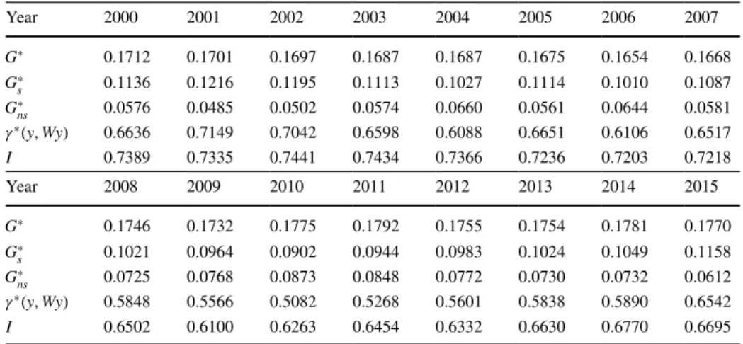
Table 2 shows the decomposition of the Gini Index G∗ into its spatial and non-spatial components for the period of 2000–2015. The values of Moran’s I , which are computed for the provincial GDP per capita, and the values of 𝛾∗(y, Wy) are also reported. The val-ues of the Gini index G∗ , and of its spatial and non spatial components, for the period of 2000–2015, are also depicted in Fig. 3.
As Table 2 indicates, for each year in the period under investigation, the spatial compo-nent of inequality is larger than the non-spatial compocompo-nent one (see also Fig. 3). The positive impact of the pattern of spatial autocorrelation to the overall inequality results in high values of 𝛾∗(y, Wy) , which are also depicted in Fig. 4. The presence of a positive spatial associa-tion is also confirmed by high values of the Moran’s I . The value of the spatial component of
Table 2 Spatial and non-spatial components of inequality for Italian provinces 2000–2015
Year 2000 2001 2002 2003 2004 2005 2006 2007 G∗ 0.1712 0.1701 0.1697 0.1687 0.1687 0.1675 0.1654 0.1668 G∗ s 0.1136 0.1216 0.1195 0.1113 0.1027 0.1114 0.1010 0.1087 G∗ ns 0.0576 0.0485 0.0502 0.0574 0.0660 0.0561 0.0644 0.0581 𝛾∗(y, Wy) 0.6636 0.7149 0.7042 0.6598 0.6088 0.6651 0.6106 0.6517 I 0.7389 0.7335 0.7441 0.7434 0.7366 0.7236 0.7203 0.7218 Year 2008 2009 2010 2011 2012 2013 2014 2015 G∗ 0.1746 0.1732 0.1775 0.1792 0.1755 0.1754 0.1781 0.1770 G∗ s 0.1021 0.0964 0.0902 0.0944 0.0983 0.1024 0.1049 0.1158 G∗ ns 0.0725 0.0768 0.0873 0.0848 0.0772 0.0730 0.0732 0.0612 𝛾∗(y, Wy) 0.5848 0.5566 0.5082 0.5268 0.5601 0.5838 0.5890 0.6542 I 0.6502 0.6100 0.6263 0.6454 0.6332 0.6630 0.6770 0.6695
Fig. 3 Gini index G∗ (points),
spatial component (grey dashed line), and non-spatial component (black dashed line)—Italy NUTS 3, 2000–2015
inequality and its impact on the overall inequality declines starting from 2008, as shown in Table 2 (see also Fig. 4). Our measure 𝛾∗(y, Wy) reaches its minimum value in 2010, and it increases starting from 2011. Note that the dynamics of our measure are consistent with the values of Moran’s I , which show a decline starting from 2008.
These results seem to have some important implications. First, the decrease of G∗
s ,
start-ing from 2008, reveals that the spatial spillovers are less evident durstart-ing the economic crisis. Second, the simultaneous increase of the non-spatial component of the Gini index reveals an effective increase in the inequality, which is masked by the values of G∗ that remain fairly sta-ble during all the periods under investigation (see Fig. 3).
Our results are in agreement with the empirical findings of the analysis that was given by Márquez et al. (2019). The authors, focusing on income inequality among European NUTS 3 regions, found a decrease of the relative importance of the neighbourhood component (as measured by the neighbourhood Theil index) and thus an increase in the specific component of inequality (measured by the specific Theil index) for the period of 2007–2014.
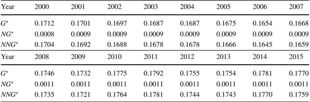
In Table 3, the spatial decomposition of the Gini index, which was proposed by Rey and Smith (2013), is presented. Specifically, we consider a weighted version of the decomposition given in Eq. (2), which is defined as follows:
with all variables being identical to those that are specified above. The first term on the right side represents the neighbouring component NG∗ , and the second one is the non-neighbouring component NNG∗ . The NNG∗ component can be interpreted as the spatial component of G∗ that varies in the same direction as the positive spatial autocorrelation (15) G∗= ∑n i=1 ∑n j=1wij𝜋i𝜋j�� � yi− yj� � � 2n2𝜇∗ y + ∑n i=1 ∑n j=1(1 − wij)𝜋i𝜋j�� � yi− yj� � � 2n2𝜇∗ y
Fig. 4 Relative contribution of spatial patterns to global inequal-ity—Italy NUTS 3, 2000–2015
Table 3 Neighbour and non-neighbour components of inequality for Italian provinces 2000–2015
Year 2000 2001 2002 2003 2004 2005 2006 2007 G∗ 0.1712 0.1701 0.1697 0.1687 0.1687 0.1675 0.1654 0.1668 NG∗ 0.0008 0.0009 0.0009 0.0009 0.0009 0.0009 0.0009 0.0009 NNG∗ 0.1704 0.1692 0.1688 0.1678 0.1678 0.1666 0.1645 0.1659 Year 2008 2009 2010 2011 2012 2013 2014 2015 G∗ 0.1746 0.1732 0.1775 0.1792 0.1755 0.1754 0.1781 0.1770 NG∗ 0.0011 0.0011 0.0011 0.0011 0.0011 0.0011 0.0011 0.0011 NNG∗ 0.1735 0.1721 0.1764 0.1781 0.1744 0.1743 0.1770 0.1759
(Rey and Smith 2013). Both these components, which are computed for Italian provinces over the period of 2000–2015, are reported in Table 3.
The results that are reported in Table 3 show a relevant positive contribution of the spa-tial component ( NNG∗) to overall inequality. The non-spatial component is fairly stable over the period under investigation.
Compared with these results, our measure seems to better emphasize the fluctuations of the spatial and non-spatial inequality over the period under investigation. Compared to the non-spatial component NG∗ , the non-spatial Gini, G∗
ns , permits one to better appreciate
the actual extent of the inequality and to isolate the role of spatial dependence in regional disparities. Compared to the spatial component NNG∗ of index G∗ defined in Eq. (15), the spatial Gini index G∗
s , that we introduced in Eq. (12), exhibits a trend that is more
coher-ent with the evolution, over the period 2000–2015, of the spatial dependence pattern, as measured by the Moran’s I . In fact, the Pearson’s correlation coefficient between G∗
s and
Moran’s I , over the 16 years, is 0.7424, while the Pearson’s correlation coefficient cal-culated between NNG∗ and I is − 0.7624. A strong positive relationship between our measure 𝛾∗(y, Wy) and the Moran’s I is also reported, with a Pearson’s correlation coef-ficient between these measures equal to 0.8381. In this sense, our measure, 𝛾∗(y, Wy) , that expresses the relative contribution of spatial dependence to a given pattern of regional ine-quality, assumes values that appear more coherent with the values of Moran’s I.
5 Conclusion
Dealing with regional inequality requires considering the role of spatial proximity in shap-ing the income distribution. However, traditional inequality measures disregard the geo-graphical location of data, and different spatial patterns may provide the same inequality measure.
To address this issue, this paper proposed an approach to assess the relative contribu-tion of a given spatial pattern to overall inequality. We introduced a measure that is defined using the regional GDP and the same variable that is spatially lagged, which is inspired by the Gini correlation (Schechtman and Yitzhaki 1987). Our measure, which is defined as 𝛾∗(y, Wy) , accounts for both the inequality and spatial autocorrelation and is the subject of an interesting interpretation as the ratio between the spatial reranked Gini index and the overall Gini index of inequality. Unlike most of the spatially based inequality indexes that have been proposed in the literature, our measure accounts for the different contributions of regions to the overall inequality. In fact, in the definition of our measure, we focus on a specification of the Gini index for weighted data. A decomposition of the Gini index in its spatial and non-spatial components is also derived.
The proposed approach is applied to analyse the regional economic inequality for Italian provinces over the period of 2000–2015. The empirical evidence showed a relevant contri-bution of the spatial dependence effect in shaping the inequality in Italian provinces. The spatial component contributes to the total inequality more than the non-spatial component for the period of 2000–2008, and it loses its relative importance during the economic crisis years. In fact, starting from 2008, we noted an increase in the relative importance of the non-spatial inequality. Our empirical findings are consistent with the empirical result of the study by Márquez et al. (2019).
Compared to the measure that was proposed by Rey and Smith (2013), our index appears to be more able to differentiate the contributions of the spatial and non-spatial
components of inequality, thereby highlighting a trend that is more consistent with that of Moran’s I.
This empirical evidence confirmed that the joint consideration of the spatial autocor-relation and income inequality produces important complementarities and offers insights that are not obtainable when these aspects are analysed alone. These results reveal that the proposed measure could be useful in assessing the actual extent of inequality, even in the presence of outstanding economic performances (Paredes et al. 2016). Furthermore, our measure is flexible enough to be applied at different geographical scales. The opportunity to identify the role of the spatial dependence relationship in driving income inequality at fine geographical scales is essential to providing useful information for location-based pol-icies that are aimed at reducing income inequality (Márquez et al. 2019).
Future research could further explore the properties of the proposed measure. Interest-ing areas for future research involve analysInterest-ing the impact of different neighbourhood defi-nitions and developing an inferential framework for the proposed measure.
Acknowledgements This study was financed by the project H2020 IMAJINE which has received funding from the European Union’s Horizon 2020 research and innovation programme under grant agreement No 726950.
Open Access This article is distributed under the terms of the Creative Commons Attribution 4.0 Interna-tional License (http://creat iveco mmons .org/licen ses/by/4.0/), which permits unrestricted use, distribution, and reproduction in any medium, provided you give appropriate credit to the original author(s) and the source, provide a link to the Creative Commons license, and indicate if changes were made.
References
Akita, T. (2003). Decomposing regional income inequality in China and Indonesia using two stage nested Theil decomposition method. The Annals of Regional Science, 37, 55–77.
Arbia, G. (2001). The role of spatial effects in the empirical analysis of regional concentration. Journal of
Geographical Systems, 3, 271–281.
Arbia, G., & Piras, G. (2009). A new class of spatial concentration measures. Computational Statistics &
Data Analysis, 53(12), 4471–4481.
Azzoni, C. R. (2001). Economic growth and income inequality in Brazil. The Annals of Regional Science,
31, 133–152.
Beenstock, M., & Felsenstein, D. (2007). Mobility and mean reversion in the dynamics of regional inequal-ity. International regional Science Review, 30(4), 335–361.
Bickenbach, F., & Bode, E. (2008). Disproportionality measures of concentration, specialization and locali-zation. International Regional Science Review, 31, 359–388.
Cowell, F. A. (2011). Measuring inequality (3rd ed.). Oxford: Oxford University Press.
Dawkins, C. J. (2004). Measuring the spatial pattern of residential segregation. Urban Studies, 41(4), 833–851.
Dawkins, C. J. (2007). Space and the measurement of income segregation. Journal of Regional Science,
47(2), 255–272.
Fan, C. C., & Casetti, E. (1994). The spatial and temporal dynamics of US regional income inequality, 1950–1989. The Annals of Regional Science, 28, 177–196.
Heshmati, A. (2006). The world distribution of income and income inequality: A review of the economics literature. Journal of World-Systems Research, 12(1), 61–107.
Kanbur, R., & Zhang, Y. (1999). Which regional inequality? The evolution of rural–urban and inland– coastal inequality in China, 1983-1995. Journal of Comparative Economics, 27, 686–701.
Lerman, R., & Yitzhaki, S. (1984). A note on the calculation and interpretation of the Gini index.
Econom-ics Letters, 15, 363–368.
Lerman, R., & Yitzhaki, S. (1985). Income inequality effects by income source: A new approach and appli-cations to the United States. Review of Economics and Statistics, 67(1), 151–156.
Lerman, R., & Yitzhaki, S. (1989). Improving the accuracy of estimates of the Gini coefficients. Journal of
Econometrics, 42, 43–47.
Ma, C., & Wang, X. (2012). Application of the Gini correlation coefficient to infer regulatory relationships in transcriptome analysis. Plant Physiology, 160, 192–203.
Majumder, A., Mazumdar, K., & Chakrabarti, S. (1995). Patterns of inter- and intra-regional inequality: A socio-economic approach. Social Indicators Research, 34, 325–338.
Márquez, M. A., Lasarte-Navamuel, E., & Lufin, M. (2019). The role of neighborhood in the analysis of spatial economic inequality. Social Indicators Research, 141(1), 245–273.
Maxwell, P., & Peter, M. (1988). Income inequality in small regions: a study of Australian statistical divi-sions. The Review of Regional Studies, 18, 19–27.
Molle, W. (2007). European Cohesion Policy. London: Routledge.
Mookherjee, D., & Shorrocks, A. (1982). A decomposition analysis of the trend in UK income inequality.
Economic Journal, 92(368), 886–902.
Moran, P. A. P. (1950). Notes on continuous stochastic phenomena. Biometrika, 37(1–2), 17–23. Morrill, R. L. (1991). On the measure of segregation. Geography Research Forum, 11, 25–36.
Nissan, E., & Carter, G. (1999). Spatial and temporal metropolitan and nonmetropolitan trends in income inequality. Growth and Change, 30, 407–415.
Ogwang, T. (2016). A new interpretation of the Gini correlation. Metron, 74(1), 11–20.
Paredes, D., Iturra, V., & Lufin, M. (2016). A spatial decomposition of income inequality in Chile. Regional
Studies, 50(5), 771–789.
Parente, F. (2019). A multidimensional analysis of the EU regional inequalities. Social Indicators Research,
143(3), 1017–1044.
Portnov, B. A., & Felsenstein, D. (2010). On the suitability of income inequality measures for regional analysis: Some evidence from simulation analysis and bootstrapping tests. Socio-Economic Planning
Science, 44, 212–219.
Quadrado, L., Heijman, W., & Folmer, H. (2001). Multidimensional analysis of regional inequality: The case of Hungary. Social Indicators Research, 56, 21–42.
Rey, S. J. (2004). Spatial analysis of regional income inequality. In M. Goodchild & D. Janelle (Eds.),
Spa-tially integrated social science: Examples in best practice (pp. 280–299). Oxford: Oxford University
Press.
Rey, S. J., & Janikas, M. V. (2005). Regional convergence, inequality, and space. Journal of Economic
Geography, 5, 155–176.
Rey, S. J., & Smith, R. J. (2013). A spatial decomposition of the Gini coefficient. Letters in Spatial and
Resource Sciences, 6, 55–70.
Schechtman, E., & Yitzhaki, S. (1987). A measure of association based on Gini’s mean difference.
Commu-nications in Statistics—Theory and Methods, 16, 207–231.
Schechtman, E., & Yitzhaki, S. (1999). On the proper bounds of the Gini Correlation. Economics Letters,
63, 133–138.
Stuart, A. (1954). The correlation between variate values and ranks in a sample from a continuous distribu-tion. British Journal of Statistical Psychology, 7, 37–44.
Tsui, K. Y. (1993). Decomposition of China’s regional inequalities. Journal of Comparative Economics, 17, 600–627.
White, M. J. (1983). The measurement of spatial segregation. American Journal of Sociology, 88, 1008–1018.
Yitzhaki, S. (2003). Gini’s Mean difference: A superior measure of variability for non-normal distributions.
METRON–International Journal of Statistics, 2, 285–316.
Yitzhaki, S., & Schechtman, E. (2013). The Gini methodology. A primer on a statistical methodology.
Springer Series in Statistics. New York: Springer.
Publisher’s Note Springer Nature remains neutral with regard to jurisdictional claims in published maps and institutional affiliations.