Comparing small area techniques for estimating poverty measures

QUADERNI DEL DIPARTIMENTO DI ECONOMIA POLITICA E STATISTICA

Federico Crescenzi Gianni Betti Francesca Gagliardi

Comparing small area techniques for estimating poverty measures

Comparing small area techniques for estimating poverty measures

Federico Crescenzi, Gianni Betti and Francesca Gagliardi Department of Economics and Statistics

University of Siena

Abstract

The Europe 2020 Strategy has formulated key policy objectives or so-called “headline targets” which the EU as a whole and Member States are individually committed to achieving by 2020. One of the five headline targets is directly related to key quality aspects of life, namely social inclusion; within these targets, the EU-SILC headline indicators at-risk-of-poverty or social exclusion and its components will be included in the budgeting of structural funds, one of the main instruments through which policy targets are attained. For this purpose, DG Regional Policy of the European Commission is aiming to use sub-national/regional level data (NUTS 2). Starting from this, the focus of the present paper is on the “regional dimension” of well-being. In fact, we compare two small area techniques, namely the cumulation and the spatial EBLUP (SEBLUP), on the basis of EU-SILC data from Austria and Spain.

Keywords: small area estimation; poverty; inequality; SILC JEL Classification: C21, I32, C23

Gianni Betti, Department of Economics and Statistics, University of Siena; email: gianni.betti@unisi.it; Federico Crescenzi, Department of Economics and Statistics, University of Siena; email:

federico.crescenzi@gmail.com; Francesca Gagliardi, Department of Economics and Statistics, University of Siena; email: gagliardi10@unisi.it

2

1. Introduction

In the last two decades there has been increased interest in comparative analysis of poverty and social exclusion in the European Union. The Statistical Office of the European Union (Eurostat) launched the European Community Household Panel study (ECHP, 1994-2001) and later the EU Statistics on Income and Living Conditions (EU-SILC, 2004-to date), in order to create a European standardised data base to generate comparative measures of poverty and social exclusion among the Member States. A comprehensive set of common indicators, termed the Laeken Indicators, has been adopted for countries of the European Union (Atkinson et al., 2002). These indicators are produced on a regular basis at national level, and are mainly based on the EU-SILC. EU-SILC surveys involve a rotational panel design conducted annually in each country. Microdata from the surveys are available to the research community in the form of a Users’ Data Base (UDB). The national sample designs and sizes have been determined primarily for the purpose of estimation and reporting of indicators at national level, with limited breakdown by major socio-demographic subgroups of the population.

The Europe 2020 Strategy (European Commission, 2010) has formulated key policy objectives or so-called “headline targets” which the EU as a whole and Member States individually are committed to achieving by 2020. One of the five headline targets is directly related to key quality aspects of life, namely social inclusion; within these targets, the EU-SILC headline indicators at-risk-of-poverty or social exclusion (AROPE, which is also known as Head Count Ratio (HCR) and FGT(0) in the family of Foster, Greer and Thorbecke, 1984) and its components will be included in the budgeting of structural funds, one of the main instruments through which policy targets are attained.

For this purpose, DG Regional Policy of the European Commission is aiming to use sub-national/ regional level data (NUTS 21_{, and exceptionally NUTS 1 for a couple of big} countries) for the social headline indicators, in order to complement GDP per capita, in defining regions that can apply for funding directed to the Convergence Objective. As a first step in this direction, for the funding period 2014-2020 these indicators will be used for benchmarking and assessing the efficiency of regional policies and programmes. Therefore, there is an urgent policy need for regional values of social policy indicators. The focus should be on accurately and correctly identifying regions with the highest proportion of people being poor or socially excluded, in order to target policy measures accordingly.

1 _{NUTS is an abbreviation for Nomenclature of Statistical Territorial Units. This is Eurostat’s hierarchical} classification of regions, from Member States (NUTS 0) down to smaller areas.

For these reasons, the focus of the present paper is on the “regional dimension” of well-being. While the above-mentioned EU-wide comparative data sets, namely the ECHP and the EU-SILC, can serve as unique sources for generating comparative indicators of well-being, or rather of lack of welfare manifest such as poverty and deprivation, these sources are designed primarily to serve at national level, and appropriate methodologies are required to extend their use to the level of sub-national regions: such methodologies are known as small area estimation (SAE) techniques.

There is a wide variety of techniques available (SAE) in the literature, and the field is rapidly expanding. The suitability and efficiency of a particular technique depends on the specific situation and on the nature of the statistical data available for the purpose. Standard reference on small area estimation methodology are Handerson (1950), Gosh and Rao (1994) and, above all, Rao (2003); Betti et al. (2012) focus on small area estimation methods for poverty and inequality measures.

One class of techniques aims at making the best use of available data from national sample surveys, such as by cumulating and consolidating the information to obtain more robust measures which permit greater spatial disaggregation; this class is described in Section 2, where the particular method of cumulating three-years of the EU-SILC survey is described and applied.

Another class of techniques is based on small area models; in the literature these are classified as: (i) area level random effect models (Fay and Herriot, 1979), which are used when auxiliary information is available only at area level (such as the prevailing unemployment rate); (ii) nested error unit level regression model, used if unit specific covariates (such as the individual’s or the household’s employment situation) are available at unit level (Battese et al., 1988).

In Section 3 one technique of class (i) is taken into account, namely the Empirical Best Linear Unbiased Predictor (EBLUP), and its developments in a spatial environment. One well known methodology of class (ii) is often undertaken by the World Bank, namely the Poverty Mapping (Elbers, Lanjouw and Lanjouw, 2003, ELL); however, it requires direct access to census data, which is not usually available for university researchers.

Finally, in Section 4 we compare the results obtained by the cumulation method and the spatial EBLUP (SEBLUP) method, based on Austria and Spain; some concluding remarks are also reported at the end of the paper.

Both methodologies applied in Sections 2 and 3 are based on the SILC, which is the major source of comparative statistics on income and living conditions in Europe. EU-SILC covers data and data sources of various types: cross-sectional and longitudinal; household-level and person-level; on income and social conditions; and from registers and interview surveys depending on the country. A standard integrated design has been adopted by nearly all EU countries. It involves a rotational panel in which a new sample

4

of households and persons is introduced each year to replace one quarter of the existing sample. Persons enumerated in each new sample are followed-up in the survey for four years. The design yields each year a cross-sectional sample, as well as longitudinal samples of various durations.

2. Cumulative measures of poverty

This section focuses on pooling of different sources pertaining to the same population or largely overlapping and similar populations. In particular, the interest is in pooling over survey waves in a national survey in order to increase the precision of regional estimates. Estimates from samples from the same population are most efficiently pooled with weights in proportion to their variances (meaning, with similar designs, in direct proportion to their sample sizes). Alternatively, the samples may be pooled at the micro level, with unit weights inversely proportional to their probabilities of appearing in any of the samples. This latter procedure may be more efficient (e.g., O’Muircheataigh and Pedlow, 2002), but may be impossible to apply as it requires information, for every unit in the pooled sample, on its probability of selection into each of the samples irrespective of whether or not the unit actually appears in the particular sample (Wells, 1998). Another serious difficulty in pooling samples is that, in the presence of complex sampling designs, the structure of the resulting pooled sample can become too complex or even unknown to permit proper variance estimation. In any case, different waves of a survey like EU-SILC do not correspond to exactly the same population. The problem is akin to that of combining samples selected from multiple frames, for which it has been noted that micro level pooling is generally not the most efficient method (Lohr and Rao, 1996). For the above reasons, pooling of wave-specific estimates rather than of micro data sets is generally the more appropriate approach to aggregation over time from surveys such as EU-SILC.

2.1 Gain in precision from cumulation over survey waves

Consider that for each wave of a survey like EU-SILC, a person’s poverty status (poor or non-poor) is determined from his/her income within the income distribution of that wave, independently for each EU-SILC year, and then the proportion of poor at each wave is computed. These proportions are then averaged over a number of consecutive waves.

The issue is to quantify the gain in sampling precision from such pooling, compared to results based on a single wave.

The quantification of efficiency gains from averaging across multiple years is not straightforward in surveys, such as EU-SILC, that are based on rotational panel, given that data from different waves of a rotational panel are highly correlated.

A large proportion of the individuals are common in the different cross-sections. However, a certain proportion of individuals are different from one wave to the other. The cross-sectional samples are thus not independent, resulting in correlation between measures from different waves.

Apart from correlations at the individual level, we have to deal also with additional correlation that arises because of the common structure (stratification and clustering) of the waves of a panel. Such correlation would exist in, for instance, samples coming from the same clusters even if there is no overlap in terms of individual households. In order to quantify the gain in precision from averaging over waves of a rotational panel, we provide the following simplified procedure that could be of help in better clarifying the point. It illustrates the statistical mechanism of how the gain is achieved. Indicating by pj and p'j the (1, 0) indicators of poverty of individual j over the two

adjacent waves, we have the following result for the population variances:









where ‘a’ is the persistent poverty rate over the two adjacent years.

Under the two waves model and in the extreme case of a completely full sample overlap and p p, the variance VA of the average over two waves of the concerned poverty measure can be estimated as:

(1 ) 2

A V

V    (1)

where ρ represents the correlation between the two waves that in our simplified case can be quantified by:

2 1 2 c a p V p p  _{  }   _     .

Alternatively, if the overlap between the two waves is only partial like in the EU-SILC survey, and cross-sectional variances are not necessarily equal, it is necessary to allow for variations in cross-sectional sample sizes and partial overlaps:

1 2 1 . . 1 . 2 2 A H V V n V n         _{  }    _     (2)

where V1 and V2 are the variances in each of the two waves, n is the sample overlap, nH

6

A replication method for variance estimation

The Jackknife Repeated Replication (JRR) is one of the classes of practical methods for variance estimation in complex samples based on measures of observed variability among replications of the full sample.

All replicated variance estimation procedures are based on comparisons among replications generated through repeated re-sampling of the same parent sample. Once the set of replications has been appropriately defined for any complex design, the same variance estimation algorithm can be applied to a statistic of any complexity.

The basic requirement is that the full sample is composed of a number of subsamples or replications, each with the same design and reflecting complexity of the full sample, enumerated using the same procedures. A replication differs from the full sample only in size. But its own size should be large enough for it to reflect the structure of the full sample, and for any estimate based on a single replication to be close to the corresponding estimate based on the full sample.

At the same time, the number of replications available should be large enough for the comparison among replications to give a stable estimate of the sampling variability in practice.

JRR provides a versatile and straightforward technique for variance estimation in situations like the ones we are concerned with.

Briefly, the standard JRR involves the following.

Let z be a full-sample estimate of any complexity. We use the subscript i to indicate a sample primary sampling unit (PSU) and h to indicate its stratum; ah≥2 is the number of

PSUs in stratum h. Let z(hi) be the estimate produced using the same procedure after

eliminating primary unit i in stratum h and increasing the weight of the remaining (ah-1)

units in the stratum by an appropriate factor gh (see below). Let z(h) be the simple

average of the z(hi) over the ah sample units in h. The variance of z is then estimated as:

 









  (3)

(1-fh) is the finite population correction and it is usually ~1 for samples in typical social

surveys.

While one may take factor gh as g_ha_h a_h1, it is more appropriate to use





h h h hi

g w w w , where w_h _iw_hi, with w_hi  _jw_hijas the sum of sample weights of ultimate units j in primary selection units i. This means that in each replication (hi), the weights for individual units are redefined and rescaled as follows: i) for unit j not in stratum h: w'_hij w_hij; ii) for unit j in stratum h but not in PSU i: w'_hij g_hw_hij; iii) unit j in

included sample cases unchanged across the replications created, so as to have the same total as the one for the full sample. With the sample weights scaled in such a way that their sum is equal (or proportional) to some external more reliable population total, population aggregates from the sample can be estimated more efficiently, often with the same precision as proportions or means (Verma and Betti, 2011).

2.2 Quantifying the gain in sampling precision using EU-SILC survey

The formulae presented in Section 2.1 have been applied to the EU-SILC cross-sectional datasets in order to obtain averaged measures over waves.

When complete information on sample structure is available and, more specifically, when identifiers are provided to link strata and PSUs throughout different EU-SILC cross-sectional datasets, it is possible to cumulate waves and quantify the gain in sampling precision achieved with this methodology.

When the above requirement is met, that is when full information on sample structure is available, the gain in sampling precision can be easily quantified by applying the standard JRR methodology presented above on the basis of the following considerations.

The total sample of interest is formed by the union of all the cross-sectional samples being compared or aggregated. Using the common structure of this total sample as a basis, a set of JRR replications is defined in the usual way.

Each replication is formed in such a way that when a unit is to be excluded in its construction, it is excluded simultaneously from every wave where the unit appears. For each replication, the required measure is constructed for each of the cross-sectional samples involved, and these measures are used to obtain the required averaged measure for the replication. Variance of the statistic of interest is then estimated from the replication estimates in the usual way.

Let us clarify this procedure, presenting an empirical example. Consider that we have the cross-sectional dataset of the EU-SILC survey for three consecutive years and want to estimate the average of a given poverty measure over the three years. We proceed as follows. We first construct a common structure of strata and PSUs from the union of the three cross-sectional datasets; that is, we keep the list of all the strata and PSUs of each of the three datasets and construct a new list that is the result of the union of the three samples. Then we will create the replications from this common structure. In the standard JRR methodology, replications are created by eliminating one PSU at a time, a replication being identified by the particular PSU (say k) eliminated in constructing it. In the combined dataset, the concerned PSU, if present, is eliminated from all the three cross-sectional datasets to obtain a ‘combined’ replication.

8

Next, we assign new weights to this common structure which are equal to the average of the weights of the three years:

(t)Common Average (1) (2) (3)

w =(w) =(w +w +w )/3 (4)

For each year (t) and for each replication (k), we can estimate (t) k

y where t=1, 2, 3 and from this, the required statistic

Average (t) t

k k

t

y =



that in our example on three waves is: Average (1) (2) (3)

k k k k

y =(y +y +y )/3. (6)

The variance estimate of this measure can be easily estimated applying the usual JRR for variance estimation procedure using the ‘combined’ replications as defined above, as if the statistic were a common cross sectional measure.

It is necessary to underline again that such procedures can be applied only if full information on the sample structure is available.

We have developed an alternative procedure for dealing with a situation in which full information on the sample structure is lacking (Verma et al., 2010).

2.3 Empirical results

We have applied the methodologies described above to calculate the average measures for three years (2009, 2010 and 2011) to EU-SILC data for Austria (AT) and Spain (ES). The empirical analysis has been performed only on these two countries for the following reasons. In the public version of the EU-SILC data, the so called UDB, the variables necessary for constructing the structure of the sample (namely, the PSUs ‘DB060’ and

k replication 1 2 3 waves A ll rep lica tio n s

the strata ‘DB050’) are not present and no link is possible across cross-sectional dataset either at micro (unit) level or at macro (structure) level. This problem is reflected also in Section 3.

Thanks to a project with the OECD for Spain we had access to all the necessary information on the sample structure and the linkage of the cross-sectional datasets. For Austria, all necessary information (linkage of the structure for the 3 cross sectional data sets) was not available to us, but, given that the Austria sample structure could be assimilated to a simple random sampling, we used for the computation the indirect procedure, mentioned above.

Results at the national level for Austria and Spain are shown in Table 1, and results at regional NUTS 2 level in Austria and Spain in Table 2 and 3.

Table 1 Average over three years, Austria and Spain.

(a) (b) (c) (d) AUSTRIA HCR 60% national p.l. 13.8 0.608 0.426 0.700 S80/S20 4.0 0.084 0.066 0.786 SPAIN HCR 60% national p.l. 22.0 _{0.478 0.311 0.650} S80/S20 6.5 0.154 0.110 0.718 (a) Estimate 2011 (b) s.e. 2011

(c) s.e. 3-years average

(d) ratio s.e. 3-years average over s.e. single year

The results at national level show a sensible reduction of the standard error (s.e.) using the three years average with the two measures concerned. The reduction of the standard errors that we get using the three years averages compared to the estimate for a single year (column (d)), ranges from 12% for S80/S20 index for Austria, up to 35% for HCR for Spain. In general the two methodologies (direct and indirect) for the estimation of standard errors of averaged measures over three years perform well and give similar results both at national and regional level, as we have already shown in our past work. The comparison of standard errors between one-year and three-year estimates is more complex at regional NUTS 2 level, given the instability of the one-year estimates because of small samples. This problem is particularly evident for regions with a small number of PSUs. The cumulated estimates in fact have been chosen to overcome to the high instability of the single year estimates.

10

Generally, also in this case we can appreciate a reduction of the standard error, both in mean and median, for the two measures. The reduction can be better appreciated considering the median, which is not affected by extreme values that are present in the results given the instability of the estimates for single years.

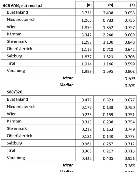
Table 2. Average over three years, Austria regional NUTS 2 level. HCR 60%, national p.l. (a) (b) (c) Burgenland _{3.721 2.438 0.655} Niederösterrich 1.065 0.783 0.735 Wien _{1.859 1.352 0.727} Kärnten _{3.347 2.240 0.669} Steiermark 1.297 1.100 0.848 Oberösterrich _{1.119 0.718 0.642} Salzburg 1.877 1.323 0.705 Tirol _{1.914 1.146 0.599} Voralberg _{1.989 1.595 0.802} Mean 0.709 Median _0.705 S80/S20 Burgenland _{0.477 0.323 0.677} Niederösterrich 0.177 0.138 0.780 Wien _{0.225 0.169 0.751} Kärnten 0.315 0.238 0.754 Steiermark _{0.218 0.163 0.749} Oberösterrich _{0.181 0.140 0.773} Salzburg 0.361 0.257 0.712 Tirol _{0.303 0.217 0.715} Voralberg _{0.425 0.405 0.951} Mean 0.763 Median _0.751 (a) s.e. 2011

(b) s.e. 3-years average

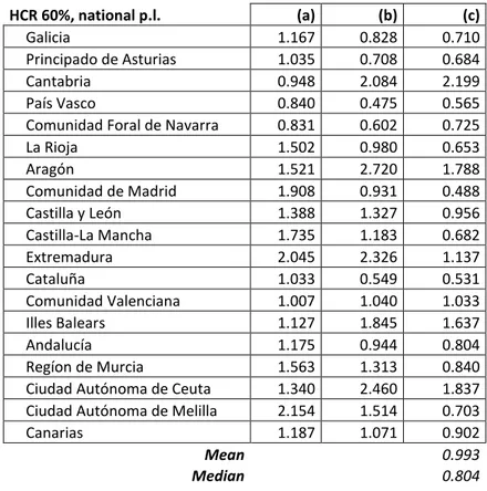
Table 3a. Average over three years, Spain regional NUTS 2 level, HCR. HCR 60%, national p.l. (a) (b) (c) Galicia 1.167 0.828 0.710 Principado de Asturias 1.035 0.708 0.684 Cantabria 0.948 2.084 2.199 País Vasco 0.840 0.475 0.565

Comunidad Foral de Navarra 0.831 0.602 0.725

La Rioja 1.502 0.980 0.653 Aragón 1.521 2.720 1.788 Comunidad de Madrid 1.908 0.931 0.488 Castilla y León 1.388 1.327 0.956 Castilla-La Mancha 1.735 1.183 0.682 Extremadura 2.045 2.326 1.137 Cataluña 1.033 0.549 0.531 Comunidad Valenciana 1.007 1.040 1.033 Illes Balears 1.127 1.845 1.637 Andalucía 1.175 0.944 0.804 Regíon de Murcia 1.563 1.313 0.840

Ciudad Autónoma de Ceuta 1.340 2.460 1.837 Ciudad Autónoma de Melilla 2.154 1.514 0.703

Canarias 1.187 1.071 0.902

Mean 0.993

Median 0.804

The results are very stable across regions in Austria. Furthermore, the results for mean and median measures are nearly the same, showing a reduction in variance of about 25-30% with pooling over 3 years.

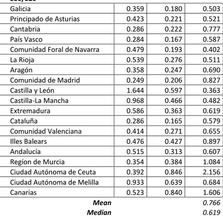
For Spain the largest reductions in this case are in S80/S20, where, in median, we have a decrease of 38%; for HCR the decrease in median is 20%.

12

Table 3b. Average over three years, Spain regional NUTS 2 level, S80/S20. S80/S20

Galicia 0.359 0.180 0.503

Principado de Asturias 0.423 0.221 0.521

Cantabria 0.286 0.222 0.777

País Vasco 0.284 0.167 0.587

Comunidad Foral de Navarra 0.479 0.193 0.402

La Rioja 0.539 0.276 0.511 Aragón 0.358 0.247 0.690 Comunidad de Madrid 0.249 0.206 0.827 Castilla y León 1.644 0.597 0.363 Castilla-La Mancha 0.968 0.466 0.482 Extremadura 0.586 0.363 0.619 Cataluña 0.286 0.165 0.579 Comunidad Valenciana 0.414 0.271 0.655 Illes Balears 0.476 0.427 0.897 Andalucía 0.515 0.313 0.607 Regíon de Murcia 0.354 0.384 1.084

Ciudad Autónoma de Ceuta 0.392 0.846 2.156 Ciudad Autónoma de Melilla 0.933 0.639 0.684

Canarias 0.523 0.840 1.606

Mean 0.766

Median 0.619

(a) s.e. 2011

(b) s.e. 3-years average

(c) ratio s.e. 3-years average over s.e. single year

3. Model based small area estimation

In this section we present the main features of some model-based techniques for small area estimation, namely, the EBLUP estimator based on the model by Fay and Herriot (1979) and the EBLUP estimator based on spatially correlated random effects (Pratesi and Salvati, 2007). The first is an essential tool in dealing with small area estimation when only aggregated auxiliary data at the area level are available, the latter allows for spatial dependence of area level random effects by assuming a Simultaneously Autoregressive Process (SAR). We have applied these estimators to a pair of poverty and inequality measures, namely Head Count Ratio and the S80/S20 index.

3.1 Empirical Best Linear Unbiased Predictor

We are interested in obtaining an estimate of a domain specific parameter 𝜃𝑖 (𝑖 = 1,2, … , 𝑚). In this work it can be either HCR or S80/S20. As true values 𝜃𝑖 are unknown it is assumed that a design-based unbiased estimator of the parameter is available such that 𝜃̂𝑖= 𝜃𝑖+ 𝑒𝑖, where 𝑒𝑖 (𝑖 = 1, 2, … , 𝑚) , are the sampling errors for each area, independent of each other and distributed with mean 0 and variance 𝜓𝑖. This is known as sampling model. It is assumed that the sampling variances 𝜓𝑖 are known, but in practice it is rarely the case, so they are replaced with estimates 𝜓̂𝑖 obtained by following a JRR procedure (Verma, 2004).

It is further assumed that true values 𝜃𝑖 are linearly related to a vector of 𝑝-area specific auxiliary variables 𝒙𝑖= (𝑥1𝑖, 𝑥2𝑖, … , 𝑥𝑝𝑖)𝑇:

𝜃𝑖= 𝒙𝑖′𝜷 + 𝑧𝑖𝑣𝑖

where 𝑣𝑖~(0, 𝜎𝑣2) are independent area-level random effects. Normality of random effects can be assumed to obtain Maximum Likelihood (ML) or Restricted Maximum Likelihood (REML) estimates 𝜎̂𝑣2 _{. This model is known as linking model.}

By combining the results above the Fay and Herriot (1979) model is obtained: 𝜃̂_𝑖 = 𝒙_𝑖′_{𝜷 + 𝑧}

𝑖𝑣𝑖 + 𝑒𝑖 (7)

where 𝑣𝑖 are independent of 𝑒𝑖. Under the model we have 𝐸[𝜃̂𝑖] = 𝒙𝑖′𝜷 and

𝑉[𝜃̂𝑖] = 𝜓𝑖+ 𝑧𝑖2𝜎𝑣2. The Best Linear Unbiased Predictor of 𝜃𝑖 can be easily obtained by applying the general results of linear mixed effects models and it is equal to:

𝜃̃_𝑖𝐻_(𝜎

𝑣2) = 𝛾𝑖𝜃̂𝑖 + (1 − 𝛾𝑖)𝒙𝑖′𝜷̃ (8)

where factor 𝛾𝑖= 𝑧𝑖2𝜎𝑣2/(𝜓𝑖+ 𝑧𝑖2𝜎𝑣2) is known as shrinkage factor and 𝜷̃ is the BLUE estimator of 𝜷. The expression above shows that the BLUP estimator is an average of the direct estimator 𝜃̂𝑖 and the synthetic estimator 𝒙𝑖′𝜷̃. It can be noted that the lower the sampling variance is the more the weight is attached to the direct estimator 𝜃̂𝑖 , in fact when 𝜓𝑖→ 0 then 𝛾𝑖→ 1 meaning that 𝜃̃𝑖𝐻→ 𝜃̂𝑖. We can say that the BLUP estimator is design consistent. In matrix notation the model can be expressed as:

𝜽

̂ = 𝑿𝜷 + 𝒁𝒗 + 𝒆 (9)

The BLUP estimator is unknown as it depends on random effects variance 𝜎𝑣2. By substituting it with a consistent estimator 𝜎̂𝑣2 _{we obtain a two stage estimator which can} be referred to as Empirical BLUP (EBLUP) and it is indicated as 𝜃̂𝑖𝐻_{= 𝜃̃𝑖}𝐻_(𝜎̂

𝑣2) = 𝛾̂𝑖𝜃̂𝑖+ (1 − 𝛾̂𝑖)𝒙𝑖′𝜷̂. Under the model (7) the MSE of the BLUP estimator is:

MSE[𝜃̃𝑖𝐻] = E[𝜃̃𝑖𝐻− 𝜃𝑖] = 𝑔1𝑖(𝜎𝑣2) + 𝑔2𝑖(𝜎𝑣2) Where: 𝑔1𝑖(𝜎𝑣2) = 𝜓𝑖[1 − 𝛾𝑖] 𝑔2𝑖= 𝛾𝑖2+ 𝒙𝑖′{∑(𝜎𝑣2+ 𝜓𝑖)−1 𝑚 𝑖=1 𝒙𝒊𝒙𝑖′} −1 𝒙𝑖

14

where 𝑔1𝑖(𝜎𝑣2_{) is due to the prediction of the random effect 𝑣𝑖 and is 𝑂(1) for large 𝑚, 𝑔2𝑖} is due to the estimation of 𝜷 and is 𝑂(𝑚−1_{). This means that a large reduction in MSE} over MSE(𝜃̂𝑖) = 𝜓𝑖 can be obtained when 1 − 𝛾𝑖 is large.

Under normality of random effects and errors, the MSE of the EBLUP is: 𝑀𝑆𝐸(𝜃̂𝑖𝐻_{) = 𝑀𝑆𝐸[𝜃̃𝑖}𝐻_{] + 𝐸[𝜃̂𝑖}𝐻_{− 𝜃̃𝑖}𝐻_{] = 𝑔1𝑖(𝜎}

𝑉2) + 𝑔2𝑖(𝜎𝑣2) + 𝑔3𝑖(𝜎𝑣2) + 𝑜(𝑚−1)

where 𝑔3𝑖(𝜎𝑣2) = 𝛾𝑖2(𝜎𝑣2+ 𝜓𝑖)−1 𝑉̅(𝜎̂𝑣2), and 𝑉̅ is the asymptotic variance of the estimator 𝜎̂𝑣2. The classic Fay and Herriot model (7) can be extended by considering that the vector 𝒗 follows a Simultaneously Autoregressive Process (SAR) with spatial autoregressive coefficient 𝜌 and proximity matrix 𝑾 (Cressie, 1993).

𝒗 = 𝜌𝑾𝒗 + 𝒖 → 𝒗 = (𝑰 − 𝜌𝑾)−1_{𝒖 (10)}

where 𝒖~𝑵(𝟎, 𝜎𝑢2_{𝑰) which implies that 𝒗 has mean vector 0 and variance-covariance} matrix

𝑮 = 𝜎𝑢2_{[(𝑰 − 𝜌𝑾)(𝑰 − 𝜌𝑾}𝑇_)]−1_.

Combining equations (9)-(10) the model with spatially correlated random effects is: 𝜽

̂ = 𝑿𝜷 + 𝒁(𝑰 − 𝝆𝑾)−𝟏_{𝒖 + 𝒆 (11)}

Under the model above the covariance matrix of the estimator 𝜽̂ is 𝑽 = 𝑹 + 𝒁𝑮𝒁𝑇_, where 𝑹 = 𝑑𝑖𝑎𝑔(𝜓𝑖) is the covariance matrix of the error term 𝒆.

Matrix 𝑾 describe the spatial contiguity among areas while 𝜌 ∈ [−1,1] describes the strength of spatial relationship among the random effects associated with neighbouring areas.

Under the model (11) the Spatial Best Linear Unbiased Predictor is: 𝜽 ̃_𝒊𝑺_(𝝈 𝒖 𝟐_{, 𝝆) = 𝒙} 𝒊𝜷̃ + 𝒃𝒊𝑻{𝝈𝒖𝟐[(𝑰 − 𝝆𝑾)(𝑰 − 𝝆𝑾𝑻)]−𝟏}𝒁𝑻{𝒅𝒊𝒂𝒈(𝝍𝒊) + 𝒁𝝈𝒖𝟐[(𝑰 − 𝝆𝑾)(𝑰 − 𝝆𝑾𝑻_)]−𝟏_𝒁𝑻_}−𝟏_{(𝜽̂ − 𝑿𝜷̃) (12)}

which is equal to the classic BLUP if 𝜌 = 0.

The estimator is unknown because it depends on the unknown parameters 𝜎𝑢2 and 𝜌. By substituting them with a consistent estimator (ML or REML) 𝜎̂𝑢2 _{and 𝜌̂ a two stage} estimator 𝜃̂𝑖𝑆_{= 𝜃̃𝑖}𝑆_(𝜎̂𝑢2_{, 𝜌̂) is obtained which can be referred to as a Spatial EBLUP (Pratesi} and Salvati, 2007).

The spatial weight matrix reflects the neighbouring structure of the small areas. In the next applications the structure has been specified by following an approach based on contiguity and on distance threshold (see Cliff and Ord, 1981, for further details). The former specifies the spatial dependence between two areas by assigning spatial weigh 𝑤𝑖𝑗= 1 if area 𝑖 and 𝑗 are adjacent and zero otherwise. The latter assigns spatial weight 𝑤𝑖𝑗 = 1 if the distance between the centroid of area 𝑖 and 𝑗 is less than a distance threshold 𝜏. Generally, the matrix 𝑾 is row-standardized, so it is row-stochastic and 𝜌

Under the model (12) the Mean Square Error of the Spatial BLUP estimator depending on two variance components (𝜌, 𝜎𝑣2) is given by:

MSE[𝜃̃_𝑖𝑆_{(𝜌, 𝜎}

𝑢2)] = 𝑔1𝑖(𝜌, 𝜎𝑢2) + 𝑔2𝑖(𝜌, 𝜎𝑢2)

where the first term is due to the estimation of random effects and it is of order 𝑂(1), while the second is due to the estimation of 𝜷 and it is of order 𝑂(𝑚−1).

For the Spatial EBLUP, given the normality of random effects, we have: MSE[𝜃̃_𝑖𝑆(𝜌̂, 𝜎𝑢2)] = MSE[𝜃̃𝑖𝑆(𝜌, 𝜎𝑢2)] + E[𝜃̃𝑖𝑆(𝜌̂, 𝜎̂𝑢2) − 𝜃̃𝑖𝑆(𝜌̂, 𝜎̂𝑢2)]

The last term is intractable and therefore it needs to be approximated. For full details on the MSE of the spatial EBLUP and its estimation procedure, see Pratesi and Salvati (2007).

3.2 Applications

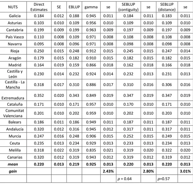
In this section we apply the above estimators to EU-SILC data available for Austria and Spain at NUTS 2 level. We have 16 NUTS 2 for Spain and 9 NUTS 2 for Austria at our disposal. Following Bivand, Rubio, and Pebesma (2008) there are basically three different types of spatial data: 1) Spatial Point Processes 2) Geostatistical data 3) Areal Data. In this paper we focus on areal data which means that when it is collected data regard a particular region, country, small area of any kind. The aim is to investigate how and to what extent data observed in one region is influenced by what has been observed in other regions. Tables 4 and 5 show direct, EBLUP and SEBLUP estimates. The gain in efficiency is quantified on the following lines: for each area we calculate the ratio between the estimate of the standard error obtained by the model-based estimator and the estimate of the standard error of the direct estimate. Then, these values are averaged to get the gain in efficiency.

Table 4 shows that the Spatial EBLUP based on a distance approach (𝜃̂_𝑖𝑆𝑑_{) leads to the} highest gain in efficiency. The gain is quite small, this is due to the fact that the direct estimates of HCR already have an appropriate level of accuracy. Proof of this can be had by observing the estimates of the shrinkage factors which are all close to 1. This means that, in traditional EBLUP case, the weight is attached mostly to the direct estimates rather than to regression estimate meaning that sampling variances 𝜓̂𝑖 are small with respect to the total model-variance.

Regarding the S80/S20 Index, the results in Table 5 show that the highest gain in efficiency is obtained with the traditional EBLUP. This is not surprising because the estimated spatial autocorrelation coefficient is lower than the one estimated in the HCR case. It is interesting to note that when the coefficient is almost zero, the estimates obtained with EBLUP and SEBLUP are nearly the same. In fact, when 𝜌 = 0 the EBLUP and SEBLUP estimators are equal (Bivand, Rubio and Pebesma, 2008).

16

Table 4. HCR Estimates. Spain 2011

NUTS Direct

Estimates SE EBLUP gamma se

SEBLUP (contiguity) se SEBLUP (distance) se Galicia 0.184 0.012 0.188 0.945 0.011 0.184 0.011 0.183 0.011 Asturias 0.103 0.010 0.109 0.956 0.010 0.109 0.010 0.109 0.010 Cantabria 0.199 0.009 0.199 0.963 0.009 0.197 0.009 0.197 0.009 País Vasco 0.110 0.008 0.109 0.971 0.008 0.108 0.008 0.108 0.008 Navarra 0.095 0.008 0.096 0.971 0.008 0.098 0.008 0.098 0.008 Rioja 0.250 0.015 0.248 0.912 0.015 0.245 0.015 0.247 0.014 Aragón 0.179 0.015 0.182 0.910 0.015 0.182 0.015 0.182 0.015 Madrid 0.164 0.019 0.159 0.866 0.018 0.162 0.018 0.166 0.018 Castilla y León 0.230 0.014 0.232 0.924 0.014 0.232 0.013 0.231 0.013 Castilla - La Mancha 0.318 0.017 0.310 0.886 0.017 0.310 0.016 0.306 0.016 Extremadura 0.352 0.020 0.343 0.849 0.019 0.347 0.019 0.347 0.019 Cataluña 0.171 0.010 0.171 0.957 0.010 0.170 0.010 0.171 0.010 Comunitat Valenciana 0.201 0.010 0.202 0.959 0.010 0.202 0.010 0.203 0.010 Balears 0.186 0.011 0.186 0.949 0.011 0.187 0.011 0.187 0.011 Andalucía 0.320 0.012 0.316 0.945 0.012 0.317 0.011 0.317 0.011 Murcia 0.247 0.016 0.248 0.906 0.015 0.252 0.015 0.249 0.015 Ceuta 0.235 0.013 0.234 0.929 0.013 0.233 0.013 0.234 0.013 Melilla 0.318 0.022 0.319 0.835 0.021 0.319 0.020 0.322 0.020 Canarias 0.320 0.012 0.319 0.943 0.012 0.319 0.012 0.319 0.012 mean 0.220 0.013 0.219 0.925 0.013 0.220 0.013 0.220 0.013 gain 2.43% 2.80% 3.01% ρ = 0.64 ρ=0.57

Table 5. S80/S20 Index. Spain 2011

NUTS Direct

Estimates se gamma EBLUP se

SEBLUP (contiguity) se SEBLUP (distance) se Galicia 5.581 0.359 0.883 5.704 0.344 5.666 0.348 5.711 0.349 Asturias 4.740 0.423 0.844 5.003 0.399 4.980 0.410 5.010 0.413 Cantabria 6.081 0.286 0.922 6.079 0.279 6.066 0.281 6.080 0.280 País Vasco 5.142 0.284 0.923 5.090 0.281 5.094 0.283 5.091 0.282 Navarra 4.757 0.479 0.809 4.869 0.448 4.933 0.455 4.865 0.455 Rioja 7.644 0.539 0.770 7.354 0.490 7.355 0.503 7.350 0.499 Aragón 6.227 0.358 0.883 6.221 0.343 6.211 0.349 6.223 0.354 Madrid 5.989 0.249 0.940 5.940 0.246 5.944 0.246 5.939 0.247 Castilla y León 6.332 1.644 0.264 6.562 0.897 6.585 0.970 6.553 0.949 Castilla - La Mancha 7.358 0.968 0.509 7.040 0.733 7.080 0.776 7.057 0.778 Extremadura 7.266 0.586 0.739 7.268 0.531 7.371 0.539 7.246 0.548 Cataluña 5.363 0.286 0.922 5.397 0.279 5.384 0.281 5.397 0.281 Comunitat Valenciana 5.426 0.414 0.850 5.583 0.392 5.552 0.400 5.586 0.398 Balears 6.748 0.476 0.811 6.603 0.442 6.610 0.445 6.603 0.444 Andalucía 8.565 0.515 0.785 8.166 0.473 8.120 0.483 8.171 0.489 Murcia 5.401 0.354 0.886 5.557 0.341 5.588 0.345 5.558 0.344 Ceuta 5.319 0.392 0.863 5.475 0.373 5.487 0.375 5.458 0.382 Melilla 10.275 0.933 0.527 9.076 0.752 9.093 0.759 9.093 0.802 Canarias 7.603 0.523 0.780 7.542 0.484 7.556 0.487 7.540 0.486 mean 6.411 0.530 0.785 6.344 0.449 6.351 0.460 6.344 0.462 gain 9.38% 7.80% 7.38% ρ=0.31 ρ=-0.03

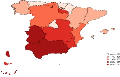
Figure 1 and 2 show the geographical distribution of the Spatial EBLUP estimates based on a distance approach for both HCR and S80/S20 indices. It can be observed that the southern regions of Spain show the highest percentage of poor individuals. In the left corner of the image the islands Ceuta, Melilla and Canarias are reported widely.

18

Figure 1. HCR spatial EBLUP estimates. Spain 2011

Figure 2. S80/S20 spatial EBLUP estimates. Spain 2011

Comparing Figure 1 with Figure 2, we can observe that, generally, those regions showing high values of HCR also present high values of S80/S20 index; this confirms that relative

poverty and inequality are generally correlated. On one hand, Madrid is an exception, since a low HCR is accompanied by a high level of inequality. On the other hand Melilla is a region with a high value of poverty and very little inequality.

By looking at the estimates spatial autoregressive coefficients it can be observed that, in both cases, this is lower when considering a distance threshold approach. In fact, the distance threshold is taken to guarantee at least one linkage for each area apart from the Canarias Islands. By doing this, most linkages between areas are found in northern Spain where we find rich (unequal) and poor (equal) regions. This can be understood by looking at Figure 3.

Each area is linked to its neighbours by means of black lines visible in the figure. Obviously the neighbouring structure is influenced by the approach followed by the researcher. In the figure we follow a distance based approach, that is two areas are called neighbours if the distance from each other is less than a threshold (taking as reference the centroid of each area as already explained in Section 3.1).

Figure 3. Distance threshold neighbours

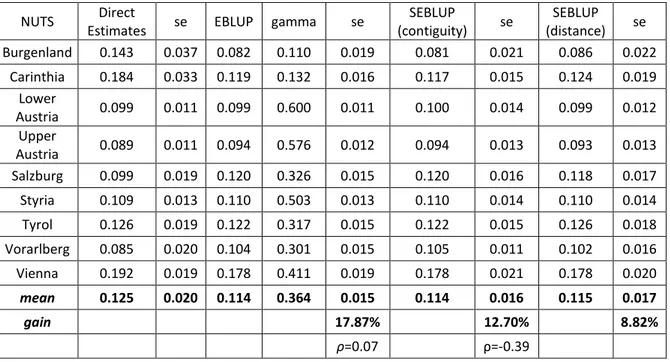
Tables 6 and 7 show instead direct, EBLUP and Spatial EBLUP estimates. It is interesting to compare here the performance of the model based estimators proposed with respect to the available sample size for each small area. It is expected that the gain in efficiency by adopting the EBLUP (or SEBLUP) estimator will be higher for those areas where the sample size is lower or where the estimated relative standard error is high. Table 6

20

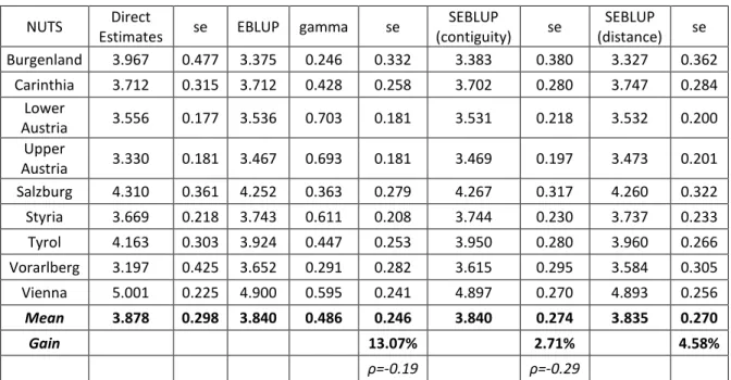
shows the results for the HCR Index. In the states of Burgenland and Carinthia the shrinkage factors are much lower than the others, meaning that most weight is attached to the regression synthetic estimator. It is not surprising that these areas show few sample sizes as well as a high estimated relative standard error, respectively 26% and 18%. Here model-based estimates are much lower than direct ones. The estimates of the spatial autoregression coefficients are moderate and the highest gain in efficiency is obtained with EBLUP. This suggests that if the spatial dependence is weak then it is better to use the traditional EBLUP. The results for S80/S20 Index show that for the areas of Burgenland and Vorarlberg the most weight is attached to the regression estimator while for Lower Austria the most weight is given to direct estimate. This is consistent with the expected results as the first two areas show low sample size and an estimate of the relative standard error of 14% and 11% respectively. On the contrary, high sample size is found in Lower Austria apart from a very low estimate of the relative standard error (4%). The Spatial EBLUP estimator leads to a very reduced gain in efficiency. This may be due to the fact that the estimated coefficient of spatial autoregression is moderate and negative, in the HCR case as well.

Table 6. HCR Estimates. Austria 2011

NUTS Direct

Estimates se EBLUP gamma se

SEBLUP (contiguity) se SEBLUP (distance) se Burgenland 0.143 0.037 0.082 0.110 0.019 0.081 0.021 0.086 0.022 Carinthia 0.184 0.033 0.119 0.132 0.016 0.117 0.015 0.124 0.019 Lower Austria 0.099 0.011 0.099 0.600 0.011 0.100 0.014 0.099 0.012 Upper Austria 0.089 0.011 0.094 0.576 0.012 0.094 0.013 0.093 0.013 Salzburg 0.099 0.019 0.120 0.326 0.015 0.120 0.016 0.118 0.017 Styria 0.109 0.013 0.110 0.503 0.013 0.110 0.014 0.110 0.014 Tyrol 0.126 0.019 0.122 0.317 0.015 0.122 0.015 0.126 0.018 Vorarlberg 0.085 0.020 0.104 0.301 0.015 0.105 0.011 0.102 0.016 Vienna 0.192 0.019 0.178 0.411 0.019 0.178 0.021 0.178 0.020 mean 0.125 0.020 0.114 0.364 0.015 0.114 0.016 0.115 0.017 gain 17.87% 12.70% 8.82% ρ=0.07 ρ=-0.39

Table 7. S80/S20 Index. Austria 2011

NUTS Direct

Estimates se EBLUP gamma se

SEBLUP (contiguity) se SEBLUP (distance) se Burgenland 3.967 0.477 3.375 0.246 0.332 3.383 0.380 3.327 0.362 Carinthia 3.712 0.315 3.712 0.428 0.258 3.702 0.280 3.747 0.284 Lower Austria 3.556 0.177 3.536 0.703 0.181 3.531 0.218 3.532 0.200 Upper Austria 3.330 0.181 3.467 0.693 0.181 3.469 0.197 3.473 0.201 Salzburg 4.310 0.361 4.252 0.363 0.279 4.267 0.317 4.260 0.322 Styria 3.669 0.218 3.743 0.611 0.208 3.744 0.230 3.737 0.233 Tyrol 4.163 0.303 3.924 0.447 0.253 3.950 0.280 3.960 0.266 Vorarlberg 3.197 0.425 3.652 0.291 0.282 3.615 0.295 3.584 0.305 Vienna 5.001 0.225 4.900 0.595 0.241 4.897 0.270 4.893 0.256 Mean 3.878 0.298 3.840 0.486 0.246 3.840 0.274 3.835 0.270 Gain 13.07% 2.71% 4.58% ρ=-0.19 ρ=-0.29

Figures 4 and 5 show Spatial EBLUP estimates based on a contiguity approach for HCR and S80/S20 in Austria. It can be observed that here areas with high values of HCR show also high values of S80/S20 and viceversa.

22

Figure 4. Spatial EBLUP estimates. S80/S20 Index. Austria

4. Discussion and concluding remarks

In this paper we have addressed the problem of estimating measures of well-being on their “regional dimension”; if fact, we have presented and compared two small area techniques, namely the cumulation and the spatial EBLUP (SEBLUP), on the basis of EU-SILC data from Austria and Spain. Both methodologies have been analysed observing both advantages and drawbacks.

In general, estimates computed with the cumulation method show standard errors which are smaller than those computed with EBLUP or SEBLUP. The gain of pooling SILC data over three years is therefore relevant, and may allow researchers to prefer this method. However, we would like to emphasise a point of great practical concern. Assessment of sampling precision of the estimates, taking into account the actual structure of the SILC sample, on which the data are based, has an essential requirement: provision of codes describing the sample in the survey micro data itself, along with accompanying documentation describing the design and the code. Inadequate (or sometimes even absence of) information on sample structure in survey data files is a long-standing and persistent problem in estimation from sample surveys. Unfortunately, even outstanding and highly standardised multi-country surveys such as EU-SILC have this sort of shortcomings, as underlined in this paper. A second drawback of the cumulation approach consists in the loss of the reference period to which the estimated measures coming from the data pooling are anchored. For example, in our exercise which is the reference year? 2010, which is the middle year, or 2011, which is the last available year (and comparable with SEBLUP estimates)? The debate on this issue is still open, and the present paper would intend to be a new starting point in this debate. On the other hand, when considering techniques such EBLUP and SEBLUP, some features of the areas for which new estimates are needed should be properly taken into account; first of all, the presence of islands or other types of geographical barriers; may be that some computational procedures would fail in the presence of such a situation. In such cases, the problem needs to be addressed adequately. The analysis may be restricted to those areas having at least one linkage with another and at the same time leaving the remaining as separate cases (this is usually done in the US with Alaska and Hawaii). If the spatial dependence is not an essential feature of data, meaning an estimated spatial autocorrelation coefficient nearly equal to zero, then a possible solution could be that of adopting the traditional EBLUP estimator. This estimator, by assuming the independence of the area-level random effects, does not suffer from spatial boundaries and, consequently, it is not sensitive to whether a region is an island or not. Obviously, this kind of problem can be easily overcome by following a design-based approach to small area estimation as in the case with the cumulation of estimates.

24

On the other hand, the fact that in the presented results the cumulation method performs better than EBLUP and SEBLUP should be judged taking into account an additional issue: when choosing the set of regressors in the EBLUP or SEBLUP, in general researchers do not have full access to information (regressors) present at area level. From this point of view, National Statistical Offices could in general perform better, having the possibility to access a large set of regressors.

Finally, we want to highlight that in the paper the estimation of the MSE of the SEBLUP estimator has been carried out by following a procedure which considers the analytical approximation of the MSE itself. Other estimators based on bootstrap procedures have been developed (see for instance Molina, Pratesi and Salvati, 2009). We have tried to apply these procedures; however, results have been unsatisfactory and some computational issues have been raised. Again, this is another aspect which future research should be focused on.

References:

Atkinson, A., Cantillon, B., Marlier, E., Nolan, B. (2002), Social Indicators: The EU and social inclusion. Oxford: Oxford University Press.

Banerjee, S., Carlin, B.P., Gelfand, A.E. (2004), Hierarchical modeling and analysis for spatial data. Chapman & Hall, New York.

Battese, G.E., Harter, R.M., Fuller, W.A. (1988), An error-components models for prediction of county crop areas using survey and satellite data, Journal of the American Statistical Association, 83, pp. 1–27.

Betti, G., Gagliardi, F., Lemmi, A., Verma, V. (2012), Sub-national indicators of poverty and deprivation in Europe: methodology and applications, Cambridge Journal of Regions, Economy and Society, 5(1), pp. 149-162.

Bivand, R.S., Rubio, V.G., Pebesma, E.J. (2008), Spatial analysis with R. Use R!. New York: Springer.

Cliff, A., Ord, J.K., (1981), Spatial processes. Models and applications. London: Pion. Cressie, N. (1993). Statistics for Spatial Data. New York: Wiley.

Elbers, C., Lanjouw, J.O., Lanjouw, P. (2003), Micro-level Estimation of Poverty and Inequality. Econometrica, 71, pp. 335-364.

European Commission (2010), Communication from the Commission. Europe 2020. A strategy for smart, sustainable and inclusive growth. Brussels, 3.3.2010 COM(2010) 2020.

Fay, R.E., Herriot, R.A. (1979), Estimates of income for small places: an application of James-Stein procedures to census data. Journal of the American Statistical Association, 74, pp. 269-277.

Foster, J.E., Greer, J., Thorbecke E. (1984), A class of decomposable poverty measures, Econometrica, 52, pp. 716-766.

Gosh, M., Rao, J.N.K. (1994), Small Area Estimation: An Appraisal (with discussion), Statistical Science, 9(1), pp. 55-93.

Handerson, C.R. (1950), Estimation of Genetic Parameters, Annals of Mathematical Statistics, 21, pp. 309-310.

Lohr, S.L. and Rao, J.N.K. (2000), Inference from dual frame surveys, Journal of American Statistical Association, 95, pp. 271-280.

Molina, I., Salvati, N., Pratesi, M. (2009), Bootsrap for estimating the MSE of the Spatial EBLUP, Computational statistics, 85, pp. 163-171.

Pratesi, M., Salvati, N. (2007), Small Area Estimation: The EBLUP model based on spatially correlated random effects. Statistical Methods and Applications, 17(1), pp. 113-141.

O’Muircheataigh, C., Pedlow, S. (2002), Combining samples vs. cumulating cases: a comparison of two weighting strategies in NLS97. American Statistical Association Proceedings of the Joint Statistical Meetings, pp. 2557-2562.

Rao, J.N.K (2003), Small Area Estimation. Wiley, London.

Verma, V. (2004), Sampling errors and design effects for poverty measures and other complex statistics. In: Proceedings of the VII international meeting quantitative methods for applied sciences: sampling designs for environmental, economic and social surveys: theoretical and practical perspectives, Siena.

Verma, V., Betti, G. (2011), Taylor linearization sampling errors and design effects for poverty measures and other complex statistics, Journal of Applied Statistics, 38(8), pp. 1549-1576.

Verma, V., Betti, G., Gagliardi, F. (2010), An assessment of survey errors in EU-SILC, Eurostat Methodologies and Working Papers, Eurostat, Luxembourg.

Verma, V., Gagliardi, F., Ferretti, C. (2013), Cumulation of poverty measures to meet new policy needs, in Advances in Theoretical and Applied Statistics. Torelli, N. and Pesarin, F.; Bar-Hen, Avner (Eds.) 2013, XIX, Springer.

Wells, J.E. (1998), Oversampling through households or other clusters: comparison of methods for weighting the oversample elements, Australian and New Zeeland Journal of Statistics, 40, pp. 269-277.