Seismic Assessment and Rehabilitation of existing RC Buildings not designed to withstand earthquakes

(1)

Buildings not designed to

withstand earthquakes

A thesis submitted for the degree of Doctor of Philosophy

Giuseppe Occhipinti

Supervisor:

Prof.Ivo Caliò - University of Catania Co-Supervisors:

Prof. Bassam Izzuddin - Imperial College of London Prof. Lorenzo Macorini - Imperial College of London

Coordinator:

Prof. Massimo Cuomo - University of Catania

«Assessment and Mitigation of Urban and Territorial Risks» XXIX Study Cycle

Department of Civil and Environmental Engineering University of Catania

(2)

(3)

Declaration

This submission is my own work. Any quotation from, or description of, the work of others is acknowledged herein by reference to the sources, whether published or unpublished.

The copyright of this thesis rests with the author and is made available under a Creative Commons Attribution Non-Commercial No Derivatives licence. Researchers are free to copy, distribute or transmit the thesis on the condition that they attribute it, that they do not use it for commercial purposes and that they do not alter, transform or build upon it. For any reuse or redistribution, researchers must make clear to others the licence terms of this work.

Giuseppe Occhipinti July 2017

(4)

(5)

Abstract

This thesis is focused on the seismic vulnerability assessment of existing multi-storey reinforced concrete buildings that were not designed to withstand earthquakes and on the identification of possible retrofitting strategies adoptable for their structural rehabilitation.

A typical ten-storey building has been identified as representative cases study of many similar buildings built in Catania (Sicily, south of ITALY) between the 60’s and 80’s before the introduction of a national seismic code in 1981. Since the building has been designed with reference to vertical loadings only it allowed the simple identification of further eight buildings characterised by different number of storeys, from nine to two, but maintaining the same plan layout.

Aiming at obtaining rigorous results and to validate the standard adopted procedures with those obtained by rigorous detailed simulations, the seismic assessment of the investigated buildings, before and after the proposed retrofitting measures, have been performed. For this purpose, advanced numerical models characterised by different modelling capabilities and computational demands have been implemented. The seismic vulnerability assessments, consistent to the current European Code prescriptions, have been performed by using the research version of the computer code 3DMacro that allows performing nonlinear push-over analyses by considering the important contribution of the non-structural infill panels. The detailed nonlinear analyses have been performed by means of high fidelity realistic models implemented in the advanced nonlinear FEM software ADAPTIC that allows performing full nonlinear static and dynamic analyses accounting explicitly for material and geometric nonlinearity. Moreover, according to a powerful partition modelling strategy and the capabilities of the parallel calculus, ADAPTIC makes possible the implementation of mathematical model of structures with a huge amount of details. The interaction between concrete frames and non-structural unreinforced hollow brick masonry infills has been evaluated by means of a FEM ad hoc implementation of the planar discrete macro-element, already implemented in 3DMacro within a discrete element framework. The original non-trivial implementation of the discrete macro-element in the FEM code ADAPTIC represents a significant original contribution of the present thesis. The large displacements capabilities of the software ADAPTIC has also empowered a new original research investigation that relates the investigation of progressive collapse scenarios due to local failures

(6)

vi

trigged by low, or moderate, earthquake actions on mid-rise weak reinforced concrete existing structures.

The thesis is divided into seven main chapters.

The first Chapter focuses the seismicity of the east coast of Sicily with major attention at the city of Catania. The second Chapter introduce the progressive collapse phenomena and it is preparatory to the investigation of the robustness of existing buildings designed for vertical loads only as possible consequence of moderate earthquake actions. The third Chapter investigates and discusses numerical simulations of an experimental test on progressive collapse of concrete frame structures already reported in literature. Several parametric analyses based on different nonlinear models have been performed with the aim of evaluating the influence of material parameters on the collapse response of typical reinforced concrete frames not designed to withstand earthquakes. In the fourth Chapter an original FEM implementation of a plane-discrete-macro-element is proposed aiming at modelling the non-structural infills in the nonlinear ADAPTIC models. The fifth Chapter describes the chosen case study and reports code-consistent parametric evaluations of seismic vulnerability of low- and mid-rise reinforced concrete buildings. The case study has been defined according to a simulated design that was based on the survey of existing residential buildings designed and built in Catania between the 60’s and 80’s and on the design code that the engineers adopted in those decades. In this preliminary evaluation, only push-over analyses have been performed with the computer code 3DMacro that empowers a reliable model of non-structural masonry panels. Starting from the definition and design of the case study ten-storey building, other eight structures have been obtained. Moreover, the results are expressed for different soil conditions according to the Italian 2008 technical code. Chapter sixth considers the seismic vulnerability evaluation of the ten storeys case-study by means of a realistic model implemented in ADAPTIC considering the ribbed slabs and the infilled masonry panels contributions. The detailed FEM implementation of the plane macro-element is adopted to model the non-structural walls. The non-linear dynamic response of the two models are compared and discussed underling the unreinforced clay walls contribution. The thorough vulnerability assessments have been performed according to nonlinear dynamic analyses considering both material and geometrical nonlinearities.

The possible retrofitting strategies of the ten-storey building are discussed in Chapter 7. The proposal is the results of the research project that has been financed by ANCE|Catania and developed by a research

(7)

team coordinated by Prof. I.Caliò and Prof. B.Izzuddin. The retrofitting strategy consists in an innovative structural perimetral steel skeleton made by a synergetic combination of centred braced frames and eccentric bracing system endowed with dissipative shear links. The proposed solution has been investigated by means of a high fidelity model implemented in the software ADAPTIC

The numerical results obtained from the high fidelity 3D nonlinear dynamic simulations showed a very poor seismic performance of the existing structure. The results of numerical simulations for the retrofitted structure confirm that the proposed solution significantly enhances the response under earthquake loading, allowing the structure to resist the design earthquake with only limited damage in the original RC beams and columns, highlighting the feasibility of retrofitting for this typical multi-storey RC building structure.

Keywords: Infill frame, Robustness, Seismic vulnerability, Existing RC buildings, Macroelement, High Fidelity Model.

(8)

(9)

Acknowledgments

I would like to express my sincere gratitude to my advisor Prof. Ivo Caliò for his priceless continuous support of my Ph.D. He guided and motivated me to get better results, not only for this thesis. I cannot fail to thanks him for his thorough review of the final manuscript. He profoundly supported me and acted as a mentor of immense knowledge.

I would like to express my special appreciation and thanks to Prof. Bassam A. Izzuddin for his immense support and his inestimable guideless. He gave me the opportunity to join his Computation Structural Mechanics group at Imperial College of London and let me to use ADAPTIC for my thesis.

My sincere thanks also goes to Prof. Lorenzo Macorini, he encouraged and motivated me. He had also a central role with its thorough reviews of articles and of the final manuscript of this thesis.

I am in debt with ANCE|Catania, the former president Nicola Colombrita and the president Giuseppe Piana. Under their guide, ANCE|Catania believed in the research, financed my scholarship and the related researches. No one of the results that have been achieved would have been obtained without their enlightened presidency.

I am also grateful to Ph.D. Francesco Cannizzaro for his stimulating observations on my results and to Ph.D. Davide Rapicavoli for his support in the definition of graphical user interface input/output facilities.

I would like to thank Ph.D. Carlos Escobar Del Pozo and Prof. Paulo Marcos Aguiar, good friends are rare but London gave me other two.

Finally, I reserve a special thanks to my family and my beloved Angela because no houses can be built on the sand no lives can be lived without true love.

(10)

(11)

xii

4.2.1 Single strut model 106

4.2.2 Multi Diagonal Struts Models 107

4.2.3 Crisafulli and Carr Model (2007) 108

4.2.4 Hashemi and Mosalam – SAT Model (2007) 109

4.2.5 Kadyesiewski and Mosalam Model (2009) 110

4.2.6 Mohebkhah et al. MTS Model (2007) 112

4.2.7 Caliò et al. a two-dimensional MacroElement 113

4.3 An original FEM implementation of the MacroElement 115

4.3.1 The kinematics of the infilled macro-element 116

4.3.2 Mechanical response 127

4.4 Calibration procedures 130

4.4.1 Axial/Flexural calibration 130

4.4.2 Sliding Calibration 132

4.4.3 Shear diagonal behaviour 134

4.5 Reliability of the proposed Macro-Element 137

4.5.1 Parametric analysis 143

4.5.2 Numerical validation of the implemented macro-element 154

CHAPTER 5.

Seismic vulnerability parametric analyses 156

5.2 The typical building 159

5.3 Parametric model 164

CHAPTER 6.

High fidelity assessment 190

6.2 Realistic FEM model 193

6.3 Non Linear Dynamic Analyses 199

6.4 Seismic and Robustness Assessment 199

CHAPTER 7.

Proposed retrofitting strategy 225

7.2 Literature Review 229

7.3 The proposed eccentric bracing system 235

7.4 The retrofitted case study 245

CHAPTER 8.

Conclusions 262

8.1 Summary 264

8.1 Some consideration on the achieved results and possible future developments 270 CHAPTER 9. Bibliography 275 CHAPTER 10. Appendices 285 APPENDIX I.

Ductile Mechanisms: Chord Rotation Capacity 287

I. Eurocode-8: part3 289

II. Italian NTC08 294

III. Ductile Mechanisms: Chord Rotation Demand 295

(13)

Brittle Mechanisms: Shear Capacity 300

I. Eurocode 8 302

II. Italian Seismic Code 303

III. Biaxial Shear 305

APPENDIX III.

Parametric Models 307 APPENDIX IV.

(14)

(15)

List of Tables

Table 1-1 Target Spectrum ... 20

Table 1-2 Main characteristics of the seven adopted records ... 21

Table 2-1 Loads and Analyses ... 47

Table 3-1 Material Properties ... 57

Table 3-2 CON1 properties ... 63

Table 3-3 Modified Kent and Park [61]. ... 63

Table 3-4 SLT1 properties ... 65

Table 3.5 Values of the compressive strength ... 66

Table 3.6 Variation of second tensile elastic modulus ... 69

Table 3.7 Values of the Lateral Restrains Stiffness ... 71

Table 3.8 Geometry properties of the structural elements... 79

Table 3.9 SLT1 properties ... 80

Table 4-1 Variation of softening shear modulus ... 143

Table 4-2 Variation of shear ultimate strength ... 145

Table 4-3 Variation of tensile softening modulus ... 147

Table 4-4 Variation of sliding shear strength ... 149

Table 4-5 Variation of sliding elastic modulus ... 151

Table 4-6 Materials properties ... 154

Table 5-1 Columns cross-sections ... 161

Table 5-2 Characterization of concrete materials ... 163

Table 5-3 Characterization of steel materials ... 163

Table 5-4 Mechanical parameters of masonry walls ... 164

Table 5-5 (Colour) Modal calibration of the 3DMacro bare model ... 166

Table 6-1 Concrete materials for the dynamic analysis of the frames ... 195

Table 6-2 Steel materials for the dynamic analysis of the frames ... 195

Table 6-3 Steel materials for the dynamic analysis of the frames [89] ... 197

Table 6-4 Maximum drifts determined by the BF and IF models ... 204

Table 7-1 Maxima Drifts Demands... 258

(16)

(17)

List of Figures

Figure 1.1 Graphical representation of the Risk function. ... 4

Figure 1.2 (Colour) a) European population density 2010/2011, b)European Seismic Hazard Map (ESHM13) displaying the 10% exceedance probability in 50 years for peak ground acceleration (PGA) in units of gravity (g ). ... 5

Figure 1.3 (Colour) Detail of the Seismic Hazard map of Europe. ... 6

Figure 1.4 (Colour) Detail of the population density map ... 6

Figure 1.5 Civil victims in the XX century in Italy due to earthquakes or global war. ... 7

Figure 1.6 “Casa baraccata” (1783) ... 7

Figure 1.7 The first Italian Seismic Hazard Map. Prof. Torquato Taramelli, 1888 ... 8

Figure 1.8 “Progetto Finalizzato Geodinamica” CNR (1976-1981)... 9

Figure 1.9 Italian hazard map in 1984 and seismic categories ... 10

Figure 1.10 (Colour) Proposed Hazard map of Italy in 1996 ... 11

Figure 1.11 Comparison between the adopted map in 1997 (a) and the proposed map of the 1998. As the star shows the Molise earthquake struck a not classified area. ... 11

Figure 1.12 Map of 1998 (“Proposta 98”) and the map of 2003 based on it. ... 12

Figure 1.13 (Colour) Actual Hazard map of Italy. (April 2004) ... 13

Figure 1.14 Tectonic framework of the study area with major structural domains of southern Italy and active faults identified through surface geological evidence ... 14

Figure 1.15 Tectonic sketch and Epicentral map of the regional earthquakes. ... 15

Figure 1.16 Ancient figuration of the 1669 eruption ... 16

Figure 1.17 The 1693 Earthquake in an ancient picture. ... 17

Figure 1.18 Spectrum compatibility area in the Italian Seismic code ... 19

Figure 1.19 (Colour) Disaggregation in terms of Magnitude and Epicentral Distance for a Return Time of 475 year related to a Vt of 50 years and a soil type D (SLC. Soil D. Category T1) ... 21

Figure 1.20 (Colour) Planar spectrum compatibility ... 22

Figure 1.21 (Colour) Vertical spectrum compatibility ... 22

Figure 1.22 (Colour) Flowchart of the procedure for defining the accelerograms ... 23

Figure 1.23 (Colour) Planar and vertical spectrum compatibility ... 23

Figure 1.24 Seven accelerograms and their three components ... 25

Figure 2.1 Growth of number of publications between 1964 and 2016 (scopus.com) ... 29

Figure 2.2 Tie Forces in a Frame Structure ... 31

Figure 2.3 Ronan Point Building a) scheme of the collapse b) global view c) details ... 33

Figure 2.4 Murrah Federal Office Building [1995] a) helicopter view, b) frontal view ... 33

Figure 2.5 Collapse of the World Trade Center NY City [2001] ... 34

Figure 2.6 Static bending moments (My) in a framed structure [39] ... 35

Figure 2.7 Collapse bending moments (My) in a framed structure [39] ... 35

Figure 2.8 Plan of San Diego Hotel and blew up columns (crosses) [60] ... 36

Figure 2.9 (Colour) Direction of principal stresses and Plastic strain of the bars and compressed area. ... 37

Figure 2.10 (Colour) Principal Tensions Map... 37

Figure 2.11 Tensile forces transferring through stirrups [44]... 38

Figure 2.12 Sketch of the steel frame building [27] ... 40

Figure 2.13 Sub structural levels for progressive collapse assessment ... 41

Figure 2.14 Sudden column event with gravity load Po [26]: (a) actual event; (b) step load dynamic idealization; (c) static analysis using amplification factor λd ... 42

Figure 2.15 Collapse modes due to column loss in steel (a) and RC (b) frames ... 43

Figure 2.16 Qualitative representation of the B.Izzuddin's energetic approach. ... 43

Figure 2.17 Timeline of collapse event and national regulation [47] ... 45

Figure 2.18 Applicability flowchart [33]. ... 46

(18)

xviii

Figure 2.20 Loads and Load Locations for External and Internal Column [31] ... 48

Figure 2.21 Strategies for Accidental Design Situations ... 49

Figure 2.22 Recommended limit of admissible damage ... 50

Figure 3.1 3D Numerical Model in LUSAS ... 57

Figure 3.2 Two-storey RC frame specimen with beams with discontinuous longitudinal reinforcement ... 58

Figure 3.3 Tearing out of the stirrups is evident in the second level beam. [46] ... 59

Figure 3.4 Experimental responses of the RC frame subjected to column loss. ... 59

Figure 3.5 Numerical model in ADAPTIC. ... 60

Figure 3.6 Local reference system and element forces for cbp2 element. ... 60

Figure 3.7 Longitudinal reinforcement bars and FEM discretization ... 61

Figure 3.8 ADAPTIC fibre section types adopted in the finite element model: a)RCCS; b) RCTS. [63] ... 62

Figure 3.9: ADAPTIC CON1 model ... 63

Figure 3.10 Modified Kent and Park [61]. ... 63

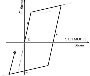
Figure 3.11 ADAPTIC STL1 model and model material parameters. ... 65

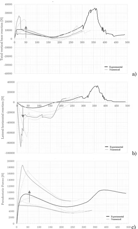
Figure 3.12 Influence of Compressive Strength fc in a) Static Responses, b) Horizontal reaction, c) Pseudostatic Assessment ... 68

Figure 3.13 Influence of Second Tensile Elastic Modulus Et2 in a) Static Responses, b) Horizontal reaction, c) Pseudostatic Assessment ... 70

Figure 3.14 Influence of Lateral Restrains Stiffness in a) Static Responses, b) Horizontal reaction, c) Pseudostatic Assessment ... 72

Figure 3.15 Best-fitting curve in nonlinear static response... 73

Figure 3.16 Best-fitting curve in the Pseudostatic response ... 74

Figure 3.17 Schematic behaviour of a light reinforced concrete beam in a column loss event. ... 75

Figure 3.18 Superimposing of the experimental response and the Adaptic response. ... 76

Figure 3.19 (Colour) Configuration of the concrete beam near the last peak value. The hatched area represents the concrete cover crushing. ... 76

Figure 3.20 Static nonlinear response of three models. ... 78

Figure 3.21 3D representation of the concrete frame building ... 81

Figure 3.22 Plan view ... 81

Figure 3.23 2D concrete bare frame, scale 1:1 ... 82

Figure 3.24 Model A: two floor, six bay frame; Model B: three store and six bay frame; Model C: six storey and six bay frame; Model D: ten storey and six bay frame ... 82

Figure 3.25 Static responses ... 83

Figure 3.26 Pseudostatic responses ... 83

Figure 3.27 Diagrams of the shear forces variation in MODEL A ... 85

Figure 3.28 Diagrams of the shear forces variation in MODEL B ... 85

Figure 3.29 Diagrams of the shear forces variation in MODEL C ... 86

Figure 3.30 Diagrams of the shear forces variation in MODEL D ... 86

Figure 3.31 Comparison of the Bending Moments My in the first floor beam ... 87

Figure 3.32 Comparison of Bending Moments My in the second floor beam ... 87

Figure 3.33 Comparison of Shear Forces Vz in the first floor beam ... 88

Figure 3.34 Comparison of Shear Forces Vz in the second floor beam ... 88

Figure 3.35 FE discretisation and monitored section (red) ... 89

Figure 3.36 Push Down Curves and significant points ... 89

Figure 3.37 Collapse Shape after E point ... 90

Figure 3.38 Sketch of the Fibre elements discretisation. ... 91

Figure 3.39 Detail of the one-way spanned ribbed slab ... 92

Figure 3.40 General view of the FEM 3D high fidelity model ... 92

Figure 3.41 Extruded view of the detail of concrete slabs system. ... 92

Figure 3.42 (Color) Assignment of sections in concrete frames ... 93

Figure 3.43 FEM Model of a generic high fidelity floor model. Model A ... 94

(19)

Model C. ... 94

Figure 3.46 Deformed shape ... 95

Figure 3.47 Typical deformation modes due to column loss in steel (a) and RC (b) frame structures. ... 96

Figure 3.48 Push Down Curve Model A ... 96

Figure 3.49 Push Down Curves of the three FEM floor models ... 97

Figure 3.50 Pseudostatic Curve ... 98

Figure 3.51 (Colour) Detail of Concrete slab stresses, x [MPa], a) top, b) bottom ... 99

Figure 3.52 (Colour) Detail of Concrete slab stresses, y [MPa] a) top, b) bottom ... 100

Figure 3.53 (Colour) Reinforcement tensile stresses, x andy [MPa] ... 101

Figure 4.1 Failure modes for one storey single-bay infilled r.c. frames a) Corner crushing b) Compressed strut crushing c-d) Knee-braced e) Shear Sliding [69] ... 106

Figure 4.2 Single Strut Model Scheme ... 107

Figure 4.3 Few strut models: (a) Schimidt (b) Chrysostomou, (c) Crisafulli ... 107

Figure 4.4 Knee Frame Model [74]... 108

Figure 4.5 Crisafulli-Carr model [76] ... 108

Figure 4.6 Variation of Area [76] ... 109

Figure 4.7 Strut and tie model (Hashemi and Mosalam 2007) ... 110

Figure 4.8 Strut and tie model (Kadyesiewski and Mosalam 2009) ... 111

Figure 4.9 Interaction domain [78] ... 112

Figure 4.10 The basic macro-element: (a) undeformed configuration; and (b) deformed configuration. ... 113

Figure 4.11 . Main in-plane failure mechanisms of a masonry portion: (a) flexural failure; (b) shear-diagonal failure; and (c) shear-sliding failure ... 114

Figure 4.12 . Simulation of the main in-plane failure mechanisms of a masonry portion by means of the macro-element: (a) flexural failure; (b) shear-diagonal failure; and (c) shear sliding failure ... 114

Figure 4.13 Proposed macroelement ... 116

Figure 4.14 Location and the corresponding orientation of the degrees of freedom in the global system ... 117

Figure 4.15 Relationship between local and global degrees of freedom in the external edges... 117

Figure 4.16 Relationship between local and global degrees of freedom in the internal edges. ... 120

Figure 4.17 STMDL47 Cyclic material model ... 130

Figure 4.18 Schematic representation of the fibre discretisation ... 131

Figure 4.19: ADAPTIC STL1 model and model material parameters. ... 133

Figure 4.20 Representation of the fibre discretisation and sliding calibration ... 134

Figure 4.21 Homogenised equivalence for the shear springs calibration [65] ... 136

Figure 4.22 STMDL47 Cyclic material model ... 136

Figure 4.23 Bare Frame Model ... 138

Figure 4.24 (Colour) Collapse shape of the bare frame specimen [49] ... 139

Figure 4.25 Bare Frame Response curve ... 139

Figure 4.26 Infilled Frame Models synthetic description: left side, specimen with openings [50]; right side, specimen with full eight walls [49] ... 140

Figure 4.27 Structural cross-sections and bricks dimensions [49]. ... 140

Figure 4.28 Full-height Infill Frame structural response ... 141

Figure 4.29 Scheme of the FEM model ... 142

Figure 4.30 Influence of the Shear Model Softening Modulus ... 144

Figure 4.31 Detail of the diagram on the Influence of the Shear Model Softening Modulus ... 144

Figure 4.32 Influence of the Shear Ultimate Strength ... 146

Figure 4.33 Detail of the diagram on the Influence of the Shear Ultimate Strength ... 146

Figure 4.34 Influence of Tensile Softening Modulus ... 148

Figure 4.35 Detail of the Influence of Tensile Softening Modulus ... 148

Figure 4.36 Influence of Sliding Ultimate Strength ... 149

Figure 4.37 Detail of the diagram on the Influence of Sliding Ultimate Strength ... 150

(20)

xx

Figure 4.39 Parametric analysis on high subdivided panels ... 152

Figure 4.40 Numerical Model with 45 macroelements for each infilled panel ... 152

Figure 4.41 Numerical simulation of the full-height infill frame test. ... 153

Figure 4.42 (Colour) MODEL A – PushOver Capacity curves ... 155

Figure 4.43 (Colour) MODEL B – PushOver Capacity curves. ... 155

Figure 5.1 (Colour) CRESME 2012 based on ISTAT data in ITALY ... 158

Figure 5.2 Generic architectural (a) and structural (b) plan of the case study. ... 161

Figure 5.3 A three-dimensional view of the frame structure of the designed typical building. ... 162

Figure 5.4 Concrete Column cross section and reinforcement layouts (section 30x30 and 40x80)162 Figure 5.5 Example of reinforcement layout ... 163

Figure 5.6 (Colour) Similarities between numerical and real buildings ... 165

Figure 5.7 Comparison between the modal periods of the two models ... 170

Figure 5.8 Percent Period increment in the early three modes ... 170

Figure 5.9 3DMacro models of the ten storey building a) Bare Frame model b) Infill Frame model ... 171

Figure 5.10 Mass proportional capacity curves ... 172

Figure 5.11 Fundamental mode proportional capacity curves ... 173

Figure 5.12 Variation of capacity displacement due to infills contribute in mid-rise buildings. ... 174

Figure 5.13 Ten-storey models capacity curves in a) x and b) y direction for the Mass proportional loads distribution ... 175

Figure 5.14 Ten-storey models capacity curves in a) x and b) y direction for the Fundamental Mode proportional loads distribution ... 175

Figure 5.15 (Colour) Ten-storey models deformed shapes under mass proportional loads distribution: a) x and b) y direction for bare frame model and c) x and d) y direction for infill frame model. ... 176

Figure 5.16 (Colour) Ten-storey models deformed shapes under fundamental mode proportional loads distribution: a) x and b) y direction for bare frame model and c) x and d) y direction for infill frame model. ... 177

Figure 5.17 (Colour) Ten-storey models deformed shapes: a) x and b) y direction for bare frame model and c) x and d) y direction for infill frame model. ... 179

Figure 5.18 3DMacro a) Bare and b) Infill two-storey building ... 180

Figure 5.19 Increment of normalised base shear value thanks to infills for the two directions (Soil Category A) ... 181

Figure 5.20 Two-storey models capacity curves in a) x and b) y direction for the Mass proportional loads distribution ... 182

Figure 5.21 Two-storey models capacity curves in a) x and b) y direction for the Fundamental Mode proportional loads distribution ... 182

Figure 5.22 (Colour) Two-storey models deformed shapes under mass proportional loads distribution: a) x and b) y direction for bare frame model and c) x and d) y direction for infill frame model. ... 183

Figure 5.23 (Colour) Two-storey models deformed shapes under fundamental period proportional loads distribution: a) x and b) y direction for bare frame model and c) x and d) y direction for infill frame model. ... 184

Figure 5.24 Displacement Safety Factors (Soil Category A) ... 185

Figure 5.25 (Colour) Trend of the Safety Factors in terms of displacements (Demand/Capacity) 186 Figure 5.26 Average values of the Safety Factors increments ... 187

Figure 5.27 Variation of displacement safety factors according to different soil categories. ... 188

Figure 5.28 Variation of displacement safety factors according to different soil categories. ... 188

Figure 6.1 Sketch of the Fibre elements with nonlinear material models ... 194

Figure 6.2 Bare Frame 3D model in ADAPTIC a) geometric model; b) extruded computational model ... 194

Figure 6.3 Detail of the High Fidelity Model computational model ... 194

Figure 6.4 (Colour) Detail of the one way deck in the High Fidelity Model a) geometric model; b) computational model ... 195

(21)

structure, (b) and for the infilled one ... 197

Figure 6.7 Partition strategy with 31 partitions for the analysed building ... 199

Figure 6.8 Global response of the BF model for the seven accelerograms ... 200

Figure 6.9 Global response of the IF model for the seven accelerograms ... 201

Figure 6.10 Average drift values for the BF (.1) and IF (.2) model in the two planar (a, b) and vertical displacements (c) ... 202

Figure 6.11 (Colour) Detail of the column loss scenario during the NLDA5 analysis. ... 204

Figure 6.12 General interpretation of the Chord Rotation in Beam/Column Elements ... 205

Figure 6.13 Cyclic experimental results [98], numerical simulation and shear capacity assessment in agreement with Eurocode and NTC08. ... 206

Figure 6.14 Localization of first failures a) Shear failure b) Ultimate chord rotation ... 207

Figure 6.15 (Colour) Shear demand/capacity ratio for the BF model in the NLDA1 analysis. ... 209

Figure 6.22 (Colour) Chord rotation ratios for the BF model in the NLDA1 analysis. ... 213

Figure 6.29 (Colour) Shear demand/capacity ratio for the IF model in the NLDA1 analysis. ... 217

Figure 6.36 (Colour) Chord rotation ratios for the IF model in the NLDA1 analysis. ... 221

Figure 7.1 Publications on retrofitting strategies of existing structures [100] ... 227

Figure 7.2 (Colour) Acceleration-Displacement Response Spectrum (ADRS) illustration of different retrofit philosophies and strategies a) strengthening b) added damping c) base isolation d) partial SW (weakening only) e) full SW (weakening and further enhancement) [102]. ... 228

Figure 7.3 Steel Braced Frame ... 230

Figure 7.4 Hysteresis plot for buckling-restrained brace and concentric brace [105] ... 231

Figure 7.5 Shear wall retrofitting method ... 232

Figure 7.6 Steel Plate Shear Wall System ... 234

Figure 7.7 Flowchart of the new proposal identification... 235

Figure 7.8 Eccentric bracing systems [112]. ... 236

Figure 7.9 Generalised stresses due to a concentrated horizontal load ... 238

Figure 7.10 Generalised stresses due to a concentred vertical load... 239

Figure 7.11 Scheme of the proposed Eccentric Bracing System ... 240

(22)

xxii

Figure 7.13 Seismic vulnerability of the existing case study with and without infills and for four soil categories. ... 244 Figure 7.14 Planar scheme of the retrofit systems distribution ... 245 Figure 7.15 Front and back of the retrofitted structure ... 246 Figure 7.16 (a) 3D ADAPTIC model of the strengthened building, (b) modelling of an eccentric bracing with a dissipative shear link (deformed configuration) ... 247 Figure 7.17 Fundamental periods of the bare frame, infilled frame and retrofitted bare frame structures. ... 248 Figure 7.18 (Colour) Deformed shape and Displacements at the last step of the NLDA1 analysis. ... 250 Figure 7.19 (Colour) Deformed shape and Displacements at the last step of the NLDA6 analysis. ... 251 Figure 7.20 (Colour) Contours of Displacement history of the a) BF models and b) of the RIF models in NLDA1 analysis. ... 252 Figure 7.21 (Colour) Contours of Displacement history of the a) BF models and b) of the RIF models in NLDA6 analysis. ... 252 Figure 7.22 Displacements in Y direction of the a) BF and b) RIF models in NLDA1. ... 254 Figure 7.23 Displacements in X direction of the a) BF and b) RIF models in NLDA1. ... 254 Figure 7.24 Displacements in X direction of the a) BF and b) RIF models in NLDA6. ... 255 Figure 7.25 Displacements in Y direction of the a) BF and b) RIF models in NLDA6. ... 255 Figure 7.26 Drift demand of the a) BF and b) RIF models in NLDA1 ... 256 Figure 7.27 Normalized Drift Demand of the a) BF and b) RIF models in NLDA1 ... 256 Figure 7.28 Drift demand of the a) BF and b) RIF models in NLDA6 ... 257 Figure 7.29 Normalised Drift demand of the a) BF and b) RIF models in NLDA6 ... 257 Figure 7.30 Chord rotation ratios of all the concrete columns for NLDA1 analysis ... 260 Figure 7.31 Chord rotation ratios of all the concrete columns for NLDA6 analysis ... 260 Figure 7.32 Shear demand/capacity ratio of the concrete columns for NLDA1 analysis ... 261 Figure 7.33 Shear demand/capacity ratio of the concrete columns for NLDA6 analysis ... 261 Figure 10.1 Confined and unconfined parts over the cross-section and along member with (a) circular section and circular hoops; or (b) square section and multiple ties [116]. ... 290 Figure 10.2 Local dof of 3D elastic-plastic cubic beam [62] ... 296 Figure 10.3 Chord Rotation components ... 297 Figure 10.4 Generic architectural (a) and structural (b) plan of the case study. ... 317 Figure 10.5 RC Beams. ... 318 Figure 10.6 RC Columns Cross-Sections. ... 319

(23)

CHAPTER 1. C

ATANIA

’

S

EISMIC

H

AZARD

he interest of the scientific community on the seismic assessment and the vulnerability of concrete frame structures grew exponentially after the introduction of the national seismic codes. In Italy, it happened in 1974 with the introduction of a seismic code for great part of the Italian territory. At the end of the 90’s, several Italian university research groups were involved in a huge research project know as Catania Project focused on the assessment of the seismic risk of the city of Catania and more in general on the oriental area of Sicily. The Catania urban peculiarities and its high seismic risk, are well defined by the following words [1] “The building process that take place in Italy

after the World War II, and especially during the 50s and 60s, was characterised by concrete frame structures designed to resist only to gravity loads. Several Italian areas were defined prone regions after the latter period and, consequently, the study of those buildings is extremely interesting for the vulnerability assessment studies. From this point of view, the cold case Catania is hugely emblematic. The seismic assessment of the existing concrete frame buildings, which were designed to resist only to gravity loads, represents a highly relevant topic due to social and economic consequences, consistently with the huge number of similar building typologies in our Country […]”

(24)

(25)

1.1 _Background

The reinforced concrete frame buildings designed for vertical loads only are widespread in Italy and in a several Mediterranean countries. The thesis is focused on mid-rise buildings not designed to resist to earthquake loadings. A typical building that is representative of many similar structures built in Catania between the 60s and 80s, is considered as case study. Although it is assumed as a representative Catania middle-rise building, the obtained results can be extended to many similar buildings of different areas in the world that have been recently recognised seismic prone regions.

The structures that were built without seismic design methods are characterised by several structural weaknesses. In addition a natural degrade of the structural materials usually affects reinforced concrete structures in few years. These structural deficiencies affect and increase the seismic vulnerability and, consequently, the seismic risk. Furthermore, the seismic risk is a function of hazard, vulnerability and exposure in a specific area. Their meanings are explained below.

Seismic risk. It is defined as potential economic, social and

environmental consequence of hazardous events that may be occur in a determinate area in a specific period.

Seismic hazard. It is the probability that an earthquake occurs in a

geographic area, within a specific time span, and a ground motion intensity exceeding a threshold.

Seismic Vulnerability. It defines the condition resulting from physical,

construction processes, geometric and material properties of a structure and environmental factors or processes that increase its susceptibility to the impact of a hazard.

Exposure. It indicates the elements that are affected by natural

disasters (e.g. people and property).

Summarising, “risk” defines the expected value of losses (deaths, injuries, property, etc.) that a hazardous event may cause.

(26)

4

Figure 1.1 Graphical representation of the Risk function.

From an engineering point of view, the Figure 1.1 depicts the conventional and adopted strategy to reduce the Seismic Risk. The reduction of seismic vulnerability of existing structures not designed to withstand earthquakes decreases the Seismic Risk.

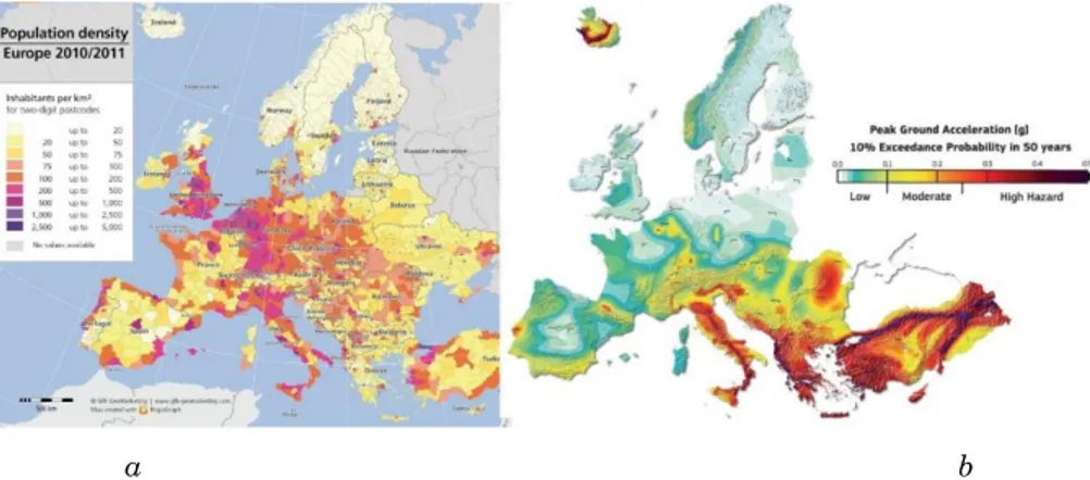
Several Mediterranean and European regions have been only recently defined seismic prone areas. Figure 1.2 visualises the previously described meanings of “hazard” and “exposure” comparing two meaningful maps. The first map (Figure 1.2.a) depicts the density of habitants in the European countries estimated in 2011. The latter map (Figure 1.2.b) reports the peak ground acceleration with the exceedance probability of 10% in a period of 50 years and the cold colours indicate comparatively low hazard areas (PGA≤ 0.1g ), yellow and orange indicate moderate-hazard values (0.1g). The comparison of the two colour maps underlines the strategic necessity of accurate evaluation of seismic vulnerability of existing buildings. In fact, by comparing the two images the higher level of population density are spread on the same areas with the higher expected peak ground accelerations.

(27)

a b Figure 1.2 (Colour) a) European population density 2010/2011, b)European

Seismic Hazard Map (ESHM13) displaying the 10% exceedance probability in 50 years for peak ground acceleration (PGA) in units of gravity (g ).

Even though it can be seemed irrational, several European cities with millenarian history are placed along the darker area of the hazard map. Cities like as Istanbul, Athens, and Tirana have an extremely high seismic hazard. On the other hand, the surrounding lands around these cities are characterised by a relative low population density. In this scenario, the Italian peninsula has a higher seismic risk. In fact, the population density map shows smaller cities but bigger areas characterised by the same density. Large areas, such as the Sicilian eastern cost, appear affected by unneglectable values of inhabitants per km2_{(200-500) and a high seismic hazard value (0.3-0.4g). Looking at}

Figure 1.3 and Figure 1.4, the high seismic risk of Sicily can be understand.

(28)

6

Figure 1.3 (Colour) Detail of the Seismic Hazard map of Europe.

Figure 1.4 (Colour) Detail of the population density map

Furthermore, the inadequacy and vulnerability of the existing buildings in that area make Sicily one of the European regions characterised by high seismic risk and one of the higher in the all over the World. Lastly, aiming to underline this extremely dangerous condition, the Figure 1.5 compares the civil victims during the World War II and those of earthquakes in the XX century in Italy. The victims died immediately in building collapses of few days later due to the severe injuries.

(29)

Figure 1.5 Civil victims in the XX century in Italy due to earthquakes or global war.

1.2 _{Seismic Hazard in Italy and Seismic Code}

evolution

Even though the seismic hazard of the Italian peninsula was seriously argued since the last decades of the 1800 by the academic researchers, Ferdinando IV Borbone of Kingdom of the Two Sicilies issued the first European Seismic Prescription in 1785. After the devastating earthquake that stroke the southern part of Italy on 5th February 1783, he issued a construction regulation that imposed an innovative construction technique, the “casa baraccata” (Figure 1.6). The construction method, which involved wooden frames and masonry infill panels, was applied in several towns and saved thousands life during the earthquakes of 1905 and 1908.

(30)

8

At the end of the 1800, the hazard map and the seismic classification were based on correlation between geological characteristics and historical earthquakes. In this way, Prof. Torquato Taramelli proposed a hazard map of the Italian peninsula in 1888, as Figure 1.7 shows. The map, the oldest in Italian seismology, described the seismic areas in terms of Mercalli scale effects. Taramelli worked for finding a correlation between the seismic areas and their geological properties, but he did not obtained evident correlations. On the other hand, it is notable that the map showed a seismic classification similar to the more modern hazard maps.

Figure 1.7 The first Italian Seismic Hazard Map. Prof. Torquato Taramelli, 1888

The first Italian Seismic Code that involved many peninsula areas was published in 1974 (law 64, 1974). The 1974 Building Code established the spectral horizontal design forces; but they were not explicitly related

(31)

to ground motion parameters. The local seismic coefficients were established according to some criteria and it was named “seismic classification”.

Figure 1.8 “Progetto Finalizzato Geodinamica” CNR (1976-1981)

The 1984 seismic classification of the Italian territory, still in use in 1997 and until the 2002, derived from the results of research group called “Progetto Finalizzato Geodinamica” funded from 1976 until 1981 by CNR ((Italian) National Council of Research).

(32)

10

Figure 1.9 Italian hazard map in 1984 and seismic categories

Figure 1.9 shows the seismic classification of the Italian peninsula in 1984. According to the results of the before mentioned research group, the land was subdivided in four categories. The fourth category characterised the not prone areas. In that period, the Eastern Sicilian cost was catalogued as II seismic category.

After the Umbria-Marche earthquake in 1997, the Commission for the Major Risks established a working group charged of updating the seismic classification of the Italian territory. The parameters that have been adopted in that project were:

_{Housner (1952; 1963) spectrum intensity}

_{H50 = 10% exc. probability in 50 years, 0.2-2 sec.}  H10 = 10% exc. probability in 10 years, 0.1-0.5 sec.  Maximum observed intensity

Unfortunately, the results of the study were not adopted until the 2002.

(33)

Figure 1.10 (Colour) Proposed Hazard map of Italy in 1996

In 2002 an earthquake struck Molise (a region in the mid of Italy) and an area that was not included in the seismic zonation was hit (Figure 1.11). Due to that evident lack in the seismic classification, the borders of each Italian seismic area were updated. After this event, the map of the “Proposta 98”, read in terms of PGA, was adopted as the reference for the new seismic zonation.

Figure 1.11 Comparison between the adopted map in 1997 (a) and the proposed map of the 1998. As the star shows the Molise earthquake struck a

(34)

12

Figure 1.12 Map of 1998 (“Proposta 98”) and the map of 2003 based on it.

Later, in 2003, PCM Ordinance 3274 required that a PGA map (10%, 50 years, hard ground) had to be compiled within 1 year (May 2004) according to the following, main criteria:

_{To employ recent and widely used methods INGV initiative} (started in July 2003)

_{To employ updated input data (A new earthquake catalogue;} a new seismogenic zonation; updated ground-motion attenuation relationships)

 To employ transparent procedures. Data and computing tool to be made available to public (zonesismiche.mi.ingv.it)  Results to be checked through peer review : Review panel

composed by: D. Giardini, F. Barberi, J. Bommer, M. Garcia-Fernandez, P. Gasparini, P.E. Pinto, D. Slejko

The Figure 1.13 shows the actual hazard map of the Italian peninsula. This map was the result of the mentioned revision and it was officially incorporated in the seismic code in 2008 and it use became mandatory.

(35)

(36)

14

1.3 _{Seismic Hazard in Sicily}

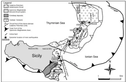
The Sicily island, in south of Italy, is one of the Mediterranean area characterised by high seismic risk. Figure 1.14 shows Sicily and the main active faults that influence the seismicity of this area. The collision between the two continental plates (African and European) is the source of the seismic activity along the fault that goes though Sicily and Ionian Sea.

Figure 1.14 Tectonic framework of the study area with major structural domains of southern Italy and active faults identified through surface

geological evidence

Eastern Sicily is delineated by the crossing of lithosphere structures that give rise to the origin of Mt. Etna and by the presence of the Malta Hyblean fault system that goes down to the Sicilian coast towards the Ionian Sea. The definition of seismic sources in eastern Sicily is a quite debated problem due to the lack of clear evidence of surface faulting and to the few high-magnitude instrumental earthquakes. For example, the location, size and kinematics of the January 11, 1693 earthquake (MW= 7.4, [2]) is particularly uncertain and debated in literature. Some authors locate the source inland, whereas others locate it offshore. The inland source models are based on geologic, geomorphologic and macro seismic intensity analyses. On the other hand, the models that adopt an offshore source are mainly based on results of seismic prospecting at sea

(37)

and on tsunami modelling which suggests either the rupture of a segment of the NNW-SSE Malta fault escarpment [3, 4, 5]; or the rupture of a locked subduction fault plane [6]. Recently, some authors associated the 1693 earthquake to the Sicilian basal thrust, to which they associated the 1818 Catania event (MW = 6.2, Working Group CPTI, 2004) as well [7]. In eastern Sicily, in addition to the seismicity related to these regional sized tectonic structures, there is an intense seismic activity due to the Etna volcano. It is characterized by low magnitude events and shallow hypocentres that produce destructive effects only at local scale [8].

Figure 1.15 Tectonic sketch and Epicentral map of the regional earthquakes.

1.4 _{Historical seismic events in Catania}

The seismic activity in the Catania area is particularly high, as testified by the historical earthquakes. The main earthquakes that hit Catania occurred in 1169, 1542, 1693 and 1818 while the more recent, although moderate, occurred in 1990.

The main Catania urban changes have been determined by natural catastrophes such as volcano eruptions and massive earthquakes. Historical Etnean lava flows invaded and partially covered the ancient city of Catania many times (e.g., 683 BC, 252 AC) and several seismic events stroke the city in the millennia.

(38)

16

Basing on several researches on the Catania seismic history [9, 10, 11, 12], a short overview is proposed below.

4th_{February 1169}

On the 4th February 1169, a heavy earthquake stroke the Sicily at 7:00 am on the eve of the feast of St. Agatha of Sicily. It had an estimated magnitude between 6.4 and 7.3 and an estimated maximum perceived intensity of X (Extreme) on the Mercalli intensity scale [9]. Catania was deeply damaged. The earthquake triggered a tsunami as well. Overall, 15,000 people died during the earthquake and they were almost the 65% of the entire population [9].

10th_{December 1542}

This event caused several damages in the Ionian coast, but the seismic waves were felt through the whole island. The main shock was followed by a seismic period that started die ultimo mesis novembris (the last day of November) and continued for 40 days. Catania was severely damaged. Churches, monasteries and buildings completely or partially collapsed. Many structures were severely hit. A whole quarter in the western part of the city ruined.

8th_{March 1669}

In the 1669, a devastating Etna eruption changed the town planning. The lava flowed in the western sector of the ancient town, destroyed part of it and its volume was able to fill up the moat of Ursino Castle.

(39)

9 and 11 January 1693

This was the most destructive event that the Italian country knew [13]. The 1693 Sicily earthquake struck parts of southern Italy near Sicily, Calabria and Malta on January 11th at around 9 pm local time. This earthquake was preceded by a damaging foreshock on January 9th. The main shock had an estimated magnitude of 7.4 on the moment magnitude scale, the most powerful in Italian history, and a maximum intensity of XI (Extreme) on the Mercalli intensity scale, destroying at least 70 towns and cities, seriously affecting an area of 5,600 square kilometres and causing the death of about 60,000 people. A tsunami happened and it destroyed several villages by the sea on the Ionian Sea and in the Straits of Messina. Almost two thirds of the entire population of Catania died (between 12 and 16 thousand victims over a population of 18-20 thousand people). The rebuilding process converged in a new and homogeneous Baroque style. The towns and villages of southeastern Sicily, particularly in the Val di Noto, were rebuilt in this new and elegant architectural style, described as "the culmination and final flowering of Baroque art in Europe". [13]

The old urban planning was replaced by a newest characterized by larger main roads cut off of squares, with a kind of anti-seismic aim.

(40)

18

20th_{February 1818}

The earthquake damaged several buildings in Catania did not caused victims. The buildings had internal collapses and widespread damages.

11th_{January 1848}

The earthquake of the 1848 was the last serious seismic event that struck Catania. Nobody died in that event and there were few minor collapses of ornamental stones of façade parts.

The city of Catania grew hugely in the 19th_{century. At the end of the}

20th_{century, between the 1960s and 70s, Catania, and Italy in general,}

knew its maximum urban expansion. This was the decade of the huge residential blocks, according to the contemporary architectural and urban philosophies.

Catania landscape started to be marked by mid-rise buildings, designed only for gravity loads and founded on rocks or soft soils as in some areas over the rubble of the 1963 earthquake that are generally characterised by an amplification of the seismic signals.

1.5 _{Definition of the seismic inputs}

Aiming at performing seismic assessment of the different structural models under investigation by means of nonlinear dynamic analyses, the selection of suitable seismic inputs (accelerograms) is required. These could be obtained by considering the outcomes of numerous research works already performed for the Catania area or the oriental Sicily [14] or through a further seismological survey. However, the need to provide code-consistent seismic assessments as well as to investigate seismic retrofitting solutions to be applied in current practice led the choice towards the definition of simulated accelerograms compatible with the current design spectrum.

The literature divides the accelerograms in three main groups [15]. The first type consist of artificial spectrum-compatible accelerograms. Usually, they are obtained by procedures that generate power spectra density function from the smoothed response spectrum, and sinusoidal signals are then derived having random phase angles and amplitudes. The sinusoidal motions are then summed, and an iterative procedure can

(41)

be invoked to improve the match with the target response spectrum, by calculating the ratio between the target and actual response ordinates at selected frequencies. The power spectral density function is then adjusted by the square of this ratio and a new motion is generated. The second type consists of synthetic accelerograms generated from seismological source models and accounting for path and site effects. Finally, the third type involves the use of real recorded accelerograms. This last strategy is becoming more promising due to the increasing number of real records available by means of web-facilities and software [16] and web-databanks [17, 18, 19, 20, 21], making the use of real accelerograms a relatively straightforward and effective task [22].

Currently, the Italian national code and the European code allow defining seismic accelerations based on a spectral shape-based match. The artificial or adjusted inputs are individually compared to the elastic design spectrum, while the real recorded accelerograms are compared in terms of average values. In the latter respect, the Italian Seismic Code [23, 24] allows the use of real accelerograms, and imposes that these have to be compatible with the target spectrum in a specific range of vibration periods. Furthermore, the Italian Seismic Code states that the spectrum compatibility has to be achieved by the average real spectrum with the  =5% damping elastic response spectrum in the interval of 0.15s-2s and no less than the variance of 10% (Figure 1.18).

(42)

20

In this research, a set of seven accelerograms, in their three components, has been used and the match with the target spectrum has been achieved by means of a linear scaling iterative procedure. The choice is consistent to the Italian Code and Eurocode prescriptions that allow considering the mean structural response from the nonlinear dynamic analysis if at least seven sets of accelerograms are selected.

The accelerograms have been defined by means of the software REXEL v3.5 [16]. It automatically provides the identification of the recorded accelerograms and verifies the spectrum compatibility. All the three components for each accelerograms have been considered, and the spectrum compatibility has been satisfied for the planar and vertical target spectrum.

Looking at the definition of the seven accelerograms, the disaggregation of the seismic hazard has been performed. This procedure allows identifying the parameters that influence the seismic hazard of a specific site. By means of the disaggregation, the modal values of Magnitude (M) and epicentral distance (R) can be defined. Their combination defines the probability of exceedance a related PGA in the defined return time (Tr).

Specifying the M and R intervals equal to 6-7 and 10-30 km, respectively, assigning a compatibility tolerance with respect to the average spectrum of 10% lower and 30% upper in the period range 0.15– 2 sec the software returns the combinations of accelerograms shown in Figure 1.20 and Figure 1.21.

The target spectrum is defined by the values in Table 1-1.

Table 1-1 Target Spectrum

Lon. [°]: Lat. [°]: Site class: Top. cat.: Vn: CU: SL: 15.105 37.516 D T1 50 years II SLC

(43)

Figure 1.19 (Colour) Disaggregation in terms of Magnitude and Epicentral Distance for a Return Time of 475 year related to a Vt of 50 years and a soil

type D (SLC. Soil D. Category T1)

Table 1-2 Main characteristics of the seven adopted records

Waveform ID Earthquake ID Station ID Earthquake Name Date Mw Fault Mechanism Epicentral Distance [km] EC8 Site class 343 142 SMTC Christchurch 2011_February_21 6.2 reverse 16.52 C* 388 149 PPHS Christchurch 2011_June_13 6 reverse 13.44 C* 421 46 CLT Irpinia 1980_November_23 6.9 normal 18.85 B 391 149 SMTC Christchurch 2011_June_13 6 reverse 14.86 C* 340 142 PPHS Christchurch 2011_February_21 6.2 reverse 14.38 C* 444 89 EMO Imperial Valley 1979_October_15 6.5 strike-slip 19.33 C 431 77 AI_137_DIN Dinar 1995_October_01 6.4 normal 0.47 C

mean: 6,314 13,97857143

Waveform ID PGA_X [m/s^2] PGA_Y [m/s^2] PGV_X [m/s] PGV_Y [m/s] ID_X ID_Y Np_X Np_Y 343 17.791 13.823 0.32596 0.22313 44.116 84.186 0.82095 0.88607 388 13.114 12.408 0.16771 0.18485 91.643 10.614 10.666 0.90819 421 17.177 1.55 0.29058 0.26018 170.711 164.311 0.91751 0.74678 391 0.8071 0.91367 0.10986 0.15112 116.701 87.824 11.438 0.79114 340 20.909 19.239 0.36407 0.46143 78.201 63.566 0.97392 0.98503 444 2.904 30.761 0.90421 0.71742 25.661 24.267 0.83861 11.843 431 32.125 27.292 0.44387 0.29856 89.025 126.863 0.81449 0.95534 mean: 1,974672144 1,830847524 0,372324283 0,328098736 8,800817951 9,387963884 0,939417673 0,922402656

(44)

22

Figure 1.20 (Colour) Planar spectrum compatibility

Figure 1.21 (Colour) Vertical spectrum compatibility

Finally, the accelerograms have been handled and their duration has been uniformly set to 25 seconds aiming to obtain a similar computational time effort. The length of each accelerograms has been reduced and an exponential decay has been applied on the last 8 seconds. Lastly, the spectrum compatibility has been checked again. The process has been handled through an iterative procedure through a numerical routine. In Figure 1.22 a flowchart of the adopted strategy for the

(45)

accelerograms identification is reported. Figure 1.23 shows the spectrum compatibility of the obtained accelerograms in terms of planar and vertical components. Finally, Figure 1.23 depicts the three components of the obtained accelerograms.

Figure 1.22 (Colour) Flowchart of the procedure for defining the accelerograms

(46)

(47)

(48)

(49)

CHAPTER 2. I

NTRODUCTION TO THE

PROGRESSIVE COLLAPSE

AND ROBUSTNESS

ASSESSMENT

he present Chapter introduces the Progressive Collapse and the concept of Robustness with reference to multi-storey buildings. The Section aims to describe progressive collapse mechanisms due to typical damage scenarios in frame structures. According to different approaches, the assessment of a structure in a column loss scenario is discussed and different methodologies are described and commented. Since a unique assessment procedure does not exist, the overload factor [25] and the

simplified dynamic assessment [26, 27] are assumed as representative of

three different assessment strategies. Since simplified dynamic

assessment, developed by professor B.A. Izzuddin at the Imperial

College of London, has been adopted in the subsequent investigations it is accurately described.

(50)

(51)

2.1 _{Introduction to Progressive Collapse and}

Robusteness

The last decades have seen significant growth of scientific interest on the response of structures subjected to local damage eventually leading to progressive collapse (Figure 2.1). The attention was influenced by numerous partial or global structural failures occurred in the recent past and trigged by accidents or malicious acts. Some of the results obtained in previous studies have been incorporated in current standards [28, 29, 30, 31] providing specific robustness design prescriptions for new buildings.

Figure 2.1 Growth of number of publications between 1964 and 2016 (scopus.com)

Thus far, not all the design codes incorporate specific prescription in order to assess the influence of local damage on the global behaviour of the overall structure with the aim to avoid that a local damage can lead to a disproportional collapse. So far, a unique and shared definition of the progressive collapse nomenclature has not been still produced. Due to this reason, two main concepts that define the phenomena and the structural attitude of withstanding local collapses have slightly different definitions. Storessek [32] attempted to coin a satisfactory definitions for

Collapse Resistance and Structural Robustness, covering the several

definitions that he found in codes and researches. He defined: 0 50 100 150 200 250 19 64 19 65 19 66 19 67 19 68 19 69 19 70 19 71 19 72 19 73 19 74 19 75 19 76 19 77 19 78 19 79 19 80 19 81 19 82 19 83 19 84 19 85 19 86 19 87 19 88 19 89 19 90 19 91 19 92 19 93 19 94 19 95 19 96 19 97 19 98 19 99 20 00 20 01 20 02 20 03 20 04 20 05 20 06 20 07 20 08 20 09 20 10 20 11 20 12 20 13 20 14 20 15 20 16 N u m be r of p u bl ic at io n s Years Progressive collapse

(52)

30

Collapse Resistance the structural insensitivity to accidental (and

rare) circumstances (extreme loading events), which are low probability events and unforeseeable incidents.

Structural Robustness the insensitivity to local failure, where

“insensitivity” and “local failure” are to be quantified by the design objectives that are parts of the design criteria.

2.1.1_{Design strategies against progressive}

collapse

The design codes adopted specific design strategies for new buildings to withstand disproportional collapses due to local failures. The design prescription are generally defined as Bridging, Tie and Segmentation

Method.

The Bridging Method, usually called Alternative Load Path [33], aims to describe the structure in the damaged configuration. In new structures, the absence of bearing elements returns an alternative structural scheme in which the other elements have to be able to withstand forces redistribution. The capacity to resist global collapse in case of heavy local damages has to be verified in new structures according to several design codes [30, 31, 29].

The Tie Method is an indirect design method based on the capacity of prescribed structural elements to redistribute the forces during the collapse and contain its extension to the entire building. Figure 2.2 shows a scheme of this method. The ultimate version of the “Alternate Path Analysis & Design Guideline for Progressive Collapse Resistance” (GSA) [33] exclude the tie strategy even though it is still present in the “Design of Buildings to Resist Progressive Collapse” Unified Facilities Criteria (DOD-UFC) [31].

(53)

Figure 2.2 Tie Forces in a Frame Structure

Lastly, Segmentation is an alternative design strategy. The presence of weak elements within the structures can arrest the propagation of the collapse. It can be explicitly adopted in the design process or intrinsically present in existing structure designed under gravity loads only for instance. The absence of seismic detailing does not guarantee the continuity of reinforcement steel bars. On one hand this type of structures do not have resource to resist local collapses, on the other hand, the reinforcement local discontinuities can arrest disproportional collapses, causing partial collapse of the structure.

(54)

32

2.2 _{Review of prominent progressive collapses}

As the Figure 2.1 shows, the last two decades saw the growing of interests on progressive collapse. Few strategic or relevant buildings suffered of progressive collapse, trigged by accidental or malicious events in the modern era. However, some of these events started the research interest in progressive collapse with the aim to identify the mechanisms that the structural elements develop during a local collapse and identify strengthening solution and appropriate design approaches. Few famous very important progressive collapse events had a flywheel effect on the scientific research that was also supported by governments. In 1968, the Ronan Point Tower, placed in Canning Town near London, England, went through a disproportional collapse (Figure 2.3) due to an accidental gas explosion [34]. The building was a 22-storey residential block made by precast panels joined each one other without framed structure. The accidental event, trigged by a gas blast at the 18th

floor at the southern corner, caused the collapse of the superior levels due to the leak of connection between the panels and the floor slabs. The construction technology defined the collapse of the floors but, at the same time, avoided the collapse propagation thanks to the segmentation that had a key role in the collapse mechanism. After this tragedy, the United Kingdom design code made mandatory structural details and design process to avoid disproportional collapse [35] in the new designed buildings.

Seismic Assessment and Rehabilitation of existing RC Buildings not designed to withstand earthquakes

Buildings not designed to

withstand earthquakes

Giuseppe Occhipinti

Declaration

Abstract

vi

Acknowledgments

Table of Contents

xii

List of Tables

List of Figures

xviii

xx

xxii

CHAPTER 1.

C

ATANIA

’

S

S

EISMIC

H

AZARD

1.1

Background

4

6

1.2

Seismic Hazard in Italy and Seismic Code

evolution

8

10

12

14

1.3

Seismic Hazard in Sicily

1.4

Historical seismic events in Catania

16

18

1.5

Definition of the seismic inputs

20

22

CHAPTER 2.

I

NTRODUCTION TO THE

PROGRESSIVE COLLAPSE

AND ROBUSTNESS

ASSESSMENT

2.1

Introduction to Progressive Collapse and

Robusteness

30

32

2.2

Review of prominent progressive collapses

_Background

_{Seismic Hazard in Italy and Seismic Code}

_{Seismic Hazard in Sicily}

_{Historical seismic events in Catania}

_{Definition of the seismic inputs}

_{Introduction to Progressive Collapse and}

_{Review of prominent progressive collapses}