When probabilistic seismic hazard climbs volcanoes: the Mt. Etna case, Italy – Part 2: Computational implementation and first results

© Author(s) 2017. This work is distributed under the Creative Commons Attribution 3.0 License.

When probabilistic seismic hazard climbs volcanoes: the Mt. Etna

case, Italy – Part 2: Computational implementation and first results

Bruno Pace4_{, Marco Pagani}5_{, Francesco Panzera}3_{, Mario Ordaz}6_{, Miguel Leonardo Suarez}6_{, and Giuseppina Tusa}2 1_{Istituto Nazionale di Oceanografia e di Geofisica Sperimentale – OGS, 34010 Sgonico (TS), Italy}

2_{Istituto Nazionale di Geofisica e Vulcanologia (INGV), 95123 Sezione di Catania – Osservatorio Etneo, Italy} 3_{Dept. of Biological, Geological and Environmental Science, University of Catania, 95129 Catania, Italy} 4_{DiSPUTer, University “G. d’Annunzio” Chieti-Pescara, 66013 Chieti, Italy}

5_{GEM Foundation, 27100 Pavia, Italy} 6_{UNAM, 04510 Coyoacan, CDMX, Mexico}

Correspondence to: Laura Peruzza (lperuzza@inogs.it) Received: 30 March 2017 – Discussion started: 5 April 2017

Revised: 20 September 2017 – Accepted: 24 September 2017 – Published: 22 November 2017

Abstract. This paper describes the model implementation and presents results of a probabilistic seismic hazard assess-ment (PSHA) for the Mt. Etna volcanic region in Sicily, Italy, considering local volcano-tectonic earthquakes. Working in a volcanic region presents new challenges not typically faced in standard PSHA, which are broadly due to the nature of the local volcano-tectonic earthquakes, the cone shape of the volcano and the attenuation properties of seismic waves in the volcanic region. These have been accounted for through the development of a seismic source model that integrates data from different disciplines (historical and instrumental earthquake datasets, tectonic data, etc.; presented in Part 1, by Azzaro et al., 2017) and through the development and software implementation of original tools for the computa-tion, such as a new ground-motion prediction equation and magnitude–scaling relationship specifically derived for this volcanic area, and the capability to account for the surfi-cial topography in the hazard calculation, which influences source-to-site distances. Hazard calculations have been car-ried out after updating the most recent releases of two widely used PSHA software packages (CRISIS, as in Ordaz et al., 2013; the OpenQuake engine, as in Pagani et al., 2014). Re-sults are computed for short- to mid-term exposure times (10% probability of exceedance in 5 and 30 years, Poisson and time dependent) and spectral amplitudes of engineer-ing interest. A preliminary exploration of the impact of site-specific response is also presented for the densely inhabited

Etna’s eastern flank, and the change in expected ground mo-tion is finally commented on. These results do not account for M > 6 regional seismogenic sources which control the hazard at long return periods. However, by focusing on the impact of M < 6 local volcano-tectonic earthquakes, which dominate the hazard at the short- to mid-term exposure times considered in this study, we present a different viewpoint that, in our opinion, is relevant for retrofitting the existing buildings and for driving impending interventions of risk re-duction.

1 Introduction

It is well known that volcanoes and earthquakes are associ-ated everywhere, although volcanic seismicity is extremely diversified and is associated with a variety of volcanic pro-cesses (Zobin, 2012). In some active volcanic zones, namely the most populated ones, these earthquakes may cause se-vere damage to buildings and lifelines, representing a fur-ther source of hazard in addition to the ones posed by the eruptive activity (e.g., Zobin, 2001). Some major worldwide examples of M6–M7 earthquakes in different volcanic envi-ronments are from Japan, Indonesia, Hawaii and the Azores islands (Abe, 1979; Yokoyama, 2001), whilst in mainland Europe the Mt. Etna volcano represents a case where low-magnitude events produce local effects of high intensity

(Az-zaro, 2004; Azzaro et al., 2013). Since seismic hazard is as-sociated with expected earthquakes, why can we not usu-ally pinpoint volcanoes on a hazard map? In general, the effects of volcanic earthquakes can be overshadowed by the stronger tectonic regional earthquakes, particularly when long exposure periods are considered. Furthermore, due to their low magnitudes and the high attenuation typically ex-hibited in volcanic regions, most ground-motion prediction equations (GMPE) are not applicable for such events. We faced these challenges, among others, in the seismic haz-ard study of Mt. Etna, one of the most active volcanoes in a long-lasting inhabited area in the Mediterranean. In a few kilometers it is possible to walk from the ancient Greek and Roman archaeological remains of the coast to hostile and de-serted summit craters 3.3 km above sea level (a.s.l.). While catastrophic earthquakes and tsunamis occur in eastern Sicily on average every 3–4 centuries (Azzaro et al., 1999), build-ing collapse, casualties and road interruptions due to shallow, light-to-moderate earthquakes (M4–M5) happen much more frequently on the flanks of Mt. Etna (e.g., D’Amico et al., 2016). These earthquakes are linked to surficial fault sources that breathe with the tectonic stresses and the volcanic dy-namics.

In recent years, several analyses have been undertaken to estimate the short- to mid-term (5–30 years) capability of local faults on Mt. Etna to generate damaging or destruc-tive earthquakes. Two main approaches have been explored. The first is a probabilistic seismic hazard assessment (PSHA) based on macroseismic data, which uses a historical prob-abilistic approach (the “site-intensity approach”; see Az-zaro et al., 2008, 2016) to determine the localities prone to high seismic hazard at the local scale. The second is a seis-motectonic approach, where historical inter-event times of fault ruptures are investigated and used to generate an earth-quake rupture forecast (Azzaro et al., 2012, 2013). In this approach, both Poissonian occurrence probabilities of ma-jor earthquakes and time-dependent occurrence probabilities using a renewal processes that takes into account the time elapsed since the last event have been determined. Both ap-proaches have found that the local faults significantly con-tribute to the seismic hazard at Mt. Etna with respect to the larger tectonic structures, when short investigation times are considered.

In 2012 a new project started, namely the DPC-INGV V3 project (Azzaro and De Rosa, 2016), with one of its tar-gets being a new PSHA for the Etna region due to local volcano-tectonic earthquakes. Working in the Mt. Etna re-gion presents new challenges not usually faced in standard PSHA. These are due to (i) the nature of the local volcano-tectonic earthquakes, which are low-magnitude (partially out of the applicability range of most GMPEs) and have large ruptures compared to those predicted by commonly used magnitude scaling relationships (MSR); (ii) the cone shape of the volcano, where events are located within the vol-canic edifice above the sea level and therefore the

topogra-phy (elevation) of Mt. Etna must be considered, which in turn affects source-to-site distances in the hazard computa-tion; (iii) the attenuation properties of seismic waves in the Mt. Etna region, where shaking exhibits a rapid attenuation particularly at high frequencies; and finally (iv) the hetero-geneities in rock properties within the volcanic body, so that proxies simply based on slope or surface geological mapping are not adequate to represent reliable site-specific effects. To address these challenges, we used two PSHA software pack-ages (CRISIS, as in Ordaz et al., 2013; the OpenQuake en-gine, as in Pagani et al., 2014) and developed new software functionalities to incorporate the topographic surface into the hazard calculation by modeling sources and sites above the sea level. We also derived new empirical relationships specif-ically for Mt. Etna, such as a MSR (described more in detail in the companion paper, Azzaro et al., 2017, hereinafter re-ferred to as Part 1), and a GMPE presented here. In this pa-per we summarize the source model, discuss the model im-plementation, new GMPE and software functionalities, and finally present the hazard results. We hope the results of this study may be integrated into a more traditional, national reg-ulation framework (e.g., Stucchi et al., 2011) with realistic and useful ground-motion prediction maps devoted to urban planners and structural designers.

2 Seismic source model: conceptual components The seismic source modeling at Mt. Etna accounts for three different levels of increasing complexity, and sources are modeled using distributed seismicity as well as faults. The source model accounts for some basic assumptions be-hind the physical processes driving earthquake occurrences, which in our volcanic area refer to the brittle failure of rocks under tectonic stress producing volcano-tectonic earth-quakes along well-known surface rupturing faults. In partic-ular: (i) the damaging earthquakes at Mt. Etna feature very shallow foci; (ii) these shocks, which are mainly concen-trated on the southeastern flank of Mt. Etna, occur with about decennial frequency (see, for example, Azzaro et al., 2012, 2013; Sicali et al., 2014) with or without synchronous vol-canic activities; (iii) the last major events and interseismic periods have been monitored by a dense, high-quality in-strumental local network whose geometry and characteris-tics have essentially remained unchanged during in the last 2 decades (Alparone et al., 2015).

For a full description of the individual model compo-nents and the process of defining seismic sources, we refer the reader to Part 1. Different seismic sources were defined for representing the shallow volcano-tectonic seismicity at Mt. Etna, after checking that a few years of high-quality seis-mic monitoring, during an interseisseis-mic period, can be rep-resentative of the long-term seismic rates of the volcano-tectonic faults; this simplification is supported by about 2 centuries of detailed field observations and chronicles,

de-Figure 1. Source typologies at Mt. Etna. (a) Polygonal area sources representing uniform seismicity: the ones defined in this study (in pale blue and yellow) follow the seismogenic sections of the best-known fault systems; in orange is the single area source used in the map of Italian regulation (ZS9, Stucchi et al., 2011).(b) Fault sources modeling the main volcano-tectonic structures detected on Etna’s flanks (see Table 1 for the nomenclature): the red boxes and lines represent the projection at the surface of the fault planes.(c) Three-dimensional mesh of point sources, used to model the scattered background seismicity, with b values represented by colors. Details are given in Part 1 (Azzaro et al., 2017).

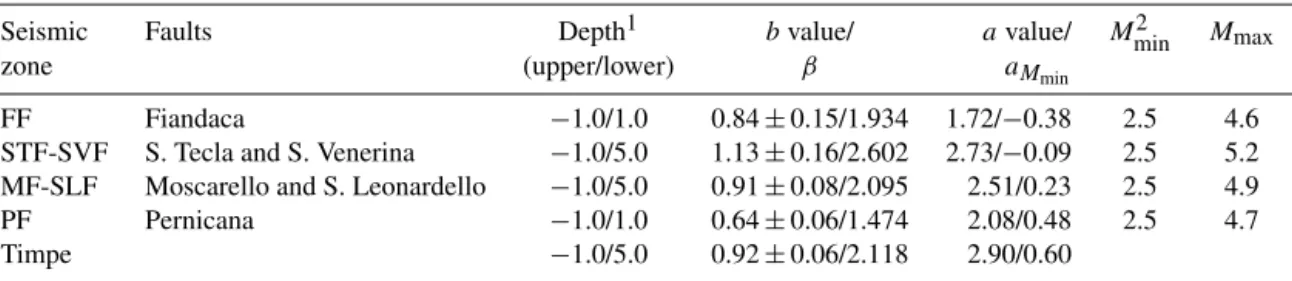
Table 1. Parameters of area seismic sources used in the final computations.

Seismic Faults Depth1 bvalue/ avalue/ M_min2 M_max

zone (upper/lower) aMmin

FF Fiandaca 1.0/1.0 0.84 ± 0.15/1.934 1.72/ 0.38 2.5 4.6 STF-SVF S. Tecla and S. Venerina 1.0/5.0 1.13 ± 0.16/2.602 2.73/ 0.09 2.5 5.2 MF-SLF Moscarello and S. Leonardello 1.0/5.0 0.91 ± 0.08/2.095 2.51/0.23 2.5 4.9 PF Pernicana 1.0/1.0 0.64 ± 0.06/1.474 2.08/0.48 2.5 4.7 Timpe 1.0/5.0 0.92 ± 0.06/2.118 2.90/0.60

1_{Negative depth means above the sea level.}2_{The ground motion out of the range 3.0 < Ml<4.3 is extrapolated.}

scribing the seismotectonic evidence, and by the more re-cent deformation rates derived from geodetic measurements. We accept this working hypothesis and thus parameterize seismic sources by extrapolating decennial datasets. We can also model by means of point sources faults that are still “unknown” as they are not recognized at the surface, and compute earthquake probabilities using any time/magnitude– frequency distribution (FMD), thus abandoning the require-ments of independence and stationarity of events needed by the Poisson process.

The seismic sources considered at Mt. Etna take into ac-count the huge amount of available geological, historical, seismological and geodetic data. The three types of seismic sources depicted in Part 1 are as follows (see Fig. 1 and con-cept scheme in Fig. 2):

– Area seismic sources (Fig. 1a) are zones of distributed (i.e., uniform) seismicity. These encompass the best-known fault systems on the Mt. Etna’s flanks. They are defined in both CRISIS and the OpenQuake engine by a horizontal planar surface, modeled as a series of point

sources with spatially extended ruptures. This approach is the same used by the current seismic hazard map of Italian regulation (MPS04, Stucchi et al., 2011), where the whole volcanic body is enveloped in a single polyg-onal area.

– Fault sources (Fig. 1b) model the main tectonic struc-tures. The geometries are based on surface ruptures and other geological and geophysical investigations. Faults are modeled in the OpenQuake engine by a mesh of points defined by top and bottom (and optionally mid-dle) edges, whose 3-D geometry may change in dip and width and extended ruptures float along strike. In CRI-SIS, faults are represented by planes of given coordinate vertexes.

– Point sources (Fig. 1c) are used to represent distributed (i.e., gridded, nonuniform) seismicity. The distributed seismicity is defined in the same way by CRISIS and the OpenQuake engine, using point sources with spatially

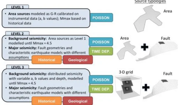
Figure 2. Schematic chart describing the three branching levels of the source model and depiction of the different source typologies used for modeling. The major seismicity of levels 2 and 3 is modeled using fault sources, where seismicity rates are derived using historical and geological approaches, considering both time independence (Poisson) and time dependence.

extended ruptures and variable properties (e.g., seismic-ity, depth).

In this case study, the sources extend above the sea level to model the earthquakes within the volcanic edifice, and also the faults intersect the topographic surface.

These sources are combined together to form alternative seismic source models. Three source model branching levels are defined, in order of increasing complexity, to represent the epistemic uncertainties (Fig. 2).

– Source Model Level 1 is composed of area sources only. Four zones of uniform seismicity are parameterized by Gutenberg–Richter (GR) FMDs calibrated on the best-quality instrumental catalogue (see Sect. 4.1 in Part 1) during an interseismic period that is considered repre-sentative of the long-term seismic behavior observed since the 19th century. Seismicity rates are extrapolated until the maximum magnitude observed in the historical period (Mmax= 5.2), and effective depths are estimated

by the analyses of strain release profiles. The values of parameters entered in both the OpenQuake engine and CRISIS are given in Table 1.

– Source Model Level 2 combines major earthquakes (M > 4.5) that are assigned to faults only, with back-ground seismicity that is assigned to area sources as in Level 1 (modeled up to Mmax= 4.5). The FMDs of

faults are Gaussian distributions peaked to the charac-teristic earthquake models; rates are branched, based on

the historical observations only, or constrained by ge-ometrical and geological–kinematic considerations on fault size and slip rate (observed and calculated mean recurrence time Tmeanand maximum magnitude Mmax

in Table 2; see Pace et al., 2016, for the method; Part 1 for results obtained at Mt. Etna). In Table 2 we sum-marize the input data and the results in terms of oc-currence probabilities of the characteristic earthquake, following a memory-less process (Poisson) or introduc-ing the time dependency of the last event by a Brownian passage time (BPT) model for both the branches (histor-ical and geolog(histor-ical–kinematic). Note that the Pernicana fault (PF) is always modeled as GR, not having histori-cal observations supporting the choice of a characteris-tic earthquake model.

– Source Model Level 3 again assigns the major seismic-ity to faults, as in Level 2, but background seismicseismic-ity is modeled by distributed seismicity using scattered point sources (in 3-D) with spatially variable GR rates up to Mmax= 4.5. Since the hypocenters locations

deter-mined by a 3-D velocity model take into account the nonuniform crustal properties beneath the volcanic edi-fice, we prefer this model as it is essentially data-driven and less affected by subjective choices about zonation; we acknowledge that the picture of fragile deformation depicted by the recent low-magnitude seismicity repre-sents the best available context currently.

Table 2. Parameters of fault sources used in the final computations. Historical: Mobs is the maximum observ ed magnitude; Tela is the elapsed time from the last maximum earthquak e; Tmean is the mean recurrence time of a maximum earthquak e; ↵ is the aperiodicity factor; probabilities are probabilities of a maximum magnitude, Poisson in 5 years (Pois), time dependent in the ne xt 5 (BPT 5 years) and 30 years (BPT 30 years) from 2015. Geological–kinematic: Mmax is the maximum expected magnitude; Mmax is the standard de viation of the maximum expected magnitude; Tmean is the mean recurrence time of maximum earthquak e; the other columns are as in historical. Fault Historical Geological–kinematic Mobs Tela Tmean ↵ Probabilities Mmax Mmax Tmean ↵ Probabilities Pois BPT BPT Pois BPT BPT 5 years 30 years 5 years 30 years Pernicana (PF) 4.7 15 71 0.42 5.4 ⇥ 10 2 1.2 ⇥ 10 4 8.0 ⇥ 10 2 5.0 0.4 28 1.39 1.2 ⇥ 10 1 1.7 ⇥ 10 1 5.9 ⇥ 10 1 Fiandaca (FF) 4.6 123 71 0.42 5.4 ⇥ 10 2 1.4 ⇥ 10 1 6.1 ⇥ 10 1 4.9 0.4 166 1.38 2.2 ⇥ 10 1 2.9 ⇥ 10 2 1.5 ⇥ 10 1 S. Tecla (STF) 5.2 103 71 0.42 5.4 ⇥ 10 2 1.3 ⇥ 10 1 5.9 ⇥ 10 1 5.3 0.4 53 1.41 6.6 ⇥ 10 2 5.5 ⇥ 10 2 2.7 ⇥ 10 1 S. V enerina (SVF) 4.6 15 71 0.42 5.4 ⇥ 10 2 7.5 ⇥ 10 5 6.6 ⇥ 10 2 5.0 0.4 45 1.40 7.8 ⇥ 10 2 1.3 ⇥ 10 1 5.0 ⇥ 10 1 Moscarello (MF) 4.9 106 71 0.42 5.4 ⇥ 10 2 1.3 ⇥ 10 1 5.9 ⇥ 10 1 5.5 0.5 119 1.76 2.6 ⇥ 10 2 3.2 ⇥ 10 2 1.7 ⇥ 10 1 3 GMPE at Mt. Etna

A key component of any seismic hazard assessment is the propagation of seismic energy from the source to the receiver, accounted for in a heuristic way by GMPEs, as the details of seismic wave propagation are usually unknown. Volcanic ar-eas often exhibit peculiar characteristics expressed by high attenuation of seismic energy, especially for shallow earth-quakes.

Concerning the geological conditions, the Mt. Etna vol-canic edifice overlies a thick sedimentary substratum with strong lateral heterogeneities (see, e.g., Branca et al., 2011; De Gori and Chiarabba, 2005). The foci of the shallow events (focal depth less than 5 km) fall into a depth range of the abovementioned sedimentary substratum; this affects both the seismic scaling laws (relationship of released seismic en-ergy and size of the source) and the wave propagation phe-nomena (Patanè et al., 1994; Giampiccolo et al., 2007; see Langer et al., 2016, for a more detailed discussion). Differ-ences between shallow and deep events (focal depth greater than 5 km) at Mt. Etna can be clearly identified just look-ing at the waveforms. For similar magnitude and distance, the shallow events have more low-frequency content than the deeper ones, where conversely the high frequencies prevail (Tusa and Langer, 2016). The distinctiveness of the shallow events makes the application of common ground-motion pre-diction equations used for tectonic areas questionable and in-appropriate.

For the purposes of DPC-INGV V3 project, we derived a local GMPE for the Mt. Etna region, focusing on the shallow events and using the high-quality data collected by the nu-merous seismic broadband stations that have been operating in eastern Sicily since 2006. We referred to the same sam-ple of data as Tusa and Langer (2016, hereafter TL16), the original GMPE developed for this project, but this time we considered a different distance metric (hypocentral distance instead of epicentral distance as required to incorporate to-pography into the calculation; see Sect. 4). The dataset con-sists of a set of 1200 three-component recordings acquired during 38 events in the magnitude range 3.0  ML 4.3 with

hypocentral distances between 0.5 and 100 km. Moreover, 95 % of the hypocenters are shallower than 2.5 km (more than 85 % of events have focal depth error equal or less than 0.5 km). Note that for our study area, recent investigations suggest that MLmatches MWvalues quite well (Saraò et al.,

2016). For an extensive description of data processing and the statistical characteristics of the data set, for example, in terms of magnitude, number of data-recording site classes and distance–magnitude distributions, we direct the readers to TL16. In order to compare our data to those recorded in other regions of Italy (in particular the Italian equation by Bindi et al., 2011, hereinafter ITA10), our empirical GMPE follows the simplified version of the formulation proposed by Boore and Atkinson (2008):

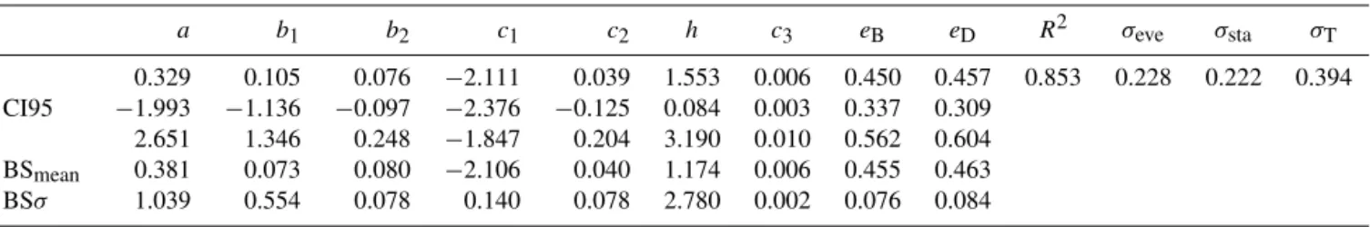
Table 3. Coefficients of Eq. (1) for the prediction of horizontal peak ground acceleration (gal) for the GMPE in this study. Magnitude is defined as ML. CI95 indicates the confidence intervals at 95 % confidence level. In this table, R2is the determination coefficient. eveand staare inter-event and inter-station terms of the errors, respectively. BSmeanand BS are the mean value and the standard deviation of each

coefficient, respectively, estimated by applying the bootstrap technique.

a b₁ b₂ c₁ c₂ h c₃ e_B e_D R2 _{eve sta T} 0.329 0.105 0.076 2.111 0.039 1.553 0.006 0.450 0.457 0.853 0.228 0.222 0.394 CI95 1.993 1.136 0.097 2.376 0.125 0.084 0.003 0.337 0.309 2.651 1.346 0.248 1.847 0.204 3.190 0.010 0.562 0.604 BSmean 0.381 0.073 0.080 2.106 0.040 1.174 0.006 0.455 0.463 BS 1.039 0.554 0.078 0.140 0.078 2.780 0.002 0.076 0.084 log(Y ) =a + b1M+ b₂M2+ [c₁+ c₂(M M_ref)] log⇣pR2+ h2/R_ref ⌘ + c3 ⇣p R2+ h2 R_ref ⌘ + eiSi+ T, (1)

where Mrefis a reference magnitude for magnitude

depen-dence of geometric spreading (here fixed to the mode value of the dataset, equal to 3.6), R is the hypocentral distance in kilometers, Rref is reference distance at which the near

source predictions are pegged (here fixed to a value of 1 km) and h is an additional parameter, referred to as “pseudo-depth”, incorporating all the factors that tend to limit or re-duce motion near the source (Joyner and Boore, 1981). The multiplier of the logarithmic distance term accounts for the magnitude-dependent ground-motion decay and controls the saturation of high-frequency ground motions at short dis-tances. Si indicates the soil conditions, with i standing for

the soil classes A–D defined in the EC8 building code. The Si variables of Boolean type are set to unity if the

corre-sponding soil class is met at a site, whereas the Sifor all other

classes is zero. Finally, Trepresents the total standard

devi-ation, which is the uncertainty in log(Y ) (logarithm is with base 10). The basic difference with TL16 is the distance met-ric, measured with respect to the hypocenter instead of the epicenter. This change allows accounting for the elevation of the seismic stations, which may vary in the range of about 2.5 km, a relevant difference, in particular for areas close to the epicenter.

The coefficients of our model, including the pseudo-depth h as well, were estimated applying the classical non-linear least-squares Marquardt–Levenberg algorithm as im-plemented in MATLAB. The coefficients of the model are computed by using an iterative least-squares estimation, with specified initial values. In particular, we tested different start-ing models in order to evaluate their effects on the solution, and at the same time, to select those values towards which the several inversions converged. The equations are derived from the regression analyses for horizontal peak ground ac-celeration (PGA) and 5 % damped spectral acac-celeration (SA) at several periods from 0.1 to 10 s. The regression coefficients and their 95% confidence intervals for PGAs are reported in

Table 3 (for SAs see the Supplement). The value of coeffi-cient c3, which stands for inelastic attenuation, is very close

to zero and could be potentially omitted from the functional form in Eq. (1). It has a minimal influence on the depen-dent variable values estimated through the obtained regres-sion model. The standard deviation obtained by bootstrap analysis is given too. The bootstrap bypasses problems in es-timating uncertainties of model parameters obtained in non-linear inversion, which is based on the Jacobian matrix and has the advantage of being applicable without a priori knowl-edge of the distribution of the underlying parent population. Compared to standard methods, the bootstrap yields a more robust and conservative estimation of parameter uncertain-ties. Here, in order to assess the stability of estimated regres-sion coefficients, we resampled our data set 1000 times and applied the same regression models as before. Each appli-cation gives a different set of regression coefficients and we calculate the statistics over our 1000 sets of coefficients.

The total standard deviation, T, can be split into two

terms:

T=

q

2

eve+ intraeve2 , (2)

where eveand intraeveare the intevent and intra-event

er-ror components, respectively, representing the erer-ror variabil-ity for different stations recording the same event and the er-ror variability for different earthquakes recorded by the same station. Similarly, if the variability among recording sites is taken into account, the total standard deviation of log(Y ) in Eq. (1) is given by

T=

q

2

sta+ intrasta2 , (3)

where sta and intrasta represent the inter-station and

intra-station component of the variance. We estimated the inter-group (inter-event and inter-station) and the intra-inter-group (intra-event and intra-station) variance – understood here in terms of mean square errors – for each attenuation model, by applying the “analysis of variance” test. We observe that the horizontal PGA has similar eve and stavalues, whilst the

spectral acceleration shows, in general, higher inter-station variability than the inter-event component, suggesting that

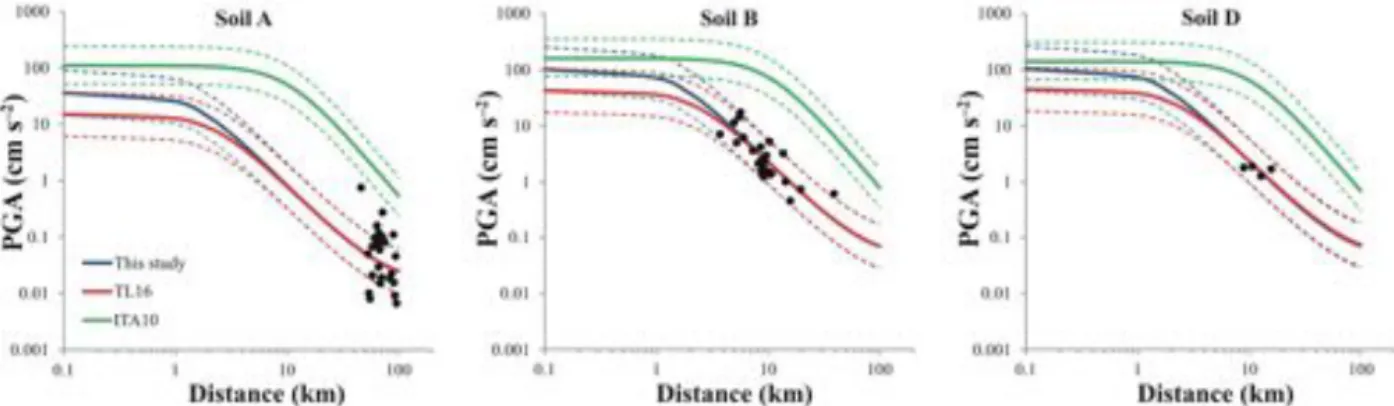
Figure 3. Predicted mean attenuation curves for a ML= 4 earthquake by the empirical law estimated in this study: ETNAhy, (continuous

blue lines), TL16 (continuous red lines) and ITA10 (continuous green line). The dashed lines represent the standard deviation of the mean. The black circles refer to the observations of our dataset with 3.9  ML 4.1; the three frames represent different soil types according to the

EC8 Building code.

the local site effects are the main source of ground-motion variability for our data.

In Fig. 3 we compare the predictions of horizontal PGA obtained in this study (coefficients reported in Table 3) with those derived by TL16 for shallow seismic activ-ity at Mt. Etna and by ITA10 for the whole Italian na-tional territory. Differences between the epicentral (TL16) and hypocentral versions of the GMPE (red and blue curves, respectively) are most evident for source-to-site dis-tances < 5 km, where the hypocentral version of the GMPE predicts higher accelerations. ITA10 (green curves) shows evident differences related to the flat part of the attenuation curves at short distances that goes from 0 to 10 km and more. The extension of this plateau depends critically on the h pa-rameter, and focal depths in ITA10 are larger than the one selected for Mt. Etna, thus leading to a higher h coefficient. Note that ITA10 is based on 793 records from 99 events and 150 stations, collected on the whole Italian territory; our data set offers at least the same or even a better statistical stabil-ity, from both the total number of records (1200) and cover-age (records per event, records per station and homogeneity from a seismotectonic point of view). From a practical point of view, the use of ITA10 strongly overestimates the PGA for shallow earthquakes at Mt. Etna as it predicts values which differ by a factor of about 3 near the source (distances < 2– 3 km) and much higher values (1–2 order of magnitude) at distances of 5–50 km. A quite different picture is obtained when spectral accelerations are taken into account, for ex-ample at T > 0.5 s, where ITA10 shows an underestimation of ground shaking (see Fig. S1 in the Supplement). This is due to the fact the spectra of shallow events at Mt. Etna are richer in low frequencies than the earthquakes normally con-sidered in GMPE, which are located at depth into the crys-talline basement.

The GMPE equations obtained by this study have been im-plemented in the software packages used for our analyses and will be referred to hereinafter as the ETNAhy GMPE model.

In CRISIS, the ETNAhy GMPE has been used by means of precompiled attenuation tables: an example for PGA and SA at 0.2, 0.4 and 1.0 s for soil type A is given as Supple-ment. Note that the magnitude range of applicability (stated in the data sample at 3.0–4.3 and slightly extended in this precompiled table up to values 2.6–5.3) covers values usu-ally not represented by standard GMPEs. In the OpenQuake engine, ETNAhy has been added to the library of GMPEs (https://github.com/gem), which also includes TL16, the ver-sion for Repi. Verification of the implementation was

per-formed by testing the expected mean and standard deviation output of the GMPE against a table of expected values pro-vided by the authors for different combinations of input vari-ables (e.g., magnitude, distance, Vs30).

4 Accounting for topography

Another implementation introduced in this study concerns the capability of taking into account the surface topography (elevation) in PSHA calculation. Typically in PSHA, the sites of the hazard computation are defined in terms of their ge-ographic coordinates on a planar surface representative of the sea level. This implies that the elevations of the sites are assumed to be zero, and the source-to-site distances in the PSHA calculation are computed accordingly. Usually this is an appropriate approximation because the actual elevations of the sites are small compared to the depths of the sources. However, in the case of Mt. Etna, this approximation cannot be made. Here, the earthquakes are shallow (mostly within the upper 5 km, and some even above the sea level inside the volcanic edifice) and the elevation of the volcano increases, sharply moving from the coast to the central craters, which are more than 3 km a.s.l.

A cross section of Mt. Etna is shown in Fig. 4, illustrating how the surface topography effects source-to-site distances. In this example, the distance Rhypo– as used by the GMPE

Figure 4. A topographic profile of Mt. Etna shown to scale, extending from the western side of the volcano to the eastern coast (Ionian Sea). Using a hypothetical fault, it can be demonstrated how the source-to-site distance increases (Rhypo2> R_hypo1) if the site is defined on the topographic surface (red triangle) compared to the sea level (clear triangle).

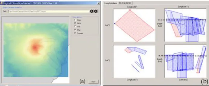
Figure 5. Snapshots of topography and sources in CRISIS. (a) DEM at Mt. Etna with area sources. (b) Preliminary release of fault sources in a 3-D view: the panel in the upper left shows a red fault plane which is projected with other fault sources in lower left; the panels on the right are classical cross sections along longitude (upper) and latitude (lower). Note the vertexes above the sea level, marked by black dashed lines in the cross sections.

in this study – increases when the topographic surface is in-cluded because the site elevation is increased. Note that for some source-to-site combinations, a straight path from the source to the site passes in the air above the free surface (for example if the site is at the very top of Mt. Etna and a shallow source is located a few kilometers away from the base) and therefore cannot be realistically followed by seismic waves. However, we find that the curvature of the topography is not pronounced enough (i.e., the slope of the topography changes gradually at the scale of the volcano) to cause a significant difference between a liner source-to-site path and a path that follows the free surface topography, and therefore we accept the approximation of a linear source-to-site path. Note that the influence of the topographic surface we describe here is purely a geometrical one and should not be confused with topographic site effects, where seismic waves are amplified in the vicinity of summits (see, for example, Imperatori and Mai, 2015, and references therein); improvements in rupture-to-site distance metrics related to topographic effects are be-yond the scope of this paper.

In order to correctly compute the source-to-site distances in the hazard calculation, we implemented the possibility to model a 3-D topographic surface into both software pack-ages. In CRISIS, this functionality has been added since the release V1.0 of 2015, by means of a specific layer that rep-resents the topography of the study area. A digital elevation model, given in a gridded data file, can be uploaded and the sites elevations are automatically computed on this surface (Fig. 5). The capability in the OpenQuake engine has been available since early 2017 (V2.3.0) and enables the user to specify the sites of the hazard calculation in terms of longi-tude, latitude and depth coordinates with respect to the sea level, for example in the form of a csv file. In both software packages, sources may also be defined above the sea level, using the convention of negative values for indicating eleva-tions above sea level.

This new functionality can be extended to other regions, although it is most appropriate in cases when the inclusion of topography is relevant to hazard (i.e., shallow sources with respect to the topographic elevation; see for example Peruzza et al., 2016), and source locations are well constrained with

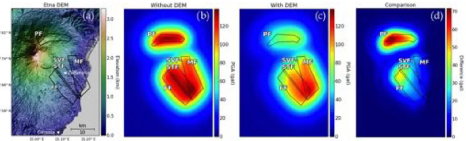
Figure 6. A hypothetical example showing the sensitivity of the hazard results to topography considering area sources and using the Open-Quake engine. The source geometries have assigned the same FMD and a depth of 2.5 km.(a) Etna DEM, (b) hazard without DEM (sites at sea level),(c) hazard with DEM (sites on topographic surface) and (d) residuals (given by b minus c values).

respect to the sea level, as is the case at Mt. Etna. In the-ory, site locations may also represent surfaces that are not exposed (e.g., the sea bottom, or bedrock lying below alluvial deposits), thus opening new potentialities for integrating site-specific response into hazard computation. As incremented capabilities may also introduce new problems for Mt. Etna analyses (i.e., how to account correctly for bedrock response if we are not in free-field conditions), we will accept the sim-plification that the topographic surface represents reference sites on bedrock.

We performed sensitivity tests at Mt. Etna to compare the software performances and to show the contribution of to-pography to the hazard. CRISIS and the OpenQuake engine behave the same in the simplest source formulation, e.g., area and point sources, and very similarly when complex faults are treated. To demonstrate the influence of topography, we use the same area sources as this hazard assessment but as-sign all of them the same FMD and a depth of 2.5 km, with the seismogenic layer extending from 0 to 5 km (Fig. 6). We find that including topography causes an increase in source-to-site distance and therefore a decrease in hazard that lo-cally reaches about 50 % of the values compared to the model that does not include topography. This effect is most pro-nounced in the regions of maximum elevation, notably the sources closest to the central craters (i.e., PF, the Pernicana area source). A similar effect is obtained by modeling fault sources too, but less pronounced as all the faults outcrop.

5 Accounting for site-specific response

We investigated the site-specific seismic response in the densely populated eastern flank of Mt. Etna by adopting the commonly used horizontal to vertical spectral ratio tech-niques that evaluate the site response properties using both earthquake (HVSR) and ambient noise (HVNR) as input sig-nals (Nogoshi and Igarashi, 1971; Nakamura, 1989; Lermo

and Chavez-Garcia, 1993). Although these methodologies are commonly applied in areas showing strong impedance contrast or minor lateral heterogeneities, they have been widely applied with valuable results in volcanic areas char-acterized by a complex geologic setting (e.g., Lombardo et al., 2006; Panzera et al., 2013, 2016, 2017; Rahpeyma et al., 2016).

The HVSRs were performed by selecting 30 local events that occurred in the volcanic area with ML>2.5; records were extracted from the INGV Osservatorio Etneo database, while location and magnitude were taken from the bulletins (Gruppo Analisi Dati Sismici, 2017). Recorded earthquakes were baseline corrected, with the purpose of removing spuri-ous offsets, and bandpass filtered in the range 0.08–20 Hz, with a fourth-order causal Butterworth filter. The analysis was performed by using 20 s time windows, starting from the S-wave onset, including part of the coda, and using a 5 % cosine-tapered window. Fourier spectra were smoothed us-ing a Konno–Ohmachi filter (Konno and Ohmachi, 1998) and the selected time window was compared with the pre-event noise in order to select good-quality data based on the signal-to-noise (S/N) ratio. For each recording, only those signals with S/N 3 were considered for analysis. The spectral ra-tios were evaluated at each station for the selected events and a geometric mean of all spectral ratios were computed to obtain the mean HVSR curve and the corresponding stan-dard deviation. The obtained HVSRs were grouped into four “spectral classes” by considering the frequency at which the dominant HVSR peak occurs, using the following criteria:

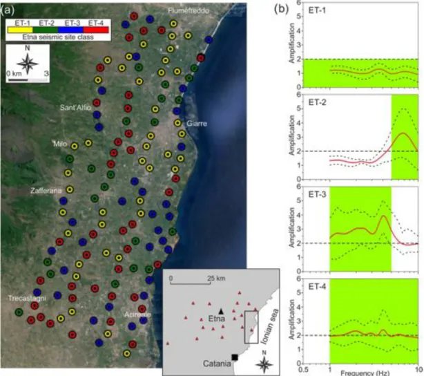
– ET-1 class: flat spectral ratios showing amplitude values not exceeding two units (including standard deviation); – ET-2 class: HVSR having fundamental period T  0.2 s

with amplitude exceeding two units;

– ET-3 class: HVSR with fundamental period 0.2 < T  1.0 s with amplitude exceeding two units;

Figure 7. Site amplification at Mt. Etna. (a) Sites investigated by HVNR measurements, where different colors point out the assigned “spectral class” given in the legend. In the inset map, location of the investigated area (black rectangle) and seismic stations (red triangles) used for the evaluation of the site amplification functions.(b) Site amplification functions (mean value in red, standard deviation with dashed black curves; see also Longo, 2017) obtained by grouping the HVSR inversions of seismic stations.

– ET-4 class: HVSR showing broadband amplitude ex-ceeding two units.

Besides, each experimental HVSR was inverted through ModelHVSR MATLAB routines (Herak, 2008) in order to compute theoretical HVSRs in homogeneous and isotropic layers. For the 19 considered seismic stations at Mt. Etna (stations locations are shown in the inset map of Fig. 7a), the stratigraphic sequence and local velocity model were made by integrating literature information and geological obser-vations (Azzaro et al., 2010; Branca et al., 2011; Branca and Ferrara, 2013; Panzera et al., 2011, 2015; Priolo, 1999). The soil models consist of a number of viscoelastic layers, stacked over a half-space, each of them being defined by the thickness (h), the velocity of the body waves (Vp and Vs),

the density (⇢) and the Q factor, which controls the inelastic properties. The code assumes that incoming waves are travel-ing vertically and considers that horizontal and vertical mo-tions at the bedrock have no amplification. The HVSR at the

surface is then obtained as the ratio between the theoretical transfer functions of S and P waves (Herak, 2008). The ob-tained HVSR output models were then used as input for the amplification function (AF) for 14 seismic stations. Five sta-tions, showing lack of convergence between the experimental and theoretical model, were removed. The AFs were com-puted through frequency-domain calculations, using the pro-gram SiteAmp by Boore (2003) that converts a velocity and density model into site amplifications. In particular, the For-tran code calculates the Thomson–Haskell plane SH-wave transfer function for horizontally stratified constant velocity layers at a specific incidence angle within a uniform velocity half-space. The input parameters are the Vs, the density (⇢)

and Q. The half-space is set at the deepest measured layer and the solution is exactly equivalent to the solution com-puted by the equivalent linear site response program SHAKE for linear modulus reduction and damping curves (Schnabel et al., 1972). The code computes the amplifications either at

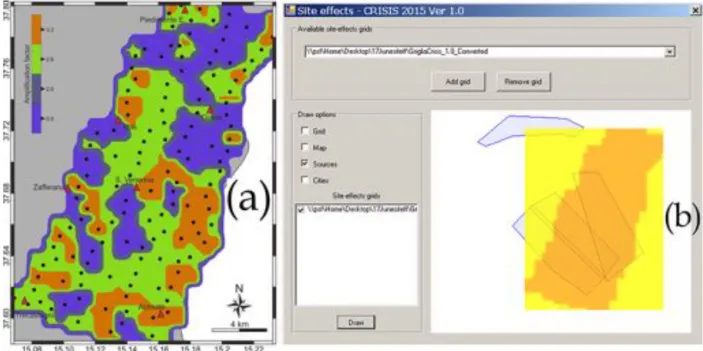
Figure 8. Simplified site-specific response along Mt. Etna’s southeastern flank. (a) Amplification factors at SA 0.2 s, obtained by interpolating the measured sites using the nearest neighbor algorithm.(b) Amplification factors as implemented in CRISIS; orange stripe represents the area where amplification factors enter in hazard computations.

specified frequencies or at frequencies corresponding to the “breakpoints” in the velocity model.

This procedure allowed us to assign an AF to each of the four HVSR classes previously identified by averaging the AFs of all the stations included in the class (Fig. 7b).

The European project Site Effects Assessment Using Am-bient Excitations (SESAME, 2004) found that the amAm-bient vibration method is a reliable alternative approach to using earthquake records especially for estimating the fundamental frequencies of a site. For this reason we performed a compar-ison between experimental HVSRs and HVNRs obtained at the seismic stations located around the volcano. The good matching obtained encouraged us to consider the ambient noise signal as a valid seismic input to be used to define the site fundamental frequency. We therefore proceeded to ob-tain the fundamental period classification in a wide sector of the lower eastern flank of Mt. Etna that includes 14 mu-nicipalities and many villages and rural settlements (Fig. 7a, colored dots). As highlighted in Part 1, this area is the most affected by strong shaking due to the seismogenic activity of the Timpe faults, and hence it is an appropriate choice for investigating the role of site-specific seismic responses. The fast and inexpensive HVNR technique has been performed by 130 georeferenced noise measurements recorded using a three-component velocimeter on a grid of sites quite ho-mogeneously spaced at about 1 km ⇥ 2 km distance. All the HVNRs in the present study were performed using time se-ries of 30 min length, with a sampling rate of 128 Hz. Sig-nals were processed by considering time windows of 30 s, selecting the most stationary part, excluding transients

asso-ciated with very close sources. In this way, the Fourier spec-tra were calculated in the frequency range of 0.1–30.0 Hz and smoothed using a proportional 20 % triangular window. Fol-lowing the criteria suggested by SESAME, only the spec-tral ratio peaks with amplitude greater than two units, in the frequency range 0.5–10 Hz, were considered significant. The obtained HVNRs were manually classified and grouped into the four classes of predominant period previously identified (colored dots in Fig. 7a).

A preliminary predominant-period site classification in the Mt. Etna’s eastern flank is finally attempted to overcome the one based on average shear wave velocity classification of the upper 30 m (Vs30). We mapped in the format required

by CRISIS the coefficients to be used in site-specific seis-mic hazard map, after interpolation of amplification factors at some spectral ordinates done by nearest neighbor algorithm (Fig. 8). According to Barani and Spallarossa (2016), this soil hazard method can be considered a hybrid probabilistic-deterministic method, and it may be useful to provide a first representation of seismic soil hazard at a large scale.

6 Results

We computed the hazard at Mt. Etna for the three source branching levels (depicted in Fig. 2), using the ETNAhy GMPE and the MSR derived specifically for this volcanic region as described in Sect. 3 and Part 1, respectively. Com-putations are for short-to-mid-exposure periods (10 % ex-ceedance probability in 5 and 30 years). Seismic hazard maps

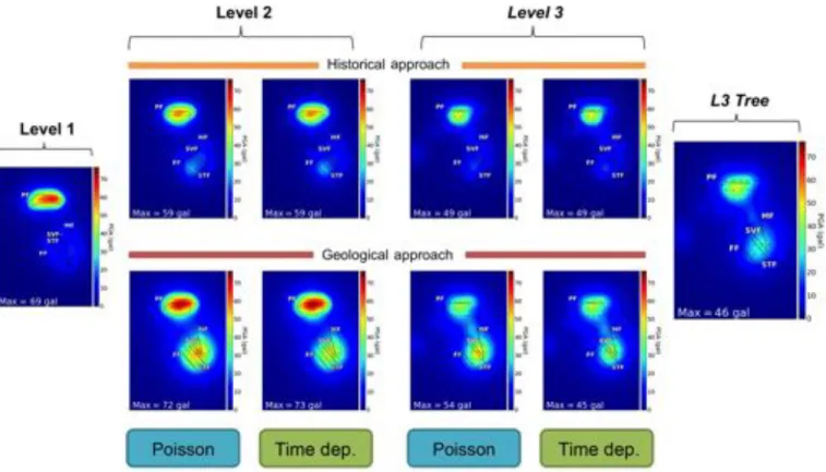
Figure 9. Hazard results for a 10 % exceedance probability in 5 years in terms of PGA, when Vs30= 800 m s 1. Thickest lines indicate fault

traces.

Figure 10. Hazard results for a 10 % exceedance probability in 30 years in terms of PGA, when Vs30= 800 m s 1. Thickest lines indicate

refer to rock conditions, where Vs30= 800 m s 1 (Figs. 9–

11), and exploratory site-specific results are also shown (Fig. 12).

The results obtained with the OpenQuake engine in terms of PGA are shown in Figs. 9 and 10. For a 5-year expo-sure period and a 10 % exceedance probability (Fig. 9), the maximum PGA (73 gal) is seen in Level 2, when using seis-mic rates calculated with the geological–kinematic param-eters under the time-dependent assumption (a BPT model is used, where the conditional probability of occurrence is based on the time elapsed since the last characteristic event; see Part 1 and Pace et al., 2016, for details). We find in gen-eral that the purely geological approach results in higher haz-ard compared to the ones obtained by the historical macro-seismic earthquake data (historical approach). For a 30-year exposure period (Fig. 10), the maximum PGA (274 gal) is seen in both levels 2 and 3, when using the geological– kinematic approach and Poisson model. Again, we observe that the geological–kinematic approach gives higher hazard compared to the historical approach (in this case, over 2 times higher), and that hazard is also higher when the occurrence rates on the faults have been derived using the Poisson model compared to the time-dependent model. Within the Timpe fault system, for both exposure periods, the Fiandaca fault (FF) dominates the hazard for the historical approach, while for the geological–kinematic approach the S. Tecla and S. Venerina faults (STF, SVF) dominate the hazard. To give context to these values, the current national hazard map (MPS04, see http://esse1-gis.mi.ingv.it/), which considers re-gional tectonic events not modeled in this analysis, shows PGA values around 0.20–0.25 g (196–245 gal) for the region of Mt. Etna, for an exposure period of 50 years. These val-ues fall between the historical and geological–kinematic ap-proaches of our analysis, considering an exposure period of 30 years. We performed a preliminary disaggregation test in terms of magnitude and distance considering only the area sources of Level 1 (time-independent model) and the four area sources from the MPS04 national hazard model closest to Mt. Etna; the results confirm that the hazard in our study area is dominated by the local volcano-tectonic events and not by the larger (M6+) events in the region for return times of 3–5 centuries.

We also used a logic tree in order to combine the results of the different models. The purpose of a logic tree is to account for the epistemic uncertainty, such as the three branching lev-els used here that represent different modeling approaches, meanwhile avoiding duplication of similar models. For this reason, we chose to neglect levels 1 and 2 in our logic tree weighting, under the assumption that the same information is contained in Level 3, i.e., the 3-D gridded seismicity is a more complex representation of the distributed seismicity in Level 1, and the fault sources are modeled in the same way as in Level 2. For the final logic tree, we therefore weighed the four models in Level 3 (historical Poisson, historical time dependant, geological Poisson, geological time dependant)

equally with weights of 0.25. In the final mean hazard maps, we obtained maximum PGA values of 46 and 176 gal, for exposure periods of 5 and 30 years, respectively. For a 5-year exposure period (Fig. 9, “L3 Tree” frame), the hazard is highest around the PF, while for a 30-year exposure period (Fig. 10, “L3 Tree” frame), the hazard is similarly high also around STF and SVF.

In some of the hazard maps, the hazard pattern appears concentrated around the middle of the fault sources in a ra-dial pattern. This is most notable around the PF using the geological–kinematic approach for an exposure period of 30 years. This is due to the combination of the following: (1) the fault sources have been assigned Gaussian FMDs centered near the magnitude of the characteristic earthquake (i.e., full fault rupture), and therefore finite ruptures which have areas defined by the Etna MSR (see Part 1) float min-imally along strike; and (2) the ETNAhy GMPE is in terms of a point source distance metric (Rhypo), which means that

ground motion is calculated as a function of distance from the center of the rupture (we assume hypocenters are located at the center of the ruptures). The combination of minimal rupture floating and the use of Rhypo in the GMPE results

in a hazard pattern that is highest around the centroid of the fault surface, which is consistent with the assumption that faults rupture bilaterally.

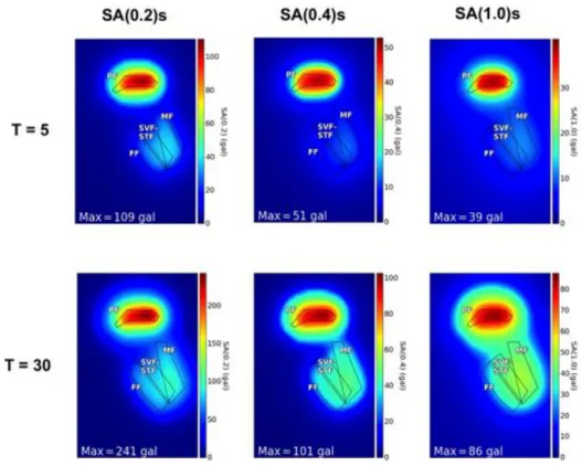
The simplest model, Level 1, is also computed for some spectral ordinates (Fig. 11) in addition to PGA values (re-ported in Figs. 9 and 10). For the spectral ordinates consid-ered, SA 0.2 s gives the highest hazard, with maximum val-ues of 109 and 241 gal for 10 % exceedance probability on exposure periods of 5 and 30 years, respectively. For all the exposure periods and spectral ordinates calculated, the haz-ard of Level 1 is dominated by PF, but note the relative in-crease of values in the southeasternmost area of the Timpe, as the spectral ordinate shifts toward lower frequencies. The results using CRISIS confirm these values and will be used for the site-specific test, given below.

Lastly, the amplification factors obtained by instrumental measures in the eastern flank of Mt. Etna have been used in CRISIS. They give the first seismic hazard site-specific maps based on real response data and clearly illustrate how ampli-fication due to local site conditions can increase the expected ground motion at rock reference sites. Even if these results are preliminary, they can be considered the first example of a new generation of site-specific seismic hazard maps suit-able for defining priorities of retrofitting at a local scale. In Fig. 12, site-amplified results at two spectral accelerations (0.2 and 1.0 s) for a 10 % probability of exceedance in 5 and 50 years are shown. The obtained values show that the site-specific conditions are by far the most important elements in driving the hazard, and the variability in ground motion alters the spatial correlations of nearby localities. Further studies will deepen these analyses by checking how we can bridge the gap existing between the probabilistic physically based models (like the study presented here) and the ones obtained

Figure 11. Hazard results of Level 1 at different spectral ordinates for a 10 % exceedance probability in 5 and 30 years, when V_s30= 800 m s 1.

Figure 12. Site-specific hazard results of Level 1 (CRISIS). In the upper panels, the maps of SA 0.2 s at 10 % exceedance probability in 5 (left panels) and 50 years (right panels) are obtained for V_s30= 800 m s 1for the whole area; the amplification factors are applied on a stripe on Mt. Etna southeastern flank (dashed black rectangle, see details in Figs. 7 and 8). The lower frames refer to SA 1.0 s.

by means of the observed intensities (Azzaro et al., 2008, 2016). By now, we acknowledge that the two approaches dif-fer mainly in the less-inhabited areas where seismic sources are defined by instrumental methods only; thus the problem

of seismic sources definition deals essentially with issues of completeness and epistemic uncertainties..

7 Conclusive remarks

This work presents the first seismic hazard maps specifically obtained for a volcano, Mt. Etna in Sicily, and the implemen-tations introduced ad hoc in two PSHA software packages (CRISIS, Ordaz et al., 2013; OpenQuake engine, Pagani et al., 2014). Results are given in terms of acceleration (PGA and spectral ordinates at 0.2, 0.4 and 1.0 s) for shorter re-turn periods than those normally used in regulation, i.e., for a 10 % exceedance probability in 5 and 30 years (correspond-ing to return periods of 47 and 284 years, respectively) as they are intended to be a tool for prioritization of risk mitiga-tion acmitiga-tions.

The main novelties introduced in this study are as follows: – The derivation and the introduction of a new GMPE

into the software account for the peculiar propagation properties in this volcanic area: it takes into account hypocentral distance (Rhypo) and is used jointly with

an original magnitude–rupture relationship (see Part 1 companion paper, Azzaro et al., 2017), derived from the Mt. Etna dataset.

– New computational capabilities in PSHA software are implemented by introducing the rough volcano topogra-phy, which both softwares benefitted from. Accounting for more realistic source-to-site distances can impact re-sults up to 50 % of the expected values for the shallow-est sources in the near field.

– The conceptual composition of seismic sources is han-dled in a framework of increasing complexity. Mt. Etna sources are depicted through an extensive analysis of geological, historical and instrumental earthquake data, described in detail in Part 1. A basic observation is that a high-quality instrumental monitoring obtained during an interseismic period of 10 years at Mt. Etna is rep-resentative of the frequency–magnitude distribution de-rived from a 2-century-long historical catalogue. This encouraged us to use the non-declustered catalogue for parameterizing the seismic sources, potentially open-ing the usage of generalized, non-Poissonian models for treating the earthquake generation processes in volcanic areas. Further studies are planned to check the applica-bility of such assumptions in other contexts.

– The seismic sources have been structured in three in-dependent layers, some of them branching to account for different parameterization (e.g., based on histori-cal or geologihistori-cal constraints, to handle the uncertainty of Mmax for a fault source) or different assumptions

(e.g., about time dependency, using Poissonian station-ary rates, or probability rates conditioned to the time elapsed since the last major event, based on simplified BPT distributions). We believe in this way the epistemic uncertainties are properly accounted for.

The hazard maps computed in our study have higher spatial resolution than the national hazard maps, and those referred to rock conditions (where Vs30= 800 m s 1, i.e., soil type A)

indicate significantly higher hazard than the ones used by regulation, even though they only consider shallow volcano-tectonic sources and do not account for the regional sources capable of releasing M > 6 earthquakes like the national haz-ard maps do. A preliminary modeling of site-specific hazhaz-ard is also attempted on the Mt. Etna’s eastern flank, where ex-tensive fieldwork has been performed for characterizing local amplification factors. They provide a new picture of expected ground motion, about twice the values assigned to reference rock sites, and are spatially uncorrelated.

We hope that these analyses will be deepened and broadened by the extensive microzonation investigations carried out in the frame of the activities promoted and funded by the Italian Department for Civil Protec-tion (e.g., http://www.protezionecivile.gov.it/jcms/it/piano_ nazionale_art_11.wp) and integrated into the regulation framework in order to have realistic and useful ground-motion prediction maps devoted to urban planners and struc-tural designers.

Finally, we hope that components of this work can be use-ful in the seismic hazard assessment of other volcanic re-gions.

Code and data availability. The implementation information of the codes CRISIS and OpenQuake is available with the current re-leases (https://sites.google.com/site/codecrisis2015/home; https:// github.com/gem/oq-engine, last accessed 30 September 2017). Other details of the source models are provided in Azzaro et al. (2017) and can be provided on demand.

The Supplement related to this article is available online at https://doi.org/10.5194/nhess-17-1999-2017-supplement.

Competing interests. The authors declare that they have no conflict of interest.

Special issue statement. This article is part of the special issue “Linking faults to seismic hazard assessment in Europe”. It is not associated with a conference.

Acknowledgements. Many thanks are due to G. Weatherill, to an anonymous reviewer and to the Guest Editor O. Scotti, for fruitful discussions and suggestions about methodological issues. This study has benefited from funding provided by the Italian Presi-denza del Consiglio dei Ministri – Dipartimento della Protezione Civile (DPC), in the framework of the 2012–2014 Agreement with Istituto Nazionale di Geofisica e Vulcanologia (INGV), projects V3 “Multi-disciplinary analysis of the relationships between tectonic

structures and volcanic activity” and S2 “Constraining observations into seismic hazard”. This paper does not necessarily represent DPC official opinion and policies.

Edited by: Oona Scotti

Reviewed by: Graeme Weatherill and one anonymous referee

References

Abe K.: Magnitudes of major volcanic earthquakes of Japan 1901 to 1925, J. Fac. Sci., Hokkaido Univ. Ser. VII, 6, 201–212, 1979. Alparone, S., Maiolino, V., Mostaccio, A., Scaltrito, A., Ursino, A., Barberi, G., D’Amico, S., Di Grazia, G., Giampiccolo, E., Musumeci, C., Scarfì, L., and Zuccarello, L.: Instrumental seismic catalogue of Mt. Etna earthquakes (Sicily, Italy): ten years (2000–2010) of instrumental recordings, Ann. Geophys., 58, S0435, https://doi.org/10.4401/ag-6591, 2015.

Azzaro, R.: Seismicity and active tectonics in the Etna region: con-straints for a seismotectonic model, in: Mt. Etna: volcano labora-tory, edited by: Bonaccorso, A., Calvari, S., Coltelli, M., Del Ne-gro, C., and Falsaperla, S., American Geophysical Union, Geo-phys. Monogr., 143, 205–220, 2004.

Azzaro, R. and De Rosa R.: Project V3. Multi-disciplinary analy-sis of the relationships between tectonic structures and volcanic activity (Etna, Vulcano-Lipari system), Final Report 1 Novem-ber 2014–30 June 2015, Agreement INGV-DPC 2012-2021, Volcanological programme 2012–2015, Miscellanea INGV, 29, 172 pp., 2016.

Azzaro, R., Barbano, M. S., Moroni, A., Mucciarelli, M., and Stuc-chi, M.: The seismic history of Catania, J. Seismol., 3, 235–252, 1999.

Azzaro, R., Barbano, M. S., D’Amico, S., Tuvè, T., Albarello, D., and D’Amico, V.: First studies of probabilistic seismic hazard as-sessment in the volcanic region of Mt. Etna (southern Italy) by means of macroseismic intensities, Bollettino di Geofisica Teor-ica e ApplTeor-icata, 49, 77–91, 2008.

Azzaro, R., Carocci, C. F., Maugeri, M., and Torrisi, A.: Micro-zonazione sismica del versante orientale dell’Etna studi di primo livello, edited by: Le nove Muse, Catania, 181 pp., 2010. Azzaro, R., D’Amico, S., Peruzza, L., and Tuvè, T.: Earthquakes

and faults at Mt. Etna (Southern Italy): problems and perspec-tives for a time-dependent probabilistic seismic hazard assess-ment in a volcanic region, Bollettino di Geofisica Teorica e Ap-plicata, 53, 75–88, 2012.

Azzaro, R., D’Amico, S., Peruzza, L., and Tuvè, T.: Probabilistic seismic hazard at Mt. Etna (Italy): the contribution of local fault activity in mid-term assessment, J. Volcanol. Geoth. Res., 251, 158–169, 2013.

Azzaro, R., D’Amico, S., and Tuvè, T.: Seismic hazard assessment in the volcanic region of Mt. Etna (Italy): a probabilistic ap-proach based on macroseismic data applied to volcano-tectonic seismicity, Bull. Earthq. Eng., 14, 1813–1825, 2016.

Azzaro, R., Barberi, G., D’Amico, S., Pace, B., Peruzza, L., and Tuvè, T.: When probabilistic seismic hazard climbs volcanoes: the Mt. Etna case, Italy – Part 1: Model components for sources parametrization, Nat. Hazards Earth Syst. Sci., 17, 1981–1998, https://doi.org/10.5194/nhess-17-1981-2017, 2017.

Barani, S. and Spallarossa, D.: Soil amplification in probabilistic ground motion hazard analysis, Bull. Earthq. Eng., 15, 2525– 2545, https://doi.org/10.1007/s10518-016-9971-y, 2016. Bindi, D., Pacor, F., Luzi, L., Puglia, R., Massa, M., Ameri, G., and

Paolucci, R.: Ground motion prediction equations derived from the Italian strong motion database, Bull. Earthq. Eng., 9, 1899– 1920, https://doi.org/10.1007/s10518-011-9313-z, 2011. Boore, D. M.: Prediction of ground motion using the stochastic

method, Pure Appl. Geophys., 160, 635–676, 2003.

Boore, D. M. and Atkinson, G. M.: Ground-motion prediction equa-tions for the average horizontal component of PGA, PGV, and 5 %-damped PSA at spectral periods between 0.01 s and 100 s, Earthquake Spectra, 24, 99–13, 2008.

Branca, S. and Ferrara, V.: The morphostructural setting of Mount Etna sedimentary basement (Italy): implica-tions for the geometry and volume of the volcano edi-fice and its flank instability, Tectonophysics, 586, 46–64, https://doi.org/10.1016/j.tecto.2012.11.011, 2013.

Branca, S., Coltelli, M., and Groppelli, G.: Geological evolution of a complex basaltic stratovolcano: Mount Etna, Italy, Ital. J. Geosci., 130, 306–317, https://doi.org/10.3301/IJG.2011.13, 2011.

D’Amico, S., Meroni, F., Sousa, M. L., and Zonno, G.: Building vulnerability and seismic risk analysis in the urban area of Mt. Etna volcano (Italy), Bull. Earthq. Eng., 14, 2031–2045, 2016. De Gori, P. and Chiarabba, C.: Qn structure of Mount Etna:

Con-straints for the physics of the plumbing system, J. Geophys. Res., 110, B05303, https://doi.org/10.1029/2003JB002875, 2005. Giampiccolo, E., D’Amico, S., Patanè, D., and Gresta, S.:

Atten-uation and Source Parameters of Shallow Microearthquakes at Mt. Etna Volcano, Italy, Bull. Seismol. Soc. Am., 97, 184–197, https://doi.org/10.1785/0120050252, 2007.

Gruppo Analisi Dati Sismici: Catalogo dei terremoti della Sicilia Orientale – Calabria Meridionale (1999–2017), INGV, Catania http://sismoweb.ct.ingv.it/maps/eq_maps/sicily/catalogue.php, last access: 30 September 2017.

Herak, M.: ModelHVSR-A Matlab®tool to model horizontal-to-vertical spectral ratio of ambient noise, Comput. Geosci., 34, 1514–1526, 2008.

Imperatori, W. and Mai, P. M.: The role of topography and lateral velocity heterogeneities on near-source scattering and ground-motion variability, Geophys. J. Int., 202, 2163–2181, https://doi.org/10.1093/gji/ggv281, 2015.

Joyner, W. B. and Boore, M.: Peak horizontal acceleration and ve-locity from strong-motion records including records from the 1979 Imperial Valley, California, earthquake, Bull. Seismol. Soc. Am., 71, 2011–2038, 1981.

Konno, K. and Ohmachi, T.: Ground-motion characteristics esti-mated from spectral ratio between horizontal and vertical com-ponents of microtremor, Bull. Seismol. Soc. Am., 88, 228–241, 1998.

Langer, H., Tusa, G., Scarfì, L., and Azzaro, R.: Ground-motion scenarios on Mt. Etna inferred from empirical relations and syn-thetic simulations, Bull. Earthq. Eng., 14, 1917–1943, 2016. Lermo, J. and Chavez-Garcia, F. J.: Site effect evaluation using

spectral ratios with only one station, Bull. Seismol. Soc. Am., 83, 1574–1594, 1993.

Lombardo, G., Langer, H., Gresta, S., Rigano, R., Monaco, C., and De Guidi, G.: On the importance of

geolithologi-cal features for the estimate of the site response: the case of Catania metropolitan area (Italy), Nat. Hazards, 38, 339–354, https://doi.org/10.1007/s11069-005-0386-3, 2006.

Longo, E.: Seismic input modelling for relevant earthquakes in Eastern Sicily, PhD thesis, University of Malta, Malta, 190 pp., 2017.

Nakamura, Y.: A method for dynamic characteristics estimation of sub surface using microtremor on the surface, Railw. Tech. Res. Inst. Rep. 30, Railway Technical Research Institute, Tetsudo, Gi-jutsu, Kenkyujo, 25–33, 1989.

Nogoshi, M. and Igarashi, T.: On the amplitude characteristic of mi-crotremor (part 2) (in Japanese with English abstract), J. Seismol. Soc. Jpn., 24, 26–40, 1971.

Ordaz, M., Martinelli, F., and D’Amico, V., and Meletti, C.: CRI-SIS2008: A flexible tool to perform probabilistic seismic hazard assessment, Seismol. Res. Lett., 84, 495–504, 2013.

Pace, B., Visini, F., and Peruzza, L.: FiSH: MATLAB tools to turn fault data into seismic hazard models, Seismol. Res. Lett., 87, 374–386, https://doi.org/10.1785/0220150189, 2016.

Panzera, F., Rigano, R., Lombardo, G., Cara, F., Di Giulio, G., and Rovelli, A.: The role of alternating outcrops of sediments and basaltic lavas on seismic urban scenario: the study case of Cata-nia, Italy, Bull. Earthq. Eng., 9, 411–439, 2011.

Pagani, M., Monelli, D., Weatherill, G., Danciu, L., Crow-ley, H., Silva, V., Henshaw, P., Butler, L., Nastasi, M., Panzeri, L., Simionato, M., and Viganò, D.: OpenQuake-engine: An open hazard (and risk) software for the Global Earthquake Model, Seismol. Res. Lett., 85, 692–702, https://doi.org/10.1785/0220130087, 2014.

Panzera, F., Lombardo, G., and Muzzetta, I.: Evaluation of the buildings fundamental period through in-situ experimental tech-niques in the urban area of Catania, Italy, Phys. Chem. Earth, 63, 136–146, https://doi.org/10.1016/j.pce.2013.04.008, 2013. Panzera, F., Lombardo, G., Monaco, C., and Di Stefano, A.:

Seis-mic site effects observed on sediments and basaltic lavas out-cropping in a test site of Catania, Italy, Nat. Hazards, 79, 1–27, https://doi.org/10.1007/s11069-015-1822-7, 2015.

Panzera, F., Sicali, S., Lombardo, G., Imposa, S., Gresta, S., and D’Amico, S.: A microtremor survey to define the sub-soil structure in a mud volcanoes area: the case study of Salinelle (Mt. Etna, Italy), Environm. Earth Sci., 75, 1140, https://doi.org/10.1007/s12665-016-5974-x, 2016.

Panzera, F., Lombardo, G., Longo, E., Langer, H., Branca, S., Az-zaro, R., Cicala, V., and Trimarchi, F.: Exploratory seismic site response surveys in a complex geologic area: a case study from Mt. Etna volcano (southern Italy), Nat. Hazards, 86, 385–399, https://doi.org/10.1007/s11069-016-2517-4, 2017.

Patanè, D., Ferrucci, F., and Gresta, S.: Spectral features of mi-croearthquakes in volcanic areas: attenuation in the crust and am-plitude response of the site at Mt. Etna, Italy, Bull. Seismol. Soc. Am., 84, 1842–1860, 1994.

Peruzza, L., Gee, R., Pace, B., Roberts, G., Scotti, O., Visini, F., Benedetti, L., and Pagani, M.: PSHA after a strong earthquake: hints for the recovery, Ann. Geophys., 59, 1–9, https://doi.org/10.4401/ag-7257, 2016.

Priolo, E.: 2-D spectral element simulation of destructive ground shaking in Catania (Italy), J. Seismol., 3, 289–309, 1999. Rahpeyma, S., Halldorsson, B., Oliveira, C. S., Green, R. A.,

and Jónsson, S.: Detailed site effect estimation in the pres-ence of strong velocity reversals within a small-aperture strong-motion array in Iceland, Soil Dynam. Earthq. Eng., 89, 136–151, https://doi.org/10.1016/j.soildyn.2016.07.001, 2016.

Saraò, A., Cocina, O., Moratto, L., and Scarfì, L.: Earthquake fea-tures through the seismic moment tensor, in: Project V3 – Multi-disciplinary analysis of the relationships between tectonic struc-tures and volcanic activity (Etna, Vulcano-Lipari system): Final Report (1 November 2014–30 June 2015), Agreement INGV-DPC 2012-2021, Volcanological Programme 2012–2015, edited by: Azzaro R. and De Rosa, R., Miscellanea INGV, 29, 98–102, 2016.

Schnabel, P. B., Lysmer, J., and Seed, H. B.: Shake a computer program for earthquake response analysis of horizontally lay-ered sites, Report No. EERC 72-12, Earthquake Engineering Research Center, University of California, Berkeley, California, 1972.

SESAME: Guidelines for the implementation of the H/V spectral ratio technique on ambient vibrations: Measure-ments, processing and interpretation, SESAME European Research Project WP12, deliverable D23.12, availabe at: ftp://ftp.geo.uib.no/pub/seismo/SOFTWARE/SESAME/ USER-GUIDELINES/SESAME-HV-User-Guidelines.pdf (last access: 30 September 2017), 2004.

Sicali, S., Barbano, M. S., D’Amico, S., and Azzaro, R.: Charac-terization of seismicity at Mt. Etna volcano (Italy) by inter-event time distribution, J. Volcanol. Geoth. Res., 270, 1–9, 2014. Stucchi, M., Meletti, C., Montaldo, V., Crowley, H., Calvi, G. M.,

and Boschi, E.: Seismic Hazard Assessment (2003–2009) for the Italian Building Code, Bull. Seismol. Soc. Am., 01, 1885–1911, https://doi.org/10.1785/0120100130, 2011.

Tusa, G. and Langer, H.: Prediction of ground-motion parame-ters for the volcanic area of Mount Etna, J. Seismol., 20, 1–42, https://doi.org/10.1007/s10950-015-9508-x, 2016.

Yokoyama, I.: The largest magnitudes of earthquakes associated with some historical volcanic eruptions and their volcanological significance, Ann. Geophys., 44, 1021–1029, 2001.

Zobin, V. M.: Seismic hazard of volcanic activity, J. Volcanol. Geoth. Res., 112, 1–14, 2001.

Zobin, V. M.: Introduction to Volcanic Seismology, 2nd Edn., Else-vier, Amsterdam, New York, Tokyo, 482 pp., 2012.