Alma Mater Studiorum – Università di Bologna
DOTTORATO DI RICERCA IN
Ingegneria biomedica, elettrica e dei sistemi (IBES),
curriculum ingegneria elettrica
Ciclo XXX
Settore Concorsuale: 09/E2 Ingegneria dell’energia elettrica
Settore Scientifico Disciplinare: ING-IND 32 Convertitori, macchine e azionamenti elettrici
TITOLO TESI
MULTIPHASE ELECTRIC DRIVES FOR “MORE ELECTRIC
AIRCRAFT” APPLICATIONS
Presentata da:
Giacomo Sala
Coordinatore Dottorato
Supervisore
Prof. Daniele Vigo
Prof. Angelo Tani
i
I want to thank a lot Angelo Tani for having taught me the research method and for his kind supervision.
Thanks to my colleagues from Bologna and Nottingham universities for helping me to solve everyday problems.
i
Index
Index ... i
List of Figures ... ix
List of Tables ... xxi
Introduction ... xxiii
... 1
Multiphase Machines for More Electric Aircraft applications ... 1
Aircraft Industry and Market ... 1
The idea of More Electric Aircraft ... 3
The idea of More Electric Engine... 5
Embedded starter/generator location ... 6
Embedded starter/generator machine topologies ... 7
State of the Art and Applications of Multiphase Drives ... 9
Performance ... 10
Fault tolerance and diagnosis ... 11
New control techniques ... 13
Multiphase Machines as a Fault-Tolerant solution for MEA applications ... 13
Multi-Harmonic Generalised Model for Multiphase Machines ... 25
Space Vector Decomposition theory ... 26
Space Vectors Transformation (odd number of variables) ... 28
Space Vectors Transformation (even number of variables) ... 29
General approach to Multiphase Machine Modelling: Stator Winding and Transformations ... 31
Armature field (one turn) ... 32
Armature field (multiphase winding) ... 39
Space vectors analysis for modelling of multiphase machines ... 41
Space vectors analysis (the standard three-phase winding) ... 44
Space vectors analysis (12 phase asymmetrical winding) ... 48
Space vectors analysis (nine phase winding) ... 50
Space vectors analysis (multi-sectored triple three-phase winding) ... 53
ii
Voltage equation (single turn) ... 56
Voltage equation (single phase) ... 57
Voltage equation (multiphase winding) ... 58
Linked Flux Space Vectors ... 61
Linked flux (single turn) ... 61
Linked flux (single phase) ... 63
Linked flux (multiphase winding) ... 64
Self inductance (single turn) ... 65
Self inductance (multiphase winding) ... 66
Surface Permanent Magnet Machine Modelling ... 67
Single permanent magnet model and basic equations ... 67
Surface Permanent Magnet rotor ... 71
Voltage equation (single turn) ... 73
Voltage equation (multiphase winding) ... 74
Squirrel Cage Modelling ... 75
Squirrel cage as an Nb-phase symmetrical winding ... 76
Voltage equation (single equivalent phase - between two bars) ... 77
Voltage equation (equivalent multiphase winding of the squirrel cage) ... 78
Voltage equation (equivalent multiphase winding of a symmetrical cage) ... 81
Linked flux (general) ... 82
Self inductance (equivalent multiphase winding of a squirrel cage - SVD) ... 83
Mutual flux (effect of a single turn on the squirrel cage) ... 84
Mutual flux (effect of a multiphase winding on the squirrel cage) ... 85
Voltage equation (effect of the cage on a single turn) ... 88
Voltage equation (effect of the cage on a multiphase winding) ... 89
Voltage equations (summary) ... 91
Power, Torque and Force Equations ... 94
Power equation (single turn) ... 94
Power equation (multiphase winding) ... 97
Power equation (squirrel cage) ... 106
Airgap magnetic coenergy (alternative method for the torque evaluation) ... 113
Radial Force ... 119
Summary and Advantages of a Multi-Harmonic Model for Multiphase Machines 122 Advantages of a multi-harmonic SVD model ... 122
iii
Multi-harmonic models (summary of the equations – simplified model) ... 124
Open Phase Faults and Fault Tolerant Controls in Multiphase Drives ... 129
Open Phase faults in Electrical Drives ... 129
Open Phase Faults in Inverter Fed Multiphase Machines ... 131
Terminal Box and Converter Connection Faults ... 131
Protections and Drives ... 131
Zero Current Control and Uncontrolled Generator Behaviour ... 134
Modelling and Fault Tolerant Control for Open Phase Faults ... 135
Model of and Open Phase Fault ... 135
Open Phase Fault Tolerant Control (FTC) Concept ... 136
Open Phase Fault in Three-Phase Electrical Drives ... 136
Open Phase Fault Tolerant Control in Multiphase Electrical Drives ... 137
Optimized FTC algorithm by means of the Lagrange multipliers method ... 139
Current Sharing and Fault Tolerant Control for Independently Star Connected Multi Three-Phase Machines under Open Phase Faults ... 142
Current Sharing for Independently Star Connected Three-Phase Subsystems ... 143
Current Sharing for Independently Star Connected Three-Phase Subsystems (d-q axis control enhancement) ... 146
Open Phase FTC Algorithm for Independently Star Connected Three-Phase Subsystems ... 147
Improved Fault Tolerant Control for Multiphase Machines under Open Phase Faults 149 Optimized FTC Algorithm by means of the Lagrange Multipliers method for Multi Independently Star Connected n-Phase Subsystems (n odd) ... 149
Optimized FTC Algorithm by means of the Lagrange Multipliers method for Multi Three-Phase Subsystems Connected to a Single Star ... 150
Optimized FTC Algorithm by means of the Lagrange Multipliers method for Multi-Star Connected Three-Phase Subsystems ... 153
Optimized Open Phase FTC Algorithm for a dual three-phase winding (star connection constraints) ... 155
Optimized Open Phase FTC Algorithm for a triple three-phase winding (star connection constraints) ... 157
Optimized Open Phase FTC Algorithm for a quadruple three-phase winding (star connection constraints) ... 161
Summary of the proposed Fault Tolerant Control for Open Phase Faults ... 168
Case study: 12-Phase Asymmetrical Machine ... 171
iv
Control Schemes - Comparison ... 185
Numerical simulation results (Matlab-Simulink) ... 188
Finite Element Results (Flux): Comparison of iron saturation and related torque reduction in case of two three-phase subsystem open phase fault (best double six-phase configuration for simplified six-phase FTC performance enhancement) ... 199
Experimental results ... 203
Conclusions ... 213
High Resistance and Interturn Short Circuit Faults ... 215
Introduction to High Resistance (HR) and Interturn Short Circuit (ISC) Faults ... 216
Equivalent circuit for High Resistance and Interturn Short Circuit Faults ... 217
Circuital representation of HR and ISC faults ... 218
ISC faults – leakage inductances analysis ... 220
HR and ISC faults – resistances analysis ... 223
Circuital phase voltage equations for HR and ISC faults ... 226
Linked fluxes equations for HR and ISC faults ... 230
Interturn Short Circuit Faults: Electromagnetic Analysis of the Short Circuit Loop 232 Magnetic field generated by the ISC loop current ... 232
HR and ISC fault armature equations - Summary ... 233
Torque and radial force evaluation for ISC faults ... 235
Space Vector Model of a Multiphase Machine with a High Resistance or Interturn Short Circuit Fault ... 238
General Interturn Short Circuit with High Resistance Fault in Multiphase Electrical Machines ... 243
Summary of the complete Space Vector model for HR and ISC faults in multiphase machines ... 244
Principle for High Resistance and Interturn Short Circuit Faults Detection with Ideal Current Control (FOC) in distributed winding Induction Machines ... 246
Simplified model for distributed multiphase windings ... 247
Detection algorithm: concept ... 249
High Resistance Fault Detection Algorithm with Ideal Current Control (FOC) ... 251
Advantages of redundant equations in the HR detection algorithm for improved accuracy ... 252
High Resistance Faults in Symmetrical Multiphase Machines (odd phases) ... 256
v
Interturn Short Circuit Fault Detection with Ideal Current Control in Multiphase
Machines ... 263
Simplified model for distributed multiphase windings – space couplings caused by ISC fault in squirrel cage Induction Machines ... 264
Simplified model for distributed multiphase windings – space couplings caused by ISC fault in SPM machines with sinusoidal MMF of the rotor magnets ... 265
Interturn Short Circuit Fault Detection Algorithm with Ideal Current Control in Three-Phase Squirrel Cage Induction Machines ... 267
Simplified model for ISC fault detection in Three-Phase IMs ... 267
Simplified model for ISC fault detection in Three-Phase IMs at steady state conditions ... 268
Analytical and Experimental Results: High Resistance and Interturn Short Circuits in Three-phase Induction Machines with V/f Control ... 274
Test rig and prototype ... 275
Healthy Machine ... 277
High Resistance faults ... 281
Interturn Short Circuit faults ... 283
High Resistance and Interturn Short Circuit faults: Comparison with V/f control ... 287
Analytical Results of ISC fault detection for Three-phase IMs ... 289
Analytical and Experimental Results of High Resistance Detection in Nine-Phase Induction Machines ... 296
High Resistance Fault Detection ... 297
Conclusion ... 303
Modelling of Multi Three-Phase Sectored Machines for Radial Force Control 305 Multi Sector Permanent Magnet machines (MSPM) as a possible multiphase machine solution for radial force control ... 306
Modelling of Multi Three-Phase Sectored Stator Windings ... 307
General SVD model – additional transformation ... 307
General SVD model – Voltage equations for MSPM machines ... 312
MSPM particular SVD model – Voltage equations for MSPM machines ... 313
General SVD model – Torque and Force for MSPM machines ... 315
Modelling of a Triple Three-Phase Sectored Machine (three pole pairs) ... 320
SVD transformation – Current space vectors ... 320
Triple Three-Phase MSPM machine – Voltage Equations by General Method (redundant) ... 322
vi
Triple Three-Phase MSPM machine – Torque and Force ... 325
Force and Torque Control of a Triple Three-Phase Sectored Machine ... 331
Control equations (multi synchronous reference frames) ... 331
Radial Force Control: F2/F ratio (F2pu) ... 332
Triple Three-Phase Inverse Transformation: From the multiphase space vectors to the three-phase ones ... 334
Force Control of a Triple Three-Phase Sectored Machine: optimised control for minimum stator copper Joule losses ... 336
Current Sharing Technique for Triple Three-Phase Machines (Radial Force Control and Compensation) ... 339
Radial Force Evaluation in case of Current Sharing Control (standard method) ... 339
Current Sharing advanced control of MSPM machines and Radial Force control ... 342
Radial Force FTC in case of Three-Phase Open Phase Fault ... 346
Radial Force Equation in case of Three-Phase Open Fault (independent 3rd space control) ... 347
Radial Force Compensation in case of Three-Phase Open Fault (F=0) ... 351
Radial Force FTC in case of Three-Phase Open Fault – optimised algorithm ... 351
Finite Element Simulation Results (Magnet software)... 354
Torque and Radial Force control parameters (KT,KPM 3,2 and KPM 3,4 ) ... 355
Torque and Radial Force control (optimised control): ... 356
Radial Force Evaluation in case of Three-Phase Open Fault (standard torque control) 363 Radial Force Compensation at Rated Torque (id3=0 FTC) ... 364
Radial Force Fault Tolerant Control at Rated Torque (id3=0 FTC) – constant force .... 366
Radial Force Fault Tolerant Control at Rated Torque (id3=0 FTC) – direction criticality ... 369
Numerical (Matlab-Simulink) Simulation Results ... 370
Radial Force Open Loop Control ... 372
Radial Force Open Loop Compensation (With detection delay) ... 374
Radial Force Open Loop Compensation (instantaneous) ... 376
Bearingless Operation and FTC (early compensation) – rated torque and rated force .. 378
Bearingless Operation and optimised current sharing control – rated torque and rated force ... 381
Bearingless Operation with Optimised FTC – Minimum copper Joule losses ... 383
Experimental Results ... 386
vii
Radial Force Control in Bearingless Closed Loop Operation (stand still) ... 390
Radial Force Control in Bearingless Closed Loop Operation (rated speed - 3000 rpm) 392 Radial Force Control in Bearingless Closed Loop Operation (transient up to 3000 rpm) ... 394
Radial Force Control in Bearingless Closed Loop Operation (bearingless control activation at 1000 rpm) ... 396
Conclusions ... 399
Design and Control of Segmented Multi Three-Phase SPM Machines ... 403
Sectored and Segmented motor design - Concept ... 404
Summary of the Segmentation Design Degrees of Freedom ... 406
Field Analysis of a Triple Three-phase Sectored and Segmented SPM ... 407
General SV model of a segmented and sectored machine ... 408
SV Model of a Triple Three-Phase Segmented and Sectored SPM Machine ... 411
Machine Control and Winding Design ... 413
Torque Ripples in Segmented Machines ... 416
New Winding Design for Standard Current Control ... 418
Segmented Machine Control Technique for Standard Windings Designs ... 419
Coil Pitch, End Effect and Cogging Torque in Segmented Sectored Machines ... 420
Coil Pitch ... 420
End Effect and Cogging Torque ... 422
FEA Simulation Results ... 423
Performance - Healthy Machine Behaviour ... 423
Fault Tolerant Behaviour ... 430
Machine Prototype and Thermal Analysis ... 431
Machine Design ... 432
Thermal Analysis for Future Developments ... 434
Conclusion ... 438
Abstract ... i
Academic activities ... ii
Summary of the research activity ... ii
Seminars ... iii
Research period abroad ... iii
Assistant Supervisor ... iv
ix
List of Figures
Fig. 1.1– Power flow in a standard civil aircraft. ... 3
Fig. 1.2 – Power flow in a civil MEA. ... 4
Fig. 1.3 – The MEA concept on Boeing 787. ... 5
Fig. 1.4 – Rolls-Royce electric starter/generator embedded in the gas turbine engine. ... 6
Fig. 1.5 – Operating temperatures in a typical jet engine. ... 7
Fig. 1.6 – A typical MEE layout. ... 8
Fig. 1.7 - Multiphase system connected to a standard three-phase grid. ... 9
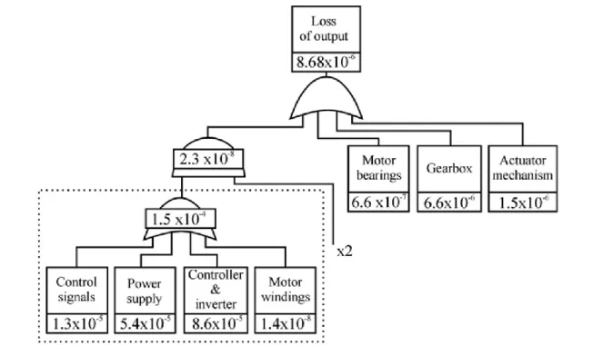
Fig. 1.8 - Single channel electromecchanical actuator fault-tree (probabilities given per hour flight). ... 14
Fig. 1.9 - Dual-lane electromecchanical actuator fault-tree (probabilities given per hour flight). ... 15
Fig. 1.10 - Method of flight control redundancy. ... 15
Fig. 1.11 - Redundancies of multiphase machines. ... 16
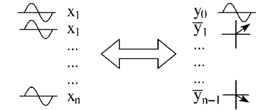
Fig. 2.1 – Space vector transformation and inverse transformation of an n variable system. . 26
Fig. 2.2 – Conventions of the proposed model. ... 34
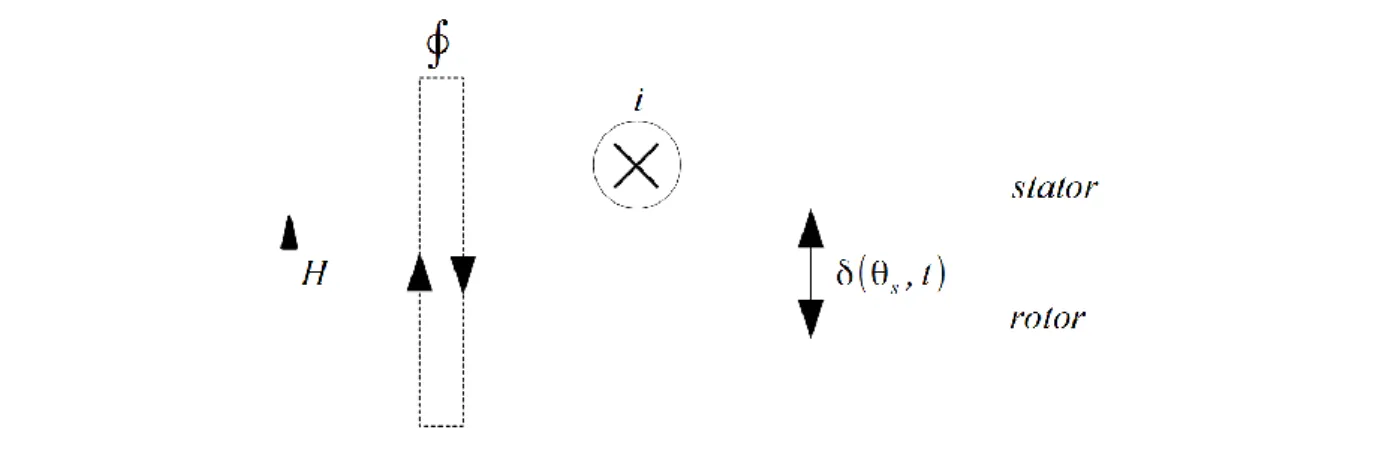
Fig. 2.3 – Spatial location of a turn (turn k) in the airgap circumference. ... 34
Fig. 2.4 – Spatial location of a turn (turn k) in the airgap circumference. ... 35
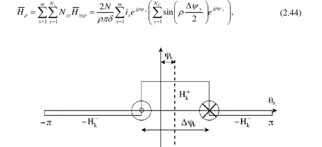
Fig. 2.5 – Spatial distribution of the magnetic field produced by a turn (turn k) in the airgap. ... 39
Fig. 2.6 – Six slots distributed winding three-phase machine concept (example). The green vertical line (magnetic axis of the first phase) highlights the origin of the stator reference frame. ... 44
Fig. 2.7 – Six slots distributed winding three-phase machine with asymmetrical (left) and symmetrical (right) winding distribution (concept). With “x” are indicated the starting slots of the phases and with “o” the final ones. ... 45
Fig. 2.8 – 48 slots and 2 pole pairs distributed winding 12-phase machine. Asymmetrical winding (left) and quadruple three-phase winding (right). The magnetic axis and the starting of the phases are highlighted with coloured lines in the back iron and with crosses in the slots respectively. ... 48
Fig. 2.9 – 36 slots and 2 pole pairs distributed winding 9-phase machine. Asymmetrical winding (left) and symmetrical winding (right). The magnetic axis and the starting of the phases are highlighted with coloured lines in the back iron and with crosses in the slots respectively. Note: the winding on the right is symmetrical in its electrical degrees representation. ... 51
Fig. 2.10 – 18 slots and 3 pole pairs sectored winding 9-phase machine. The magnetic axis and the starting of the phases in the first sector are highlighted with coloured lines in the back iron and with crosses in the slots respectively. ... 54
Fig. 2.11 – Simplified magnetic behaviour of the magnets. ... 67
Fig. 2.12 – Magnet with constant radial thickness with a general machine reluctance. ... 68
Fig. 2.13 - SPM rotor with three pole pairs. ... 71
Fig. 2.14 - Squirrel cage and related model parameters. ... 76
x
Fig. 2.16 – Electrical circuit and parameters of the equivalent phase of a squirrel cage. ... 78
Fig. 2.17 - Example of B-H curve of a high power density hard magnetic material. ... 114
Fig. 2.18 - Coenergy of a hard magnetic material (concept). ... 115
Fig. 3.1 – Open phase faults in a standard three-phase drive (most typical faults). ... 130
Fig. 3.2 – Single switching open fault scheme in case of a top driver protections or missing signal from the DSP fault. Transient behaviour of the fault with a positive current (left) and steady state behaviour (right). ... 132
Fig. 3.3 – Single switching open fault scheme in case of a bottom driver protections or missing signal from the DSP fault. Transient behaviour of the fault with a positive current (left) and steady state behaviour (right). ... 134
Fig. 3.4 – Schematic draw of the three-phase subsystem FTC. a) and b) show example of not optimized current controls, while c) shows the solution with the phase of the inverter current contributions that minimizes the stator Joule losses to maintain the sameiS1value for a quadruple three-phase systems (NT=4). ... 144
Fig. 3.5 – Logic for the fault protection on a single leg. ... 147
Fig. 3.6 – Full three-phase fault protection logic. ... 148
Fig. 3.7 – Typical star configurations for a quadruple three-phase winding. ... 150
Fig. 3.8 – Double three-phase standard drive and relative magnetic axis directions. ... 155
Fig. 3.9 – Triple three-phase standard drive and relative magnetic axis directions. ... 158
Fig. 3.10 – Quadruple three-phase standard drive and relative magnetic axis directions. ... 162
Fig. 3.11 – Schematic of a standard quadruple three-phase drive and magnetic axis directions of the 12-phase machine. ... 171
Fig. 3.12 – Schematic of the basic idea of the three-phase FTC (purple) and the single-phase FTC (green) in case of single phase open fault for an independent star configuration of a multi three-phase machine. ... 172
Fig. 3.13 – Analytical Joule losses comparison of the healthy machine (blue) and the faulty machine (phase A1 open), with three-phase FTC (purple) and single-phase FTC (green). .. 173
Fig. 3.14 – Analytical maximum phase current comparison of the healthy machine (blue) and the faulty machine (phase A1 open), with three-phase FTC (purple) and single-phase FTC (green). ... 174
Fig. 3.15 – Analytical Joule losses comparison with healthy machine (blue) and the faulty machine (phase A1 open). Three-phase FTC (purple) and single-phase FTC: quadruple three-phase layout (green), double six-three-phase layouts (spotted) and twelve-three-phase layout (orange). The rated copper Joule losses are highlighted in red. ... 175
Fig. 3.16 – Analytical maximum phase current comparison with healthy machine (blue) and the faulty machine (phase A1 open). Three-phase FTC (purple) and single-phase FTC: quadruple three-phase layout (green), double six-phase layouts (spotted) and twelve-phase layout (orange). The maximum phase current is highlighted in red. ... 175
Fig. 3.17 – Analytical phase currents at rated value of the main current space vector. Healthy machine. ... 176
Fig. 3.18 – Analytical phase currents at rated value of the main current space vector. Three-phase FTC (Three-phase A1 open). ... 177
Fig. 3.19 – Analytical phase currents at rated value of the main current space vector. Single-phase FTC (Single-phase A1 open). ... 177
xi
Fig. 3.20 – Analytical phase currents at rated value of the main current space vector. Double
six-phase layout AB|CD (phase A1 open). ... 178
Fig. 3.21 – Analytical phase currents at rated value of the main current space vector. Double six-phase layout AC|BD (phase A1 open). ... 178
Fig. 3.22 – Analytical phase currents at rated value of the main current space vector. Double six-phase layout AD|BC (phase A1 open). ... 179
Fig. 3.23 – Analytical phase currents at rated value of the main current space vector. Twelve-phase layout ABCD ... 179
Fig. 3.24 – Analytical Joule losses comparison with healthy machine (blue) and the faulty machine (phases A1, B1, B2, D1, D2 open). Three-phase FTC (purple) and single-phase FTC: quadruple three-phase layout (green), double six-phase layouts (spotted) and twelve-phase layout (orange). The rated copper Joule losses are highlighted in red. ... 180
Fig. 3.25 – Analytical maximum phase current comparison with healthy machine (blue) and the faulty machine (phases A1, B1, B2, D1, D2 open). Three-phase FTC (purple) and single-phase FTC: quadruple three-phase layout (green), double six-phase layouts (spotted) and twelve-phase layout (orange). The maximum twelve-phase current is highlighted in red. ... 181
Fig. 3.26 – Analytical phase currents at rated value of the main current space vector. Healthy machine. ... 181
Fig. 3.27 – Analytical phase currents at rated value of the main current space vector. ... 182
Fig. 3.28 – Analytical phase currents at rated value of the main current space vector. ... 182
Fig. 3.29 – Analytical phase currents at rated value of the main current space vector. ... 183
Fig. 3.30 – Analytical phase currents at rated value of the main current space vector. ... 183
Fig. 3.31 – Analytical phase currents at rated value of the main current space vector. ... 184
Fig. 3.32 – Analytical phase currents at rated value of the main current space vector. ... 184
Fig. 3.33 – Block diagram of the current sharing and three-phase FTC control scheme. ... 186
Fig. 3.34 – Block diagram of the single-phase and three-phase FTC control schemes. ... 187
Fig. 3.35 – Block diagram of the single-phase and three-phase FTC control schemes. ... 188
Fig. 3.36 – Simulation of a speed transient from 0 to 300 rpm, followed by the fault of phase A1 open (t=1s). From 1 to 1.25 s three-phase subsystem FTC, from 1.25 to 1.5 s single-phase FTC. The last subplot shows the α−β components of the main current space vector iS1 (blue) and of the auxiliary ones (red). ... 189
Fig. 3.37 – Simulated phase currents. The machine is healthy (top left) and then has phase A1 opened, with the three-phase FTC (top right) and the single-phase FTC (centre and bottom). With colours are differentiated the 1st phase (blue), the 2nd (green) and the 3rd (orange) of each inverter. The thickest lines refer to the phase currents of inverter A. ... 190
Fig. 3.38 – Simulated current space vectors trajectories. Trajectory of iS1 (blue) and of the auxiliary vectors in case of single-phase FTC (green) and three-phase subsystem FTC (purple). ... 191
Fig. 3.39 – Three-phase homopolar currents in case of phase A1 open fault and single phase FTC. AB|CD star connection (top), AC|BD star connection (centre) and AD|BC star connection (bottom). ... 193
Fig. 3.40 – Three-phase homopolar currents in case of phase A1 open fault and single phase FTC. Single-star layout. ... 196
xii
Fig. 3.42 – Flux view for the healthy machine (left), the machine working with a three-phase open fault without FTC (centre) and with three-phase FTC (right). Inverter D three-phase open fault. ... 200 Fig. 3.43 – Flux view for the healthy machine (left), the machine working with a six-phase open fault without FTC (centre) and with six-phase FTC (right). Inverters C and D six-phase open fault. ... 201 Fig. 3.44 – Flux view for the healthy machine (left), the machine working with a six-phase open fault without FTC (centre) and with six-phase FTC (right). Inverters B and D six-phase open fault. ... 202 Fig. 3.45 – Test bench. From left to right: load (bidirectional drive) gearbox 9:1, torque meter, scaled prototype. ... 203 Fig. 3.46 – Test bench. From the left to the right: DSP TMS320F28335, control board (with DSP), driver’s board for one three-phase winding, power board for one three-phase winding. ... 204 Fig. 3.47 – Quadruple three-phase inverter (left) and twelve phase starter/generator scaled prototype (right). ... 204 Fig. 3.48 – Matryoshka current sharing control with
K
A
2
K
B
4
K
C
8
K
D, [10 A/div]. 205 Fig. 3.49 – Simplified current sharing control with KA 0.5 andK
B
K
C
K
D
0
.
5
, [10 A/div]. ... 205 Fig. 3.50 – Measured currents of the inverter-B, when the machine is healthy (top left) and then has phase A1 opened, with the three-phase subsystem FTC (top right). Then all the inverter currents with the single-phase FTC are shown: inverter-A (centre left), inverter-B (centre right), inverter-C (bottom left), inverter-D (bottom right). With colours are differentiated the 1st phase(blue), the 2nd (green) and the 3rd (orange) of each inverter, [2A/div]. ... 207 Fig. 3.51 – Measured current space vectors trajectories. Trajectory of (left) and of the auxiliary vectors (5th, 7th and 11th from the left to the right) in case of single-phase FTC (top)
and three-phase subsystem FTC (bottom), [2A/div]. ... 207 Fig. 3.52 – Total stator copper Joule losses in case of phase A1 open fault with three-phase FTC (left) and single-phase FTC (right), [ 20W/div]. ... 208 Fig. 3.53 – Three-phase homopolar currents in case of phase A1 open fault and single-phase FTC. AB|CD star layout, [2A/div]. ... 208 Fig. 3.54 – Three-phase homopolar currents in case of phase A1 open fault and single-phase FTC. AC|BD star layout, [2A/div]. ... 209 Fig. 3.55 – Three-phase homopolar currents in case of phase A1 open fault and single-phase FTC. AD|BC star layout, [2A/div]. ... 209 Fig. 3.56 – Three-phase homopolar currents in case of phase A1 open fault and single phase FTC. Single-star layout, [2A/div]. ... 211 Fig. 4.1 – High resistance (left) and Interturn short circuit (right) faults. Concept. ... 216 Fig. 4.2 – Ideal Interturn short circuit fault (left) and equivalent circuit (right). Concept. .... 217 Fig. 4.3 – High Resistance and Interturn Short Circuit concept and proposed nomenclature. Phase x (bottom) is healthy; phase y (centre) is affected by a HR condition; phase z (top) is affected by an ISC fault (with a resulting possible resistance variation). ... 218
1
S
xiii
Fig. 4.4 – Interturn Short Circuit concept and proposed nomenclature. Phase z is affected by an ISC fault (with a resulting possible resistance variation), and all the slot leakage effects are represented by their respective constants in case of a single slot pair per phase winding. .... 220 Fig. 4.5 – Interturn Short Circuit concept and proposed nomenclature for the leakage flux analysis. Phase x is healthy; phase z1 is affected by an ISC in the end winding; phase z2 is affected by a slot ISC fault. ... 221 Fig. 4.6 – Interturn Short Circuit concept and proposed nomenclature for the resistances analysis. Phase x is healthy; phase z1 is affected by an ISC in the end winding; phase z2 is affected by a slot ISC fault. With “Q” are highlighted the main radial thermal paths related to the short circuit current copper Joule losses (the axial path is implicit). ... 224 Fig. 4.7 – Three-phase IM BA 112 MB4 from M.G.M. Motori Elettrici S.p.A (left) and winding scheme (right). ... 275 Fig. 4.8 – Rewinding process from the original three-phase machine to the new customized winding. ... 276 Fig. 4.9 - New prototype of nine phase IM and test rig (left top), new winding scheme (right) and electrical winding scheme of the phase U1, where the are many additional terminals for interturn short circuit tests (left bottom). ... 276 Fig. 4.10 - Matlab-Simulink simulation V/f control with healthy machine. Phase currents (red, blue and green) and short circuit current (purple) at the top; current space vector trajectory at the bottom. ... 278 Fig. 4.11 - Drive used for the V/f experimental tests on the prototype in its three-phase winding configuration. Control board (left) and inverter (right). The DSP of the control board is a TMS320F2812. ... 279 Fig. 4.12 - Test setup scheme (top), terminal box connections for three-phase winding configuration and setup for the ISC and HR tests (bottom). ... 279 Fig. 4.13 - Experimental tests V/f control with healthy machine. Phase currents (red, blue and green) and short circuit current (purple) at the top; Current space vector trajectory at the bottom. ... 280 Fig. 4.14 - Matlab-Simulink simulation V/f control with High Resistance fault (1.85 Ohm additional) in the mentioned phases. Current space vector trajectories [2A/div]. ... 281 Fig. 4.15 - Experimental results V/f control with High Resistance fault (1.85 Ohm additional) in the mentioned phases. Current space vector trajectories [2A/div]. ... 282 Fig. 4.16 - Matlab-Simulink simulation V/f control with Interturn Short Circuit fault at no load (1.85 Ohm short circuit resistance) in the mentioned phases and coils. Current space vector trajectories [2A/div]. ... 283 Fig. 4.17 - Matlab-Simulink simulation V/f control with Interturn Short Circuit fault on the U phase at no load (top), 10 Nm (centre) and 20 Nm (bottom) (1.85 Ohm short circuit resistance) in the mentioned phases and coils. Phase currents (red, blue and green) and short circuit current (purple). ... 284 Fig. 4.18 - Experimental results V/f control with Interturn Short Circuit fault at no load (1.85 Ohm short circuit resistance) in the mentioned phases and coils. Current space vector trajectories [2A/div]. ... 285 Fig. 4.19 - Experimental results V/f control with Interturn Short Circuit fault on the U phase at no load (top), 10 Nm (centre) and 20 Nm (bottom) (1.85 Ohm short circuit resistance) in the mentioned phases and coils. Phase currents (red, blue and green) and short circuit current (purple). ... 286
xiv
Fig. 4.20 - Experimental results V/f control with Interturn Short Circuit fault on the U phase at no load varying the short circuit resistance from 14.3 to 1.85 Ohm. Phase currents (red, blue and green) and short circuit current (purple) on the top; current space vector trajectory on the bottom. ... 288 Fig. 4.21 - Detection parameter
x
at no load and rated frequency (50 Hz). HR connection up to about 1 Ohm and ISC detection with full short circuit of the central coil (28 turns) for each phase and short circuit resistance from 20 Ohm to 0 resistance (complete short circuit). ... 291 Fig. 4.22 - Detection parameterx
at no load and rated frequency (50 Hz). HR connection up to about 1 Ohm and ISC detection with full short circuit of the different coils (28 turns) for each phase and short circuit resistance from 20 Ohm to 0 resistance (complete short circuit). The coils are identified with a different symbol only for the phase U. ... 292 Fig. 4.23 - Detection parameterx
at different slip values and rated frequency (50 Hz). ISC detection with full short circuit of the central coil (28 turns) of the U phase and short circuit resistance from 20 Ohm to 0 resistance (complete short circuit). ... 293 Fig. 4.24 - Detection parameterx
at rated slip and rated frequency (50 Hz). ISC detection with a variable number of short circuited turns from 1 to 28 (one coil) of the U phase and short circuit resistance from 1 Ohm to 0 resistance (complete short circuit). ... 293 Fig. 4.25 – Short circuit current at rated slip and rated frequency (50 Hz). The number of short circuited turns varies from 1 to 28 (one coil) of the U phase and short circuit resistance from 1 to 0 Ohm. ... 294 Fig. 4.26 – Detection parameterx
at rated slip and rated frequency (50 Hz). The number of short circuited turns varies from 1 to 28 (one coil) of the U phase, the short circuit resistance is zero (full short circuit) and the short circuited turns have a resistance that increases from 1 to 2 times the normal value. ... 295 Fig. 4.27 – Short circuit current at rated slip and rated frequency (50 Hz). The number of short circuited turns varies from 1 to 28 (one coil) of the U phase, the short circuit resistance is zero (full short circuit) and the short circuited turns have a resistance that increases from 1 to 2 times the normal value. ... 295 Fig. 4.28 – Symmetrical triple three-phase machine concept (left) and magnetic axes (right). In blue, green and orange are highlighted the U, V and W phases of the three inverters (1, 2 and 3). ... 296 Fig. 4.29 – Analytical results for the HR detection in the healthy machine matched with the prototype. Zero sequence (top left) 2nd and 4th space (top centre) and 6th and 8th spaces (top right) of the detection vectors. Evaluated Phase resistances for the U, V and W phases of each inverter (bottom). In blue, green and orange are highlighted the U, V and W phase resistances. ... 298 Fig. 4.30 – Experimental results at no load, 4A of magnetizing current and 300 rpm speed. HR detection in the healthy machine. Zero sequence (top left) 2nd and 4th space (top centre) and 6th and 8th spaces (top right) detection vectors. Evaluated phase resistances for the U, V and W phases of each inverter (bottom). In blue, green and orange are highlighted the U, V and W phase resistances. [1V=1Ohm]. ... 298 Fig. 4.31 – Analytical results for the HR detection of an HR fault of 0.345 Ohm in the phase U of the Inverter 1. Zero sequence (top left) 2nd and 4th space (top centre) and 6th and 8th spacesxv
each inverter (bottom). In blue, green and orange are highlighted the U, V and W phase resistances. ... 300 Fig. 4.32 – Experimental results at no load, 4A of magnetizing current and 300 rpm speed. HR detection with 0.345 Ohm of additional resistance in series of phase U of inverter 1. Zero sequence (top left) 2nd and 4th space (top centre) and 6th and 8th spaces (top right) detection vectors. Evaluated phase resistances for the U, V and W phases of each inverter (bottom). In blue, green and orange are highlighted the U, V and W phase resistances. [1V=1Ohm]. ... 300 Fig. 4.33 – Analytical results for the HR detection of an HR fault of 0.345 Ohm in the phase V of the Inverter 1. Zero sequence (top left) 2nd and 4th space (top centre) and 6th and 8th spaces (top right) of the detection vectors. Evaluated Phase resistances for the U, V and W phases of each inverter (bottom). In blue, green and orange are highlighted the U, V and W phase resistances. ... 301 Fig. 4.34 – Experimental results at no load, 4A of magnetizing current and 300 rpm speed. HR detection with 0.345 Ohm of additional resistance in series of phase V of inverter 1. Zero sequence (top left) 2nd and 4th space (top centre) and 6th and 8th spaces (top right) detection vectors. Evaluated phase resistances for the U, V and W phases of each inverter (bottom). In blue, green and orange are highlighted the U, V and W phase resistances. [1V=1Ohm]. ... 301 Fig. 4.35 – Analytical results for the HR detection of an HR fault of 0.345 Ohm in the phase W of the Inverter 1. Zero sequence (top left) 2nd and 4th space (top centre) and 6th and 8th spaces (top right) of the detection vectors. Evaluated Phase resistances for the U, V and W phases of each inverter (bottom). In blue, green and orange are highlighted the U, V and W phase resistances. ... 302 Fig. 4.36 – Experimental results at no load, 4A of magnetizing current and 300 rpm speed. HR detection with 0.345 Ohm of additional resistance in series of phase W of inverter 1. Zero sequence (top left) 2nd and 4th space (top centre) and 6th and 8th spaces (top right) detection vectors. Evaluated phase resistances for the U, V and W phases of each inverter (bottom). In blue, green and orange are highlighted the U, V and W phase resistances. [1V=1Ohm]. ... 302 Fig. 5.1 – Triple three-phase sectored winding for a SPM machine. Machine drawing and winding layout. ... 306 Fig. 5.2 – Force generation principle for a solid rotor machine in a dual-winding configuration. In black it is represented the magnetomotive force distribution of a 4-poles winding; in red it is represented the magnetomotive force distribution of a 2-poles winding. The two distributions represent the magnetomotive forces of typical three-phase star connected machines, defined by their α-β components. ... 317 Fig. 5.3 – 18 slots and 3 pole pairs sectored winding 9-phase machine. The starting slots of the phases and their magnetic axes are highlighted with crosses in the slots and lines in the back iron respectively. ... 321 Fig. 5.4 – Triple three-phase MSPM machine control scheme for torque and radial force. .. 333 Fig. 5.5 – Flux and slot current density views. Rated torque at no force condition (left) and with 200N force control (right). The F2pu value is increased from zero to 1 (from left to right). 356 Fig. 5.6 – Stator copper Joule losses as function of the F2pu variable. Rated torque without force (blue), with 20 N (green) and with 200 N (red). ... 357 Fig. 5.7 – Stator copper Joule losses in the different three-phase subsystems as function of the F2pu variable. Rated torque with 200 N force. ... 357
xvi
Fig. 5.8 – Iron losses as function of the F2pu variable. Rated torque without force (black), with 20 N (brown asterisk) and with 200 N (red). Iron losses distribution (only for 200 N force t rated torque) ... 358 Fig. 5.9 – Efficiency as function of the F2pu variable. Rated torque without force (dashed), with 20 N (light blue asterisk) and with 200 N (continuous). ... 359 Fig. 5.10 – Losses and efficiency as function of the F2pu variable. Rated torque without force (dashed), with 20 N (asterisk) and with 200 N (continuous). Iron losses (green), copper losses (red) and efficiency (blue). ... 360 Fig. 5.11 – Machine radial force control at 5 [Nm] torque. The radial force control is 25 [N] static (a, b, c) and 25 [N] dynamic (d, e, f). The ratio F2pu is 0 (a, d), 0.5 (b, e) and 1 (c, f). ... 361 Fig. 5.12 – Radial force ripple at rated torque and speed with 200 N. F2pu varies from 0 (t = 0 s) to 1 (t = 0.02 s). ... 361 Fig. 5.13 – Machine torque when the reference is 5 Nm and the force is 25 N static (a, b, c) and dynamic (d, e, f). The F2pu value is 0 (a, d), 0.5 (b, e) and 1 (c, f). ... 362 Fig. 5.14 – Machine phase currents when the reference is 5 Nm and the force is 25 N static (a, b, c) and dynamic (d, e, f). The F2pu value is 0 (a, d), 0.5 (b, e) and 1 (c, f). ... 362 Fig. 5.15 – Currents in one sector open winding configurations with standard redundant symmetrical three-phase current control. The torque is 5 Nm. ... 363 Fig. 5.16 – Simulated radial force (F) and analytical radial force evaluation (F E) in one sector open winding configurations with standard redundant three-phase current control. Force vector trajectory (a) and its x-y components (b). The torque is 5 Nm. In the legend, with A, B and C (red-purple, green-yellow and blue-black) the open winding conditions of the respective sectors are identified. ... 364 Fig. 5.17 – Currents with 5 Nm torque and 0 N reference radial force. Healthy machine (a), standard open windings control (b), radial force compensation by fault tolerant control (c) and, radial force fault tolerant control at no load (d). ... 365 Fig. 5.18 – FE radial force values with 5 Nm torque and 0 N reference radial force. Healthy machine (a), standard open windings control (b), radial force compensation by fault tolerant control (c), radial force fault tolerant control at no load (d). ... 366 Fig. 5.19 – Currents with 5 Nm torque and 25 N reference radial force. Healthy machine (a), open phase behaviour with standard machine control (b), radial force fault tolerant control (c), fault tolerant radial force control at no load (d). ... 367 Fig. 5.20 – FE radial force values with 5 Nm torque and 25 N reference radial force. Healthy machine (a), standard open phase control (b), radial force compensation by fault tolerant control (c), radial force fault tolerant control at no load (d). ... 368 Fig. 5.21 – Machine torque when the reference force is 25 N. The torque is 5 Nm (a,b,c) and 0 Nm (d). Healthy machine (a), faulty machine without fault tolerant control (b), radial force fault tolerant control (c), and radial force fault tolerant control at no load (d)... 368 Fig. 5.22 – FE currents values with 5 Nm torque and 25 N rotating reference radial force. Sector A open fault and FTC algorithm. ... 369 Fig. 5.23 – FE radial force values with 5 Nm torque and 25 N rotating reference radial force. Sector A open fault and FTC algorithm. ... 369 Fig. 5.24 – Control scheme of the prototype for two DoF bearingless operation. ... 371
xvii
Fig. 5.25 – Numerical simulation of a speed transient at no load from 0 to 3000 rpm, followed by a torque step of 5 Nm (at 0.5 s). The radial force is synchronous with the rotor as in a dynamic mass unbalance until 0.8 s, when the force is set to zero again. The speed, torque (a) and force (b), the d-q currents of each sector (c-e) and the d-q current space vector components (f-h) are plotted. ... 373 Fig. 5.26 – Machine start up and rated torque step (t=0.05 s), followed by sector A open phase fault (t=0.15 s) and radial force open loop compensation (t=0.2 s). ... 374 Fig. 5.27 – Machine start up and rated torque step (t=0.05 s), followed by sector A open phase fault (t=0.15 s) and radial force open loop compensation (t=0.2 s). Three-phase d-q currents of the three sectors (top) and synchronised current space vector components (bottom). ... 375 Fig. 5.28 – Machine start up and rated torque step (t=0.05 s), followed by sector A open phase fault with instantaneous radial force open loop compensation (t=0.15 s). ... 376 Fig. 5.29 – Machine start up and rated torque step (t=0.05 s), followed by sector A open phase fault and instantaneous radial force open loop compensation (t=0.15 s). Three-phase d-q currents of the three sectors (top) and synchronised current space vector components (bottom). ... 377 Fig. 5.30 – Machine start up and rated torque step (t=0.05 s), followed by rated force step (t=0.1 s). FTC operation without fault for zeroing the sector A currents (t = 0.15 s) and open phase fault of sector A keeping the FTC active (t=0.2 s). ... 378 Fig. 5.31 – Machine start up and rated torque step (t=0.05 s), followed by rated force step (t=0.1 s). FTC operation without fault for zeroing the sector A currents (t = 0.15 s) and open phase fault of sector A keeping the FTC active (t=0.2 s). Three-phase d-q currents of the three sectors (top) and synchronised current space vector components (bottom). ... 379 Fig. 5.32 – x-y shaft position in a two DoF bearingless operation with rated force and rated force control at rated speed with sector A open phase fault with FTC (top) and without FTC (bottom). ... 380 Fig. 5.33 – Start up and rated torque step (t=0.025 s), followed by rated force step (t=0.05 s). Advanced current sharing control: equal distribution (until t = 0.1 s); matryoshka current sharing (t=0.1-0.15 s); three-phase subsystem B generating (from t = 0.15 s). ... 381 Fig. 5.34 – d-q components of the three-phase current space vectors (top) and the general ones (bottom). Start up and rated torque step (t=0.025 s), followed by rated force step (t=0.05 s). Advanced current sharing control: equal distribution (until t = 0.1 s); matryoshka current sharing (t=0.1-0.15 s); three-phase subsystem B generating (from t = 0.15 s). ... 382 Fig. 5.35 – Start up and rated torque step (t=0.025 s), followed by rated force step (t=0.2 s) with sector A open phase fault. Basic FTC (t=0-0.1 s and 0.2-0.3 s) and optimised FTC (t=0.1-0.2 s and 0.3-0.4 s). ... 383 Fig. 5.36 – d-q components of the three-phase current space vectors (top) and the general ones (bottom). Start up and rated torque step (t=0.025 s), followed by rated force step (t=0.2 s) with sector A open phase fault. Basic FTC (t=0-0.1 s and 0.2-0.3 s) and optimised FTC (t=0.1-0.2 s and 0.3-0.4 s). ... 384 Fig. 5.37 – Phase currents. Start up and rated torque step (t=0.025 s), followed by rated force step (t=0.2 s) with sector A open phase fault. Basic FTC (t=0-0.1 s and 0.2-0.3 s) and optimised FTC (t=0.1-0.2 s and 0.3-0.4 s). ... 385 Fig. 5.38 – Experimental test setup. The three three-phase inverters (a), the control board (b), the machine MSPM prototype and test rig (c), and the rotor shaft with the displacement sensors (d). ... 386
xviii
Fig. 5.39 – Experimental results of a speed transient at no load from 0 to 600 rpm. The radial force is synchronous with the rotor as in a dynamic mass unbalance. The speed, torque (a) and force (b), the current space vector components (c-e) and the total stator copper losses are plotted. ... 388 Fig. 5.40 – x-y shaft position. Experimental results of a speed transient at no load from 0 to 600 rpm. The radial force is synchronous with the rotor as in a dynamic mass unbalance. The x-y shaft position is only constrained by a backup bearing with 150μm radius... 389 Fig. 5.41 – Phase currents in the three three-phase inverters. Experimental results of a speed transient at no load from 0 to 600 rpm. The radial force is synchronous with the rotor as in a dynamic mass unbalance. The steady state condition is at rated peak currents. ... 390 Fig. 5.42 – Stand still bearingless operation experimental results. ... 391 Fig. 5.43 – x-y shaft position: measured. Stand still bearingless experimental results. ... 392 Fig. 5.44 – Bearingless operation at rated speed (3000 rpm): experimental results. ... 393 Fig. 5.45 – x-y shaft position: measured. Rated speed bearingless operation (3000 rpm). ... 394 Fig. 5.46 – Bearingless operation for a speed transient from 0 to 3000 rpm: experimental results. ... 395 Fig. 5.47 – x-y shaft position: measured. Speed transient from 0 to 3000 rpm in bearingless operation. The initial transient for centring the shaft at stand still is also shown. ... 396 Fig. 5.48 – Speed transient from 0 to 1000 rpm (t = 0.3 s), and bearingless control activation (t = 0.6 s). Experimental results. ... 397 Fig. 5.49 – x-y shaft position: measured. Speed transient from 0 to 1000 rpm (t = 0.3 s) without position control, and bearingless control activation (t = 0.6 s). Experimental results. ... 398 Fig. 6.1 – Triple three-phase sectored designs with different segmentation layouts. The original not segmented design is the a) left top. ... 405 Fig. 6.2 – Triple three-phase sectored design and segmentation concept. The figure also shows the main segmentation parameters. ... 405 Fig. 6.3 – Triple three-phase sectored design: layout SDa, without segmentation. The turn number is N for each phase. ... 406 Fig. 6.4 – Zoom of the flux view of the SDc design in the segmentation arc. ... 407 Fig. 6.5 – Permanent magnet flux density with and without slotting effect. FEA view. Machine with and without slots (left and right). ... 412 Fig. 6.6 – Permanent magnet flux density without slotting effect. ... 414 Fig. 6.7 – Permanent magnet flux density with slotting effect. ... 414 Fig. 6.8 – Control scheme of a triple three-phase segmented machine design. ... 420 Fig. 6.9 – Coil pitch effect as function of the external (or internal) segmentation thickness. 421 Fig. 6.10 – Coil pitch effect as function of the segmentation thickness. The internal and external segmentation thicknesses are equally increased of the angle shown in the x-axis. ... 422 Fig. 6.11 – Coil pitch effect caused by an external segmentation of 17 degrees. Maximum values. ... 424 Fig. 6.12 – Coil pitch effect caused by an external segmentation of 17 degrees. Minimum values. ... 424 Fig. 6.13 – Coil pitch effect as function of the external segmentation thickness with standard machine control. Maximum flux harmonic values (positive) and minimum flux harmonic values (negative). ... 425
xix
Fig. 6.14 – Coil pitch effect as function of the external segmentation thickness with proposed machine control. Maximum flux harmonic values (positive) and minimum flux harmonic values (negative). ... 426 Fig. 6.15 – Cogging Torque (no load torque). ... 426 Fig. 6.16 – Flux view depending on the segmented area design moving from an SDb to an SDc design typology. ... 427 Fig. 6.17 – Torque with 10 A peak current and standard machine control. ... 428 Fig. 6.18 – Torque with 10 A magnitude of the main current space vector (3rd) and new machine control. ... 428 Fig. 6.19 – Torque with 10 A magnitude of the main current space vector (3rd). Comparison of the proposed control techniques and winding design. ... 430 Fig. 6.20 – Manufactured stator prototype. ... 433 Fig. 6.21 – 3D CAD of the prototype ... 433 Fig. 6.22 – Winding design for the segmented machine prototype... 433 Fig. 6.23 – Evaluated thermal behaviour with Simscape. Healthy machine (left) and one sector open phase fault (right) at rated conditions. ... 434 Fig. 6.24 – Evaluated thermal behaviour with MotorCad. Healthy machine. ... 435 Fig. 6.25 – Thermocouples arrangement: FRONT. The thermocouples are highlighted with the signature [(TC)] in purple. ... 436 Fig. 6.26 – Thermocouples arrangement: REAR. The thermocouples are highlighted with the signature [(TC)] in purple. ... 436 Fig. 6.27 – Simscape simulated results. Healthy machine with 5Arms standard current control (about half the rated current), and with sector A, B and C three-phase open faults with standard fault compensation (the current is increased in the remaining healthy phases up to 7.5 Arms). ... 437 Fig. 6.28 – Experimental results. Healthy machine with 5Arms standard current control (about half the rated current), and with sector A, B and C three-phase open faults with standard fault compensation (the current is increased in the remaining healthy phases up to 7.5 Arms). ... 437 Fig. 6.29 – Exploitation of the empty slots for improving the machine cooling. Concept. ... 438
xxi
List of Tables
Table 3.1 – Main machine SVD control parameters. ... 172 Table 3.2 – Maximum phase current in case of A1 open phase fault (in p.u. to the value of the healthy machine) ... 192 Table 3.3 – Comparison of the current space vector trajectories in respect to the healthy behaviour in case of A1 open phase fault. The scale is of 2A/div in all the figures. ... 194 Table 3.4 – Maximum phase current in case of A1 open phase fault (in p.u of the value of the healthy machine). ... 195 Table 3.5 – Comparison of the current space vector trajectories in respect to the healthy behaviour in case of A1 open phase fault. The scale is of 2A/div in all the figures. ... 196 Table 3.6 – Maximum phase current in case of A1 open phase fault (in p.u of the value of the healthy machine). ... 197 Table 3.7 – Comparison of the current space vector trajectories in respect to the healthy behaviour in case of A1, B1, B2, D1 and D2 open phases fault. The scale is 2A/div in all the figures. ... 198 Table 3.8 – Maximum phase current in case of A1, B1, B2, D1 and D2 open phase faults (in p.u of the value of the maximum peak current for the healthy machine). ... 198 Table 3.9 – Comparison of the current space vector trajectories in respect to the healthy behaviour in case of A1 open phase fault. The scale is of 2A/div in all the figures. ... 210 Table 3.10 – Comparison of the current space vector trajectories in respect to the healthy behaviour in case of A1 open phase fault. The scale is of 2A/div in all the figures. ... 212 Table 4.1 - Main machine parameters in its three-phase winding configuration. ... 277 Table 4.2 – Simulation of a faulty three-phase IM. Results comparison. ... 287 Table 5.1 – Machine main parameters used in the model. ... 321 Table 5.2 – Self inductance space parameters in
H. ... 323 Table 5.3 – Matrix of the machine space vector inductances in μm (direct sequence interactions
h
M ,and MhNS/2) ... 324 Table 5.4 – Matrix of the machine space vector inductances in
H (inverse sequence interactions Mh) ... 325 Table 5.5 – Table of the machine torque constants for the direct sequences of the armature field harmonics ... 327 Table 5.6 – Table of the current force constants ... 328 Table 5.7 – Table of the machine torque constants for the inverse sequences of the armature field harmonics ... 328 Table 5.8 – Table of the magnet force constants for the h-1 components of the armature field harmonics ... 329 Table 5.9 – Table of the magnet force constants for the h+1 components of the armature field harmonics ... 329 Table 5.10 – Table of the machine control parameters (FEA) ... 355 Table 5.11 – Main machine parameters. ... 387xxii
Table 6.1 - Main machine parameters of SDa design ... 421 Table 6.2 – Performance with 10 A magnitude of the main current space vector (3rd) with new control technique. ... 429 Table 6.3 – Inductance matrix components. Self and mutual inductances between phases of the same sector (highlighted) and of different sector (black). The mutual inductances with the phase UA and VA are shown in the top (yellow) and bottom (blue) respectively. The mutual inductances with the phases of the other sectors with UA and VA are shown in the other columns (black) ... 431 Table 6.4 – Three-phase open phase and short circuit fault (design comparison). In case of open phase fault, the FTC increases the currents in the healthy phases of 3/2 times the reference magnitude of the main current vector (3rd). ... 432
xxiii
Introduction
This work shows the main activity carried out in my doctorate. I focused my research on the analysis of multiphase machines for More Electric Aircraft (MEA) applications.
A wide part of the PhD work looks at the methods to model multiphase electrical machines. The models are firstly used to develop techniques for the on-line diagnosis and mitigation of faults, focusing on open phase, high resistance and inter-turn short circuit faults. In case of open phase faults, various fault tolerant control techniques for different multiphase machines are proposed, showing advantages and drawbacks of them. In particular, the multiphase and the multi three-phase layouts are compared for Induction Machines (IM).
A second part of the PhD is dedicated to the design and control of Multi Sector Permanent Magnet (MSPM) fault tolerant machines.
A radial force control for a MSPM machine is defined with the goal of controlling the radial force for a bearingless operation. Then, a fault tolerant control, that allows avoiding the radial force or also controlling it in case of open phase fault, is proposed. This idea is to aim for a fault tolerant bearingless machine or having the possibility to prevent and mitigating the effects of a bearing fault by the machine control.
The final part of the work is dedicated on a new design of MSPM machine, based on the stator segmentation idea. The proposed design aims to improve the fault tolerance of the machine without significantly affecting its performance in the healthy behaviour. This would reduce the difficulties on the monitoring and fault tolerant control of the standard topology.
Many efforts have been carried out in order to understand and properly control the analysed multiphase machines, allowing the development of accurate models and the realization of experimental tests.
Chapter 1 is an introduction on the MEA idea, highlighting the importance of the use of multiphase machines in the aeronautic field.
A generalized model of multiphase machine, based on the Space Vector Decomposition technique, is presented in Chapter 2. The chapter focuses on distributed winding IM and Surface Permanent Magnet (SPM) machines.
Chapter 3 describes and compares different fault tolerant control techniques for open phase faults in IMs.
Chapter 4 is related to interturn short circuits and high resistance connections.
In Chapter 5, a technique for the radial force control of a MSPM machine is presented, taking into account for different possible machine controls and fault conditions.
Chapter 6 focuses on a new idea of machine design for distributed winding MSPM machines based on the stator segmentation.
1
Multiphase Machines for More
Electric Aircraft applications
This chapter aims to introduce the reader to the process of aircraft electrification that is happening in this historical period, highlighting the importance of efficient and reliable drives for the future aircraft technologies. A focus on multiphase machines is given. Indeed, nowadays, multiphase machines are one of the main proposed solution to improve the performance and the fault tolerance of electrical machines, especially when the power of the system is as high that a standard three-phase drive in no more suitable to sustain it. This is the case of integrated starter-generators for aircrafts.
Aircraft Industry and Market
The aircraft market is continuously increasing, and because this is happening so fast, the industry must continue to seek opportunities for cost reduction and efficiency improvements to ensure a sustainable growth.
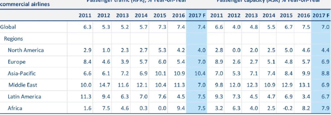
Aviation transported approximatively 3.8 billion passengers on commercial airlines in 2016, and this value is increasing with a rate higher than 7% in the last three years. Tab. 1.I reports the trend of the air passenger traffic [1].
Because most of the flights are between different countries, a key point for the success of the aircraft market is a proper coordination in terms of rules and standards.
The European air travel, for example, is actually responsible for an Air Traffic Management (ATM) of about 26,000 flights daily. In July 2017, the Network Manager has handled the record of one million flights across the EUROCONTROL network and in several occasions there were more than 35,000 flights in a single day [2]. In order to allow the sustainability of the future air transport in Europe, there are already new common rules and procedures (resulting by two
2
Single European Sky, SES, legislative packages) for the establishment of the aircraft safety, capacity and efficiency standards.
The aircraft industry is also taking into account the emissions related to the global warming and the climate changes, as it is happening in the automotive sector too. The Advisory Council for Aeronautics Research in Europe (ACARE) has set that by 2020 the air transportation should achieve a 50% reduction of Co2 emissions, 80% reduction of NOx emissions, 50% reduction of external noise and a green design, manufacturing, maintenance and disposal product life cycle [3].
In terms of economic impact, the fuel is still responsible of about 18% of the operating costs, for a total fuel cost of about US$130 billion every year. As can be seen in Tab. 1.II [4], the impact of the fuel cost is definitely important. Furthermore, the political and economic choices of the different countries of the world significantly affect the cost of the fuel of the total cost for the customers [5]. It results that many efforts aim to increase even more the efficiency of the propulsive and auxiliary systems.
Tab. 1.I – IATA: Statistic on commercial airline.
Multiphase Machines for More Electric Aircraft applications
3
For the longer-term future aircrafts, it is estimated that the development of hybrid-electric and battery-powered aircrafts could contribute to meet the industry goal of reducing aviation’s global carbon footprint by 50% by 2050, compared to 2005. Indeed, the actual technology is already mature, and huge efforts will not result in equivalent improvements, while the aircraft electrification process seems to be a good possible solution. A study from Munich-based think tank Bauhaus Luftfahrt (“Ce-Liner”) finds that larger electrically powered commercial aircraft could be possible from around 2035, and could cover routes of up to 1600 km in the subsequent years, assuming continuing strong progress in battery technology [6]. Of course, the increase of the electrical power on-board makes the efficiency and reliability of the electrical grid, the power generators and the drives a central point in the research for the future technologies. That is why there is such a spread of projects related to the More Electric Aircraft (MEA), More Electric Engine (MEE) and All Electric Aircraft (AEA) applications in the universities and companies around the world. In terms of European research, the most important programme is Clean Sky, where the collaboration between industries and universities is resulting in new idea and a series of demonstrators that aim to reduce the “emission and noise footprints of the aircraft with new engine architectures, improved wing aerodynamics, tighter composite structures, smarter trajectories, and more electrical on-board energy” [7].
The idea of More Electric Aircraft
The aerospace industry challenges are similar to the automotive industry ones in terms of emissions, fuel economy and costs. As in the automotive market, the aerospace trend is to move toward the increasing use of More Electric drives.
The MEA concept provides for the utilization of electric power for all the non-propulsive systems of an aircraft. The traditional systems are also driven by hydraulic, pneumatic and mechanical sources. These non-electrical systems need a heavy and bulky infrastructure for the
4
power transmission, and the difficulties on the diagnosis and localization of the faults limit their availability. Fig. 1.1 [3] shows a standard power flow in a civil aircraft.
Instead, in a MEA design, the jet engine completely provides the aircraft trust, and an embedded generator provides the power required by all the electrical loads, as shown in Fig. 1.2 [3]. The Airbus Boeing 787 Dreamliner is an example that represents the recent industrial development of the MEA technology, and similar developments can be found on the other MEAs.
Boeing 787 Dreamliner was designed to be the first airliner with the use of composite as the primary material of its airframe and to move toward the idea of MEA, with the aim of increasing the efficiency of about 20% [8]. The advancements in engine technology, provided by GE and Rolls-Royce, are the biggest contributor to the airplane’s overall full efficiency improvements [9]. To meet the requirements in terms of efficiency, reliability, availability, lightness and costs, one of the most important improvement on the design is that it includes mostly electrical flight systems, with a bleed-less architecture that allows extracting more efficiently power from the propulsive system, by two generators on each engine, and electrical brakes (rather hydraulically actuated brakes). The total electrical power (1 MVA) is subdivided in two 500 kVA channels, and two on the Auxiliary Power Units (APU), increasing the efficiency of the propulsion system. What has traditionally powered by bleed-air from the engine has been transitioned to an electric architecture. In particular, the only left bleed system on the Boeing 787 is the anti-ice system for the engine inlets [10, 11].
Furthermore, the 787 can be started without any ground power. To start the engine, the APU battery system is used to power the engine generators that start the engines in motoring mode [11]. Of course, owing to the starting profile, together with the emergency load profile, the sizing and the selection of the batteries have to be redesigned in MEA to meet the new power requirements, increasing the complexity of the new generation aircrafts [12].
Multiphase Machines for More Electric Aircraft applications
5
Because of the essential reliability of the total system, moving to an electrification of the aircraft needs to introduce redundancies in the electrical system, and the final layout is as the one shown in Fig. 1.3 [11]. As example of this redundancy, Boeing 787 has demonstrated that it can fly for more than six hours with only one of the two engine (indeed it is a twin-engine aircraft) and one of the six generators working [13].
The no-bleed architecture of the Boeing 787 affects also its electrical systems, where a new 230 V ac at 360-800 Hz and ± 270 V dc voltage lines are added to the traditional 115 V ac at 400 Hz and 28 V dc. The ± 270 V dc voltage is reached by auto-transformer-rectifiers.
Gearboxes connect the generators to the engine, working at a variable frequency (360-800 Hz) proportional to the engine speed. This allows avoiding the constant speed drive of the Integrated Drive Generator (IDG), which is the most complex component. As a result, the IDG reliability increases using an easier and cheaper technology.
The Boeing 787 is a study example that shows the actual available technology for civil aircrafts and represents the efforts needed to introduce the MEA technology on-board.
The idea of More Electric Engine
The aviation industry has always pushed the boundaries of technology in order to create quieter and more efficient aircrafts, and even before the first light of the More Electric Boeing 787 Dreamliner, the main companies (as GE and Rolls-Royce) were looking on developing the next aircraft technology: the More Electric Engine. The idea of MEE is to replace all the accessories mechanically driven by the engine (oil, fuel and hydraulic pumps and the generators) with electrically driven ones, and produce the needed electrical power by embedded generators
6
directly attached on the engine shaft, rather than connect them by means of a mechanical gearbox [14, 15]. Furthermore, one of the key features needed to realize a MEA technology, is that the electrical generator can start the engine and can provide the electrical power to the loads with enough efficiency and reliability. Indeed, all the non-propulsive power comes from these embedded generators, and they must reach a level of availability and maturity that ensures a neglectable risk of failure for the system.
The MEE requirements need new architectures and technologies of electrical machines and drives. There are criticalities of having a high power and high power density electrical machine embedded on the shaft of the propulsive system that satisfies the requested reliability [16]. In particular, the machine might rotate at high speed (up to 10-50 krpm) in a harsh environment with high temperatures and vibrations. Furthermore, there are space and assembly limitations. That is why the research is focusing so much on the development of MEE solutions.
Fig. 1.4 [17] shows an example of embedded starter/generator.
To design a MEE it is essential to choose where to locate the starter/generators and the other generators, and the topology of the electrical machines.
Embedded starter/generator location
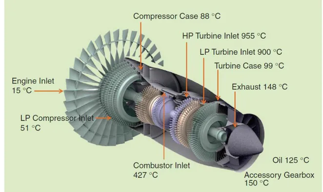
The generators could be placed on the Low Pressure shaft (LP) or on the High Pressure Shaft (HP) of the turbine engine. As can be seen form Fig. 1.5 [17], the two locations make the machine work at different pressures, temperatures and rotational speeds.
The rotational speed affects the size of the generator once its output power is fixed. The generators on the LP shaft will have a lower power density than the generators on the HP shaft (rotating at about 10000-20000 rpm). The temperature is lower on the LP side, since the HP
Multiphase Machines for More Electric Aircraft applications
7
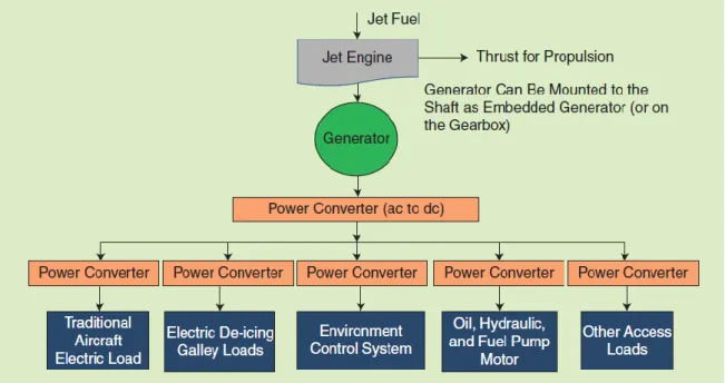
generator would be near the exhausted air outlet (with an ambient operating temperature around 300-400 ºC), but the lower pressure reduces the natural thermal cooling of the generator [18]. A typical MEE layout is shown in Fig. 1.6 [17]. As the starter/generator is placed on the HP shaft, it is one of the most stressed drives, because of the high temperature environment [19].
Embedded starter/generator machine topologies
According to [14], the main electrical machine topologies used for starter/generator application are:
Switched Reluctance Machine (SRM)
Permanent Magnet Brushless Machine (PMBM)
Induction Machine (IM)
The main advantage of SRM is their robustness, reliability and availability in a harsh environment, owing to the absence of permanent magnets and windings on the rotor. However, its airgap must be larger than the other topologies in order to reduce the torque pulsations and acoustic noise produced by its double saliency. Furthermore, in high seep applications the fast pulsating fields might cause high rotor losses.
PMBM are preferred for their higher power density, torque density, power factor, efficiency and easy controllability when compared with SRM and IM. In case of fault, the PM machines are intrinsically less fault tolerant because of the presence of the induced back emf and the demagnetization issue [20].