N. 11 – JANUARY 2021
THE ESTIMATION RISK AND
THE IRB SUPERVISORY
FORMULA
by Simone Casellina, Simone Landini and
Mariacristina Uberti
The EBA Staff Papers Series describe research in progress by the author(s) and are published to elicit comments and to further debate. Any views expressed are solely those of the author(s) and so cannot be taken to represent those of the European Banking Authority (EBA) or to state EBA policy. Neither the EBA nor
ABSTRACT
In many standard derivation and presentations of risk measures like the Value-at-Risk or the Expected Shortfall, it is assumed that all the model’s parameters are known. In practice, however, the parameters must be estimated and this introduces an additional source of uncertainty that is usually not accounted for. The Prudential Regulators have formally raised the issue of errors stemming from the internal model estimation process in the context of credit risk, calling for margins of conservatism to cover possible underestimation in capital. Notwithstanding this requirement, to date, a solution shared by banks and regulators/supervisors has not yet been found. In our paper, we investigate the effect of the estimation error in the framework of the Asymptotic Single Risk Factor model that represents the baseline for the derivation of the credit risk measures under the IRB approach. We exploit Monte Carlo simulations to quantify the bias induced by the estimation error and we explore an approach to correct for this bias. Our approach involves only the estimation of the long run average probability of default and not the estimation of the asset correlation given that, in practice, banks are not allowed to modify this parameter. We study the stochastic characteristics of the probability of default estimator that can be derived from the Asymptotic Single Risk Factor framework and we show how to introduce a correction to control for the estimation error. Our approach does not require introducing in the Asymptotic Single Risk Factor model additional elements like the prior distributions or other parameters which, having to be estimated, would introduce another source of estimation error. This simple and easily implemented correction ensures that the probability of observing an exception (i.e. a default rate higher than the estimated quantile of the default rate distribution) is equal to the desired confidence level. We show a practical application of our approach relying on real data. (JEL C15, G21, G32)
KEYWORDS
1. Introduction
More than fifteen years ago, the Basel Committee on Banking Supervision (BCBS) renewed the prudential regulation for banks with the introduction of a risk-based framework (widely known as Basel II), and allowed financial institutions to use their internal models to calculate minimum capital requirements for major risk types1.
While for market and operational risks banks were endowed with higher flexibility for the definition of the models, as regarding the credit risk, the BCBS imposed a specific model, leaving to the banks the role of providing the estimate of some model parameters.
For credit risk, the BCBS relies on a stochastic credit portfolio model aimed at providing the estimate of the loss amount which will be exceeded with a predefined probability. This probability represents the likelihood that a bank will not be able to meet its own credit obligations by resorting to its capital. 100% minus this likelihood is the confidence level, indicated with 𝛼, that is arbitrarily set, and the corresponding loss threshold is called Value-at-Risk (𝑉𝑎𝑅) at this confidence level. The 𝑉𝑎𝑅 summarises the worst case loss over a target horizon that will not be exceeded with a given level of confidence (Jorion, 2007, pp.viii). Stated otherwise, 𝑉𝑎𝑅 is the 𝛼-quantile of the loss distribution. Therefore, for example, by setting the confidence level at 𝛼 = 99%, then 𝑉𝑎𝑅𝛼 evaluates
the largest loss exceeding 99% of all possible losses, or the extreme loss that is expected to be exceeded with a probability of 1%.
In general, to compute standard risk measures such as the 𝑉𝑎𝑅, or the Expected Shortfall, it is necessary to estimate some parameters and these estimates are subject to estimation uncertainty. Replacing the true parameters’ value in the theoretical formula with sample estimates, that are based on sampling observations, introduces an additional source of uncertainty, the estimation risk2. The BCBS recognises the problem of the estimation error. Usually, the standard3 confidence level for 𝑉𝑎𝑅 is set to 99% or 99.5% but in BCBS (2005) it is stated that the confidence level is set to 99.9%, and that this high confidence level was chosen also to protect against estimation errors that might inevitably occur from banks’ internal estimates.
To clarify this point, it is useful to introduce the following notation. Let 𝐿 be a continuous real-valued random variable whose outcomes are values of the portfolio loss. The set of all possible values 𝐿 may assume is here indicated with the short-hand notation {𝐿} ⊂ ℝ+, namely the realisations space of 𝐿. Being a random variable,
it is completely described by its CDF (cumulative distribution function), whatever it is. The CDF depends on the parameter 𝜃, more formally 𝐹𝐿(. ; 𝜃): {𝐿} → [0,1]. Therefore, ℙ(𝐿 ≤ 𝑥) = 𝐹𝐿(𝑥; 𝜃) is the probability that the
portfolio loss does not exceed the value 𝑥 ∈ {𝐿}. Assume now the confidence level 𝛼 has been somehow set. If 𝑙(𝛼; 𝜃) is the amount of loss that may be exceeded with a probability 𝛼 then 𝑙(𝛼; 𝜃) is the 𝑉𝑎𝑅 of 𝐿 at the confidence level 𝛼: that is 𝑙(𝛼; 𝜃) ≡ 𝑉𝑎𝑅𝛼𝜃({𝐿}), notice that the 𝑉𝑎𝑅 of 𝐿 is evaluated over the set of all possible
1 BCBS (2004), updated in 2005 and then revised in June 2006.
2 It is worth clarifying the meaning of true and estimated parameter notions. Of course, each bank owns almost exhaustive
information about its borrowers, so the bank does not really ‘estimate’ but ‘computes’ a parameter’s value. Nevertheless, Regulation reports on the true value of a parameter, as if it were understood like a super-population value: this is, the meaning of the ‘true value of a parameter’. Clearly, different banks own different portfolios and the portfolio of a bank is a population to the bank, therefore parameters’ values change from bank to bank as if each bank’s portfolio were a sample: such a super-population is unknown to single banks while it is assumed to be known by the Regulator. Differently said, although the Regulator does not really observe all the banks’ portfolios while each single bank truly observes its own one, the parameters’ values set by the Regulator are true in the sense stated above, actually meaning that they are reference or target values set with prudential aims that have a strong theoretical ground against a weak empirical counterpart. Therefore, ‘estimation risk’ means both that different banks may apply different estimation methods so obtaining different values of the same parameter, and even though two banks apply the same method, they obtain different values because they operate with different portfolios, that are samples of that super-population.
3 For example, Jorion (2007) states that 99% confidence level has become a standard choice in the industry. Nobody knows
what the empirical motivations of this choice are, but almost everyone is confident that this value may protect against extreme, as well as unexpected, loss events.
realisations {𝐿}. In other terms, 𝑉𝑎𝑅𝛼𝜃({𝐿}) is the 𝛼-quantile of 𝐹𝐿(. , 𝜃), that is ℙ (𝐿 ≤ 𝑉𝑎𝑅𝛼𝜃({𝐿})) =
𝐹𝐿(𝑉𝑎𝑅𝛼𝜃({𝐿}), 𝜃) = 𝛼 therefore ℙ (𝐿 > 𝑉𝑎𝑅
𝛼𝜃({𝐿})) = 1 − 𝛼. According with this modeling, also the 𝑉𝑎𝑅
depends on the parameter 𝜃. Let 𝜃̂ be an estimator of 𝜃 then 𝑙(𝛼; 𝜃̂) = 𝑉𝑎𝑅𝛼𝜃̂({𝐿}) is an estimator of 𝑉𝑎𝑅𝛼𝜃({𝐿}).
To simplify the notation, we write 𝑉𝑎𝑅𝛼= 𝑉𝑎𝑅𝛼𝜃({𝐿}) to indicate the 𝛼-quantile on the uncountable set {𝐿} that
represents the measure of risk and 𝑉𝑎𝑅̂ = 𝑉𝑎𝑅𝛼 𝛼𝜃̂({𝐿}) is the estimator of the quantity 𝑉𝑎𝑅𝛼.
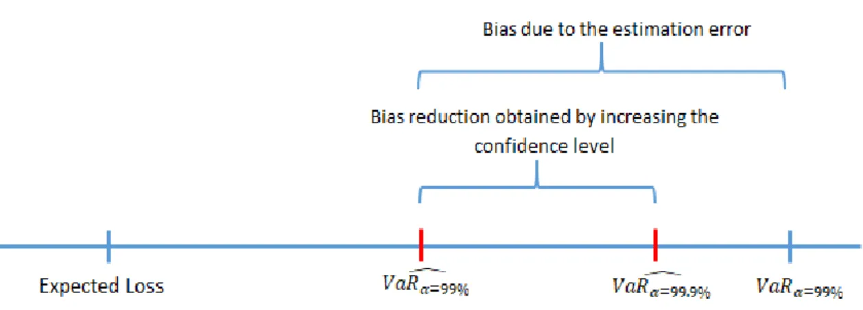
We now come back to the decision of the BCBS to set the confidence level 𝛼 to a higher than usual value both for prudential purposes and also to account for the additional-risk due to estimation error. For example, consider the target confidence level were 𝛼 = 99%. Due to the need to estimate the parameter 𝜃, one may suspect that the estimated 𝑉𝑎𝑅̂99% would not ensure that the realised loss exceeds this threshold with a probability 1% =
100% − 𝛼 as required. In other terms, it is possible that the probability of the loss exceeding 𝑉𝑎𝑅̂99% is higher than 1% or, equivalently, that 𝑉𝑎𝑅̂99% may be a downward biased estimator of 𝑉𝑎𝑅99%. By increasing the level
of confidence (𝛼), for instance up to 99.9%, the estimated value of the 𝑉𝑎𝑅 increases and this can reduce, or completely offset, the bias. Figure 1 describes this situation: it is worth mentioning that the 𝑉𝑎𝑅̂99.9% could also exceed the true value 𝑉𝑎𝑅99%. Notice that 𝑉𝑎𝑅99% is the theoretical Value-at-Risk for the bank’s portfolio at
99% confidence while 𝑉𝑎𝑅̂99% is the estimated value.
Figure 1 .: Comparison between the “true” and the estimated VaR.
Despite the BCBS declaration to set a higher than usual confidence level , also with the explicit aim to account for the estimation error, the European Regulation requires banks adopting the internal models to add a further Margin of Conservativism (MoC) that should somehow be proportional to the estimation error. In detail, pursuant to Article 179 (1) (f) of EU Regulation 575/2013 (the CRR, see EU (2013)): […] an institution shall add to its estimates a margin of conservatism that is related to the expected range of estimation errors. Where methods and data are considered to be less satisfactory, the expected range of errors is larger, the margin of conservatism shall be larger.
Furthermore, EBA (2017) states that the quantification of the MoC for the general estimation error should reflect the dispersion of the distribution of the statistical estimator. This requirement may have two interpretations. The first one is that the correction introduced by the BCBS, i.e. setting the confidence level at 99.9%, is deemed insufficient. The second one is that at European level it has been decided that the target confidence level is 99.9% instead of 99%. Following the first interpretation, i.e. the desired confidence level is lower than 99.9% (like 99% or 99.5%) but a higher level is needed to account for the estimation error, this paper aims at testing if setting the confidence level at 99.9% is sufficient to offset the estimation error that would be accounted with a confidence level of 99% or 99.5%. Under the second interpretation, where the targeted confidence level is indeed 99.9%, we analyse a possible approach to introduce an MoC to account for the estimation error. With these aims, we first introduce the estimation error of the 𝑃𝐷 parameter (probability of default) in the Asymptotic Single Risk Factor model (ASRF) that is the standard theoretical framework adopted by the BCBS. In
many of the standard presentations of this framework, it is assumed that the parameters of the model are known, while in practice they must be estimated. Moreover, a major contribution of this paper is to derive the stochastic characteristics of the 𝑃𝐷 estimator from the same hypothesis underlying the ASRF model. Finally, through Monte Carlo (MC) simulations, we derive the magnitude of the estimation error in connection with different levels of 𝑃𝐷 and of other parameters, namely the asset correlation (𝜔), the confidence level (𝛼) discussed above and the number of default rates observed i.e. the length of the time series available.
The rest of the paper is organised as follows. Section 2 reviews the literature; Section 3 describes the framework underlying the BCBS Supervisory Formula i.e. the Asymptotic Single Risk Factor model; Section 4 studies the stochastic characteristic of the default rates that can be derived from the ASRF and provides MC simulation results to assess the validity of the asymptotic results obtained; Section 5 introduces the estimation error in the framework and addresses the issue of adequacy of a confidence level equal to 99.9% to overcome the estimation error associated with a targeted confidence level of 99% or 99.5%; Section 6 deals with a possible approach to correct for the estimation error for a given confidence level; Section 7 provides an empirical application of the results obtained relying on real data; Section 8 concludes.
2. Literature review
Since the introduction of internal models in the supervisory framework, the Regulators have raised the issue of errors arising in the internal model estimation process, calling for margins of conservatism to cover possible underestimation in capital. The 2006 Basel Accord, International Convergence of Capital Measurement and Capital Standards (BCBS, 2006) in paragraph 451 states: In general, estimates of PDs, LGDs, and EADs are likely
to involve unpredictable errors. In order to avoid over-optimism, a bank must add to its estimates a margin of conservatism that is related to the likely range of errors. Where methods and data are less satisfactory and the likely range of errors is larger, the margin of conservatism must be larger. A similar statement can be found in
the CRR and in particular in Article 179. More recently, the EBA has devoted a material share of its 2017 Guidelines on model estimation - see EBA (2017) - to build up a framework to define, classify and quantify the Margin of Conservatism (MoC). In the context of the ECB targeted review of internal models (TRIM4) one of the items analysed has been the banks’ approaches to quantify the MoC. The ECB (2018) guide to internal models specifies that the MoC should be based on the distribution of the PD estimator, which is the average of one-year default rates across time, considering that the uncertainty is primarily driven by the statistical uncertainty of each one-year default rate and the length of the time series.
Notwithstanding this requirement, a solution shared by banks and regulators has not yet been found. In the BIS working paper 280, Tarashev (2009) explores the issue of parameter uncertainty under the Asymptotic Single Risk Factor (ASRF) model of portfolio credit risk by allowing for noisy estimates of both the probability of default (PD) and asset-return correlation. The approach suggested in this paper relies on the Bayesian approach. In turn, this implies that the model developer has to define a prior probability distribution for the parameters that must be estimated. The advantage of this approach is that it comes to define a closed form solution; the drawback is that it requires the definition of a prior distribution for the PD and the asset correlation.
Recently, in the AIFIRM (2019) position paper the problem of the introduction of an MoC in the IRB framework have been studied from a more practical and pragmatic point of view. The main strength of this paper is that it deals with all the three parameters (PD, LGD and EAD).
4 The TRIM is a large-scale project conducted by the ECB in close cooperation with the NCAs over 2016-2020. Its aim is to
reduce inconsistencies and unwarranted variability when banks use internal models to calculate their risk-weighted assets. The project combines detailed methodological work (the ECB Guide to internal models was published as a result of it) with the execution of about 200 on-site investigations.
More generically, references to the problem of estimation error in the quantification of risk measures can be found in a standard textbook about the VaR like Jorion (2006) (Chapter 5) and in some papers like Figlewski (2003) that examined the effect of estimation errors on the VaR by simulation. Christoffersen (2005) studied the loss of accuracy in the VaR and ES due to estimation error, and constructed bootstrap predictive confidence intervals for risk measures. Escanciano (2010) studied the effects of estimation risk on backtesting procedures. These studies showed how to correct the critical values in standard tests used to assess VaR models. Gourieroux (2012) proposed a method to directly adjust the VaR to estimation risk, by computing an Estimation adjusted VaR, denoted EVaR, ensuring the right conditional coverage probability at order 1/n.
As in Figlewski (2003), by means of Monte Carlo simulations, in this paper we primary demonstrate that, in the classic ASRF framework, the need to estimate the long run probability of default causes an underestimation of the true quantiles of the default rates distribution. In line with Tarashev (2009), our aim is to provide an approach to correct the estimated quantile of the default rates distribution to ensure that the probability of observing an exception is equal to the desired confidence level. However, a feature of our approach is that we develop our reasoning remaining coherent with the ASRF framework without the need to introduce further hypotheses or other elements such as the prior distributions or other parameters which, having to be estimated, would introduce another source of estimation error.
3. The ASRF theoretical framework
The aim of the next two sections is twofold. On one hand we present the ASRF theoretical framework underlying the Supervisory Formula i.e. the algorithm that, in compliance with the Regulation, provides the computation of the risk weight for credit assets under the Internal Rating Based Approach (IRB-A). On the other hand, we introduce the estimation error inside this framework to analyse its effect on the quantification of the risk measures. For the sake of simplicity, we disregard some aspects of the Supervisory Formula, such as the maturity adjustment, and we assume the asset correlation 𝜔 as a fixed parameter, while in the BCBS framework it varies as a function of probability of default, 𝑃𝐷5.
Credit risk has been traditionally interpreted as default risk, that is, the risk of loss from a borrower, or counterparty’s failure, that becomes unable to pay back the owed amount (principal or interest) to the bank on time. In other words, it is the risk of loss related to the non-performing loans (NPL) that are borrowers at-default, unable to respect the previously agreed payment schedule6. Among a wide stream of credit risk models (Crc,
2008), the BCBS adopted the Asymptotic Single Risk Factor (ASRF) model introduced by Gordy (2003). When a portfolio consists of a large number of relatively small exposures, idiosyncratic risks associated to individual exposures tend to cancel out one another and only systematic risks, that homogeneously affect all the exposures, have a material impact on portfolio losses. In the ASRF model, all systematic (or system-wide) risks, that affect all borrowers to a certain degree, like industry or regional risks, are modelled with only one systematic risk factor (BCBS, 2005).
Under the ASRF framework, it is possible to estimate both the expected (EL) and unexpected (UL) losses associated with each credit exposure. The expected loss is computed as a product of the probability of default (𝑃𝐷) and the loss given default (𝐿𝐺𝐷) parameters. It is worth mentioning that while the 𝑃𝐷 represents the expected default rate under normal business conditions (also named long run – LR – or through the cycle 𝑃𝐷),
5 For some asset classes, like residential mortgages and qualifying revolving exposures, the asset correlation is indeed set
equal to a constant.
6 A more comprehensive definition includes the risk of loss of value from a borrower migrating to a lower credit rating grade
without having defaulted. However, when considering traditional bank portfolios, mainly constituted by loans and advances to companies or families for which a market does not exist, only the traditional definition of credit risk matters, that is the “the default only” framework.
the 𝐿𝐺𝐷 is meant to representing a conservative value that can be expected to be observed in stressed (downturn – DWT) conditions7. The Expected Loss can be expressed as8:
𝐸𝐿 = 𝑃𝐷𝐿𝑅⋅ 𝐿𝐺𝐷𝐷𝑊𝑇 (1)
For each borrower, banks are required to estimate, the 𝑃𝐷𝐿𝑅 and the 𝐿𝐺𝐷𝐷𝑊𝑇 parameters.
The quantification of the Unexpected Loss (𝑈𝐿) is obtained by conditioning the 𝑃𝐷 to a conservative value of the single systematic risk factor. In practice, the aim of the Supervisory Formula is to transform the long run average 𝑃𝐷 in the stressed 𝑃𝐷 or the 𝑃𝐷 expected under downturn conditions:
𝑈𝐿 = 𝑃𝐷𝐷𝑊𝑇⋅ 𝐿𝐺𝐷𝐷𝑊𝑇− 𝐸𝐿 = (𝑃𝐷𝐷𝑊𝑇− 𝑃𝐷𝐿𝑅) ⋅ 𝐿𝐺𝐷𝐷𝑊𝑇 (2) The conditional 𝑃𝐷 is obtained as a function of the long run 𝑃𝐷, and the mapping is derived as an adaptation of Merton’s (1974) single asset model. Under this framework, it is possible to derive the entire distribution of the annual probability of default. For sufficiently large portfolios, the Law of Large Numbers holds so that deviations from the long run value are driven exclusively by the common systemic factor.
Figure 2 represents a possible series of observed default rates over a period of 15 years (data are fictitious): the probability distribution of the default rates is also represented. From a prudential standpoint, the quantity of interest is represented by the quantiles of this distribution that is also known as the Worst-Case Default Rate (WCDR). In the figure, the expected value of the distribution is equal to 5%, i.e. 𝑃𝐷 = 5%, and the 99%-quantile is about 𝑃𝐷 = 10%. This means that it can be expected that the realised default rate in a given year will be lower than 10% with 99% of probability or, symmetrically, that the default rate in a given year will exceed the value of 10% with probability 1%. Coherently with the notation introduced so far, {𝐷𝑅𝑡} represents the set of the
default rates, therefore 𝑉𝑎𝑅𝛼=99%𝑃𝐷=5%({𝐷𝑅𝑡}) = 10%9. In this simplified example, we consider the observed
highest default rate as the quantity of interest (WCDR).
Under the regulatory framework, it is assumed that the set of observations available to the bank is too limited to provide a reliable estimate of the WCDR and, for this reason, a model is developed to provide an estimate: this marks a further distinction between the true-theoretic and the estimated-empiric parameters introduced in the first section.
Figure 2 .: Annual default rates distribution and worst case default rate
7 During an economic downturn, losses on defaulted loans are likely to be higher than those under normal business
conditions. Average loss rates given default over a long period need to be adjusted upward to appropriately reflect adverse economic conditions.
8 This definition leads to a higher EL than would be implied by a statistical expected loss concept because the “downturn”
LGD will generally be higher than the average LGD. According to the Basel 2 guidelines, the EL is defined without the Exposure at Default (EAD) that is analysed separately with respect to EL and UL or, more simply, it is equivalent to consider a unitary EAD. Moreover, 𝐸𝐿 = 𝑃𝐷𝐿𝑅⋅ 𝐿𝐺𝐷𝐷𝑊𝑇 may be understood both as percent-EL or monetary-EL of a unitary exposition: in the following, when needed, the monetary-EL will be indicated as 𝐸𝐿€, in the same way 𝑈𝐿€ will be monetary-UL, otherwise UL is percent-UL.
9
Notice that the previously introduced 𝑉𝑎𝑅𝛼({𝐿}) is a monetary-quantity defined on all the possible loss values while 𝑉𝑎𝑅𝛼({𝐷𝑅𝑡}) is a percent-quantity defined over all the possible 𝑃𝐷 values.
We now introduce the ASRF framework, from which the Supervisory Formula is derived. The starting point of this construction can be considered the observation of a default rate in a given year for a given portfolio or sub-portfolio10. We can assume that this quantity represents an estimate of the true probability of default for that year. We must then recognise that the probability of default may vary year by year as a consequence of the external economic conditions. We can figure out these economic shocks as pushing the probability of default away from its equilibrium value at each year. This consideration allows for the possibility to consider that an ‘equilibrium’ or steady value for the probability of default exists and we define this value as the long run probability of default 𝑃𝐷𝐿𝑅. The term ‘long run’ is based on the idea that observing a sufficiently large number of default rates (i.e. with the availability of a long time series) and computing the average, it would be possible to obtain an estimate of the ‘equilibrium’ value11. We assume that the long run PD (𝑃𝐷𝐿𝑅) is known and we
derive an expression that enables us to quantify the quantiles of the distribution of the default rates for any given level of confidence. These quantiles are the worst case default rate (WCDR) estimated with a given level of confidence.
In the classical structural Merton-Vasicek model, the i-th creditworthiness change 𝑌𝑖,𝑡 is defined as a function of two random variables, namely the single systematic risk factor 𝑍𝑡, that homogenously spreads its effect on each
single borrower, and an idiosyncratic term 𝑊𝑖,𝑡, that heterogeneously hits the i-th borrower only. The hypotheses12 used are the following
HP. 1 𝑊𝑖,𝑡 ~𝑖𝑖𝑑 𝒩(0,1)
HP. 2 𝑍𝑡 ~ 𝒩(0,1)
HP. 3 𝐶𝑜𝑟𝑟(𝑊𝑖,𝑡 , 𝑍𝑡) = 0
HP. 4 𝐶𝑜𝑟𝑟(𝑍𝑡−1 , 𝑍𝑡) = 0
HP. 5 𝑌𝑖,𝑡 = 𝑌(𝑍𝑡, 𝑊𝑖,𝑡; 𝜔) is linear HP. 6 The portfolio is infinitely grained
(3)
10 In general, we are assuming we are dealing with a group of homogeneous clients in terms of credit worthiness.
11 In other terms, the 𝑃𝐷𝐿𝑅 is the probability of default that would occur if there were no correlation between the counterparties, or if there were the idiosyncratic risk factor only. As far as the systematic factor is not directly observable, assuming a 𝑃𝐷𝐿𝑅 modelling based on such a latent factor means that the value of the 𝑃𝐷𝐿𝑅 is not directly observable as well. However, as proved in the following, from the statistical point of view, the average of the default rates is an unbiased estimator of 𝑃𝐷𝐿𝑅.
12
From a formal-theoretic point of view, hypotheses in (3) should be said axioms, indeed none of them have been ever neither validated or falsified on data: for a logic-formal distinction between the notions of axiom and hypothesis in economic and applied mathematics literature, as well as other notions that are involved in Section 4, see Landini et al. (2020) and references cited therein.
𝜔 ∈ (0,1) is an exogenous parameter set by the Regulator: portfolios of different instruments have their specific value of 𝜔, also named as the factor loading, that shapes the correlation of the systematic risk factor with the individual creditworthiness change. The HP. 4 is usually not mentioned in the standard presentations of the ASRF and, indeed, it is not necessary as long as only one period is mentioned. We included this hypothesis because, in the next section, we introduce the estimator of a parameter of the model as the average of 𝑡 = 1,2 … 𝑇 observations. So, for the sake of simplicity, HP.4 excludes any serial correlation: namely, time observations are serially independent13. According to the underlying hypotheses in (3) the model is specified as follows:
𝑌𝑖,𝑡 = 𝑌(𝑍𝑡, 𝑊𝑖,𝑡; 𝜔): = √𝜔 ⋅ 𝑍𝑡+ √1 − 𝜔 ⋅ 𝑊𝑖,𝑡 ~ 𝒩(0,1) (4) therefore, 𝑌𝑖,𝑡 is a standard normal random variable. Note that, as long as the systematic term homogeneously
spreads its effects across heterogeneous borrowers, the model considers that the borrowers in a given portfolio of the same bank are interrelated. The common risk factor 𝑍𝑡 represents the state of the economy. It might be helpful considering 𝑍𝑡 as the GDP annual growth rate: in this case, 𝑍𝑡< 0 would mean that a reduction of GDP
has been observed. However, one must bear in mind that the model assumes 𝑍𝑡 is a serially independent
standard normal random variable and that the linkage with the reality is obtained through the calibration or estimation of the two parameters of the model, namely 𝜔 and 𝑃𝐷𝐿𝑅: in this paper we take 𝜔 as given and focus our attention on 𝑃𝐷𝐿𝑅 only.
Assume 𝐷𝑖,𝑡 is a dichotomous variable with value 1 when 𝑌𝑖,𝑡< 𝑠 and 0 when 𝑌𝑖,𝑡≥ 𝑠: 𝑠 is here understood as a somehow known threshold. 𝐷𝑖,𝑡 represents the credit status of the i-th borrower as a probabilistic event, more
precisely: 𝐷𝑖,𝑡= 1 is associated to a default event (the borrower is at-default), 𝐷𝑖,𝑡= 0 is associated to a
performing state, whatever its rating grade is. On the basis of model (4), namely 𝑌𝑖,𝑡~ 𝒩(0,1), the credit state
probability of a borrower is:
ℙ(𝐷𝑖,𝑡; 𝑠) = {𝑃𝐷𝑖,𝑡 ≔ ℙ(𝑌𝑖,𝑡 < 𝑠) = Φ(𝑠) 𝑃(𝑌𝑖,𝑡 ≥ 𝑠) = 1 − 𝑃𝐷𝑖,𝑡
(5) The probability of default in a given period 𝑡 is different from the long run 𝑃𝐷 because it depends on the value realised by 𝑍𝑡 in that period. By conditioning to a given realisation 𝑍𝑡= 𝑧 it can be found that (4) becomes:
𝑌𝑖,𝑡𝑧 ~ 𝑁(√𝜔 ⋅ 𝑧 ,1 − 𝜔) (6)
More precisely, conditioning to a given realisation among the uncountable ones of the systematic term means that one assumes the possibility of fixing a precise given value of 𝑍𝑡, namely 𝑧, that may be either a negative or
positive real number: in the first case one considers an adverse systematic shock due to contingent cyclical effects somehow determined, in the second case one considers a positive cycle impact on individual creditworthiness. Therefore, the probability of default conditioned to 𝑍𝑡= 𝑧 is:
𝑃𝐷𝑖,𝑡𝑧 = ℙ(𝐷𝑖,𝑡 = 1|𝑍𝑡 = 𝑧; 𝑧 < 0) = ℙ(𝑌𝑖,𝑡𝑧 < 𝑠) = Φ (𝑠 − √𝜔 ⋅ 𝑧
√1 − 𝜔 ) = 𝑓(𝑧; 𝜔, 𝑠)
(7)
With this expression the conditional 𝑃𝐷 is defined as a function of the long run (unconditional) 𝑃𝐷, used to evaluate the quantity 𝑠 = Φ−1(𝑃𝐷𝐿𝑅), and the value 𝑧 assumed by the random variable 𝑍
𝑡, while the parameter
𝜔 is fixed by the Regulation. The Regulation is essentially interested in adverse shocks, 𝑍𝑡< 0. In this case, the
conditional 𝑃𝐷 is the stressed PD, a 𝑃𝐷 influenced by a downturn of the cycle. Therefore, the stressed 𝑃𝐷 is obtained through (7) by fixing 𝑍𝑡 to a non-positive percentile of the standard normal distribution:
13
We are aware this is a hard simplification that moves the modelling away from reality. Nevertheless this simplification will now affect the results within the ASRF theoretical framework. We leave this topic for further developments.
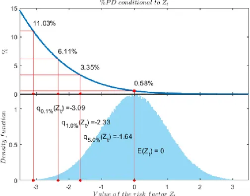
Figure 3 may help to understand the functioning of this mapping.
The figure is obtained by setting 𝜔 = 0.15, that is the regulatory value used for residential mortgages portfolios (Article 154 CRR). Let us develop few steps to apply (7). First of all, assume the long run 𝑃𝐷 is known and set at 𝑃𝐷𝐿𝑅= 1% such that 𝑠 = Φ−1(1%) ≅ −2.33. The BCBS sets the confidence level to 𝛼 = 99.9%, that is
equivalent to setting 𝑍𝑡 at 𝑧 = Φ−1(1 − 𝛼) ≅ −3.09. With this value for the systematic risk factor, by means of
(7) the value of the stressed 𝑃𝐷 is 𝑃𝐷𝑖,𝑡𝑧 = 11.03%. Notice that in this case, the stressed PD is more than 10
times the assumed long run value 𝑃𝐷𝐿𝑅. In this case, the bank would be asked to hold a level of own capital
sufficient to absorb the losses caused by any default rate up to about 11%.
Figure 3.: Conditional probability of default and systemic risk factor distribution with 𝑃𝐷𝐿𝑅= 1% and 𝜔 = 15%
In summary, we have seen that the conditional 𝑃𝐷 (7) depends on a given realisation 𝑧 of the standard normal systematic risk factor 𝑍𝑡 that homogeneously spreads its effect across borrowers, so they are somehow
interrelated by construction. Moreover, (7) explains that the conditional 𝑃𝐷 parametrically depends on the long run 𝑃𝐷 – indeed 𝑠 = Φ−1(𝑃𝐷𝐿𝑅) – and on the loading parameter 𝜔 that represents the correlation between
individual creditworthiness change and the systematic risk factor. Therefore, for a given 𝑃𝐷𝐿𝑅 and a fixed
credit-line-specific loading 𝜔, the conditional 𝑃𝐷 can be seen as a function of 𝑍𝑡= 𝑧, with a simplified notation 𝑃𝐷𝑖,𝑡𝑧 =
ℙ(𝐷𝑖,𝑡= 1|𝑍𝑡= 𝑧) = 𝑓(𝑧). Up to this point, we followed the standard presentation of the ASRF where it is
assumed all the relevant parameters are known. However, in the real-world practice, the bank estimates the long run 𝑃𝐷 as the empiric time-average of the observed default rates of the portfolio14. This implies that the
14
This is why the long run 𝑃𝐷 is commonly known as the long run average 𝑃𝐷, conveniently indicated as 𝑃𝐷𝐿𝑅𝐴. As long as the long run 𝑃𝐷 is an unknown parameter, we preferred not to indicate it as 𝑃𝐷𝐿𝑅𝐴 because the expression ‘long run average’ may suggest that it is an estimate while, from the theoretical point of view of the modelling, it is only a parameter that is to be estimated by the bank.
parameter 𝑃𝐷𝐿𝑅 is substituted with an estimator that, in turn, is a random variable and this implies an additional
source of variation15.
4. From theory to practice: the notion
of default rate
In the previous section, the ASRF theoretical framework has been discussed. The main issue to be clarified is now that the parameter long run 𝑃𝐷 is a theoretic notion and, in practice, nobody truly observes the 𝑃𝐷𝐿𝑅. Therefore,
the ASRF framework involves the theoretic notion of 𝑃𝐷 while it remains as a parameter to be estimated, and this aspect introduces the estimation risk issue. From a different point of view, it can be said that the results of the previous section succeed in matching with logical consistency with the restricted set of hypotheses in (3) and (4), indeed (7) follows without contradiction, but they fail to match with logical correctness because, as long as no objective measure of 𝑃𝐷 exists, they cannot be compared to a real-world outcome or, in the jargon of logic, they cannot be falsified. In practice, what the bank truly observes are default events after they realised.
As far as the bank only observes default events, the best the bank can do is to evaluate (i.e. compute) the default
rate (𝐷𝑅 from here onward) and use it as if it were the most objective measure of the conditioned 𝑃𝐷, i.e. the
𝑃𝐷 associated with a given realisation of the external factor. The bank evaluates the 𝐷𝑅 at time 𝑡 as the number of expositions found at default divided by the number of all the expositions in the portfolio. Then, having at hand a time series of default rates, it is possible to consider the average of these default rates as the estimator of the parameter 𝑃𝐷𝐿𝑅. We now develop the stochastic characteristics of the default rate that can be derived from the
ASRF framework. We then exploit these characteristics to specify the properties of the estimator of the parameter 𝑃𝐷𝐿𝑅.
The conditional default rate. Consider the creditworthiness change conditioned to a fixed value 𝑍𝑡= 𝑧 at time
𝑡, namely 𝑌𝑖,𝑡𝑧, in (6). Define a dichotomous random variable 𝐷
𝑖,𝑡𝑧 such that 𝐷𝑖,𝑡𝑧 = 1 if 𝑌𝑖,𝑡𝑧 < 𝑠 and 𝐷𝑖,𝑡𝑧 = 0 if 𝑌𝑖,𝑡𝑧 ≥
𝑠. As far as 𝑃𝐷𝑖,𝑡𝑧 = 𝑓(𝑧) is the conditional 𝑃𝐷16, that depends on the fixed 𝑃𝐷𝐿𝑅 and 𝜔 by construction, then
𝐷𝑖,𝑡𝑧 ∼ 𝐵𝑒𝑟(𝑝) where 𝑝 = 𝑓(𝑧). Therefore, within the theoretical framework of the ASRF model, the quantity 𝐷𝑅𝑡𝑧= ∑𝑁𝑖=1𝐷𝑖,𝑡𝑧 /𝑁 , defined on a portfolio of 𝑁 borrowers, is a Binomial random variable with parameters 𝑝 =
𝑓(𝑧) and 𝑁. By relying on the asymptotic approximation of the Binomial distribution to the Normal one, the 𝐷𝑅 conditioned to a given value 𝑧 of the risk factor 𝑍𝑡 is:
𝐷𝑅𝑡𝑧 = 1 𝑁∑ 𝐷𝑖,𝑡 𝑧 𝑁 𝑖=1 ~ 𝒩 (𝑓(𝑧),𝑓(𝑧) ⋅ (1 − 𝑓(𝑧)) 𝑁 ) (8)
Notice that 𝔼(𝐷𝑅𝑡𝑧) = 𝑓(𝑧), so that the annual conditional default rate is an unbiased estimator of the
conditional probability of default at a given period 𝑡. Moreover, for sufficiently large portfolios (i.e. asymptotically) the random variable 𝐷𝑅𝑡𝑧 converges to a constant that is equal to 𝑓(𝑧): that is 𝑝𝑙𝑖𝑚𝑁→∞𝐷𝑅𝑡𝑧=
15 Once more, it is worth bearing in mind that the bank’s portfolio is a population to the bank, therefore empiric values are
those observed by truth but, with respect to the theoretical modelling, i.e. from the Regulator’s point of view, each portfolio is to be understood as a sample from a super-population, therefore empiric values are estimates of the true, i.e. theoretic, parameters involved.
16
𝑓(𝑧). Therefore, within the ASRF theoretical framework, the conditional 𝐷𝑅 is an unbiased and statistically consistent estimator of the conditional 𝑃𝐷17.
The ASRF model assumes that 𝑁 is sufficiently large to consider the variability due to the idiosyncratic factor as irrelevant. The expression (8) helps to better clarify this point. For a given value of the external factor, 𝑍𝑡= 𝑧,
the model envisages a fixed probability of default defined in (7). However, the observable default rate is a random variable with distribution in (8) and its variability depends on the idiosyncratic factor 𝑊𝑖,𝑡. As far as the
variance of the conditional default rate decreases with the number of borrowers in the portfolio then, for a sufficiently large 𝑁, the variance of 𝐷𝑅𝑡𝑧 almost vanishes or it is practically null18. In practice, the number of
borrowers is exogenously given and it is possible that the number is not large enough for the Law of Large Numbers to hold, as assumed by the AFRS theory.
The probability distribution of the default rates. The portfolio default rate varies for each value of the systemic
risk factor 𝑍𝑡: that is, as 𝑍𝑡 varies a series of default rates is generated. The expected value of this series can be
expressed as follows:
𝔼({𝐷𝑅𝑡}) = 𝔼[𝔼(𝐷𝑅𝑡|𝑍𝑡 )] = ∫ 𝑓(𝑧)𝜑(𝑧)d𝑢
∞ −∞
In this expression, the expected value of each conditioned default rate, 𝑓(𝑧), is weighted by the probability of observing the particular value 𝑧, namely 𝜑(𝑧), where 𝜑(. ) is the standard normal PDF (probability density function). Therefore, 𝔼(𝐷𝑅𝑡) is the average of all the conditional default rates generated over all possible
realisations of the systematic risk term, as if 𝑍𝑡 were free to assume any feasible value. Bluhm et al. (2010,
Proposition 2.5.9) prove the expected value of the default rates is:
𝔼({𝐷𝑅𝑡}) = 𝑃𝐷𝐿𝑅 (9)
This expression enables us to better understand the role of the parameter 𝑃𝐷𝐿𝑅: if we had a long enough time series to be able to consider the realisation of all the possible scenarios together with the corresponding default rates, then it would be possible to obtain the parameter 𝑃𝐷𝐿𝑅 as the average of such default rates. Unfortunately, this is impossible in practice because the set of all possible default rates is neither finite nor countable, indeed the set of all possible values of 𝑍𝑡 is non-finite and uncountable as well. Bluhm et al. (2010)
also prove that the variance of the conditional default rates is:
𝕍({𝐷𝑅𝑡}) =Φ2[𝑠, 𝑠; 𝜔] − (𝑃𝐷𝐿𝑅)2= 𝜎
𝐷𝑅2 (10)
where Φ2[𝑠, 𝑠; 𝜔] is the bivariate Standard Normal CDF evaluated at (𝑠, 𝑠) while parametrically depending on
the loading factor parameter 𝜔. For example, Bluhm et al. (2010; Proposition 2.5.8) prove that the generic 𝛼-quantile of the unconditional distribution of 𝐷𝑅𝑡, 𝑞𝛼({𝐷𝑅𝑡}) ≡ 𝑉𝑎𝑅𝛼𝑃𝐷
𝐿𝑅
({𝐷𝑅𝑡}), is related to the (1 −
𝛼)-quantile of the systematic risk factor 𝑍𝑡, 𝑞1−𝛼({𝑍𝑡}) = Φ−1(1 − 𝛼), by means of the following expression:
𝑞𝛼({𝐷𝑅𝑡}) = Φ (Φ −1(𝑃𝐷𝐿𝑅) − √𝜔 ⋅ 𝑞 1−𝛼({𝑍𝑡}) √1 − 𝜔 ) = Φ ( 𝑠 − √𝜔 ⋅ Φ−1(1 − 𝛼) √1 − 𝜔 ) (11)
17 As a matter of fact, if one assumes the systematic risk factor 𝑍
𝑡 exists, although unobservable latent, then what happens at a given time 𝑡 is assumed being irremediably conditioned by the realisation 𝑍𝑡= 𝑧, whatever it is. One does not need to know 𝑍𝑡= 𝑧 by truth, one only needs to believe that (4) and (6) describe the world as it is.
This expression represents the bulk of the Supervisory Formula (Article 153 and 154 CRR). It is by means of this expression that one can evaluate the WCDR (worst-case-default-rate), the maximum default rate that can be observed with a given level of confidence.
5. The estimation error in the ASRF
framework
We now introduce the estimation error issue within the ASRF theoretical framework. We have seen that, if 𝑁 is sufficiently large, it is possible to predict any quantile of the distribution of the default rate by means of expression (11). However, this is true only if the parameter 𝑃𝐷𝐿𝑅 is known but, in practice, banks estimate it on
observed default rates. A natural candidate for the estimation of 𝑃𝐷𝐿𝑅 is the average of the observed default
rates: 𝐷𝑅 ̅̅̅̅ =1 𝑇∑ 𝐷𝑅𝑡 𝑇 𝑡=1 (12)
By means of (9) we know that the average of the default rates observed over 𝑇 periods is an unbiased estimator of the long run average 𝑃𝐷, therefore 𝔼(𝐷𝑅̅̅̅̅) =𝑃𝐷𝐿𝑅 should hold. Moreover, due to HP 4 in (3), the default
rates are serially uncorrelated19. By means of (10) we can also derive the variance of the estimator 𝐷𝑅̅̅̅̅, that is:
𝕍(𝐷𝑅̅̅̅̅) =Φ2[𝑠, 𝑠; 𝜔] − (𝑃𝐷 𝐿𝑅)2 𝑇 = 𝜎𝐷𝑅2 𝑇 (13)
It is worth noticing that the variance of the average default rate does not depend (at least asymptotically) on the portfolio size 𝑁 but only on the number of periods 𝑇. A common mistake is to think that the variance of the average default rate is equal to 𝑃𝐷𝐿𝑅⋅ (1 − 𝑃𝐷𝐿𝑅)/𝑇. This would be true only if 𝜔 were null. Two other mistakes
one may face are to estimate the variance of 𝐷𝑅̅̅̅̅ also as 𝑃𝐷𝐿𝑅(1 − 𝑃𝐷𝐿𝑅)/𝑁 or 𝑃𝐷𝐿𝑅(1 − 𝑃𝐷𝐿𝑅)/(𝑁 ⋅ 𝑇). As
long as we remain within the ASRF framework, both expressions are irredeemably wrong because they do not account for the fact that the idiosyncratic components 𝑊𝑖,𝑡 cancel out and the only source of variability is the
common systemic risk factor. Indeed, to obtain the (11) it is assumed that 𝑁 is sufficiently large to consider the variability stemming from the idiosyncratic factor as irrelevant. What remains is the variability of the default rates induced by the common factor. It is also important to mention that the expression (13) relies on the assumption HP.4, i.e. the external factor is serially uncorrelated. This is a hypothesis typically not confirmed by the data. With serially correlated default rates, the variance of the estimator would be higher. This aspect is relevant also because a possibility for the computation of the average default rate is to employ overlapping windows so that more than 1 default rate is computed for each year. In this way, the number of observations 𝑇 are increased but also the autocorrelation is likely to increase, so that it is possible that the estimated variance increases. We do not deal in this paper with the case of serially correlated default rates but this is a relevant aspect for future studies. Now that we have defined the estimator (12) of the parameter 𝑃𝐷𝐿𝑅, we can study the
quantity 𝑞̂({𝐷𝑅𝛼 𝑡})20, that is the estimator of the quantile of the distribution of the default rates:
19
If according to hypothesis HP.4 𝐶𝑜𝑟𝑟(𝑍𝑡−1 , 𝑍𝑡) = 0 then the default rates are serially uncorrelated.
20
To clarify the notation, as explained in Section 1, it must be said that 𝑞𝛼({𝑋}) is the theoretic 𝛼-quantile of the distribution of the quantity random variable 𝑋. Accordingly, 𝑞̂({𝑋}) is the estimator of the theoretic quantile of the same quantity. 𝛼
𝑞̂({𝐷𝑅𝛼 𝑡}) = Φ (Φ
−1(𝐷𝑅̅̅̅̅) − √𝜔 ⋅ 𝑞
1−𝛼({𝑍𝑡})
√1 − 𝜔 )
(14)
The main difference between (11) and (14) is that 𝑠 = Φ−1(𝑃𝐷𝐿𝑅), where the unknown parameter 𝑃𝐷𝐿𝑅
appears, has been substituted with Φ−1(𝐷𝑅̅̅̅̅), where the quantity 𝐷𝑅̅̅̅̅ has been involved as it can empirically be
obtained. It is also worth noticing that (11) represents a constant while (14) defines a random variable due to the variability of 𝐷𝑅̅̅̅̅: indeed, (14) is the estimator of the (11).
To investigate whether setting the confidence level to 99.9% instead of 99% or 99.5% is sufficient to adjust for the estimation error, we consider that the highest value of 𝜔 envisaged by the BCBS regulation is 𝜔 = 0.24 and that the minimum number of years that banks are allowed to employ for the estimation of the 𝑃𝐷𝐿𝑅 is 𝑇 = 5.
We then test whether setting the confidence level to 99.9% instead of 99% or 99.5% is sufficient to adjust for the estimation error in a situation where 𝜔 = 0.30, i.e. above the maximum value provided by the Regulation, and 𝑇 = 5, the minimum length for the estimation period that banks are allowed to use21. The experiment deals
with four values for the 𝑃𝐷𝐿𝑅, namely 0.1%, 1%, 5% and 10%.
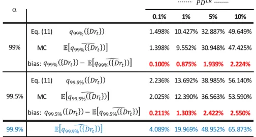
Table 1 reports the results obtained with 𝐵 = 2,000,000 Monte Carlo replicates. Results allow quantifying the effect of the estimation error comparing the value of the “true” 𝛼-quantile, obtained by means of the (11), and the expected value of the estimator defined by the (14), where the expected value has been obtained empirically by averaging the 𝐵 Monte Carlo replicates. It is possible to observe that (14) provides a downward bias of the 𝛼-quantile. For example, with 𝑃𝐷𝐿𝑅=0.1% and a confidence level of 99% we see that the WCDR (or the 𝑉𝑎𝑅) is 1.49% while the expected value of the estimator is 1.39%. It is also possible to conclude that, although the need to estimate the parameter 𝑃𝐷𝐿𝑅 causes a material downward bias in the estimator of the quantile of the
distribution of {𝐷𝑅𝑡}, by increasing the confidence level it is possible to offset this bias. In other terms, if the
target confidence were 99%, it is true that 𝔼(𝑞̂({𝐷𝑅99% 𝑡})) < 𝑞99%({𝐷𝑅𝑡}) but 𝔼(𝑞̂ ({𝐷𝑅99.9% 𝑡})) >
𝑞99%({𝐷𝑅𝑡}). Also considering a confidence equal to 99.5%, it is possible to observe that the estimator
𝑞̂ ({𝐷𝑅99.9% 𝑡} provides a prudential estimate that is able to completely offset the bias induced by the estimation error, in brief: 𝔼(𝑞̂ ({𝐷𝑅99.9% 𝑡})) > 𝑞99.5%({𝐷𝑅𝑡}).
Table 1.: 𝛼-quantiles of 𝐷𝑅𝑡. Analytic values of (11) vs empiric values of (14): confidence level at 99% and
99.9%, with 𝜔 = 0.3, 𝑇 = 5 and 𝑁 = 5,000
Notice that the difference between 𝔼(𝑞̂ ({𝐷𝑅99.9% 𝑡})) and 𝑞99%({𝐷𝑅𝑡}) appears definitely larger than the bias.
For example, with 𝑃𝐷𝐿𝑅= 1% the stressed 𝑃𝐷, i.e. 𝑞
99%({𝐷𝑅𝑡}), is 10.427%. The expected value of the
21 The variance of the estimator increases by increasing 𝜔 and reducing 𝑇. We then study the impact of the estimation risk
in a setting where the variability of the estimator is at its maximum.
0.1% 1% 5% 10% Eq. (11) 1.498% 10.427% 32.887% 49.649% MC 1.398% 9.552% 30.948% 47.425% 0.100% 0.875% 1.939% 2.224% Eq. (11) 2.236% 13.692% 38.985% 56.140% MC 2.025% 12.390% 36.563% 53.590% 0.211% 1.303% 2.422% 2.550% 99.9% 4.089% 19.969% 48.952% 65.873% bias: bias: 99% 99.5% a 𝑃𝐷 𝐿𝑅 𝑞99% 𝐷𝑟𝑡 𝔼 𝑞99%̂𝐷𝑟𝑡 𝑞99.5% 𝐷𝑟𝑡 𝔼 𝑞99.5%̂𝐷𝑟𝑡 𝔼 𝑞99.9%̂𝐷𝑟𝑡 𝑞99% 𝐷𝑟𝑡 − 𝔼 𝑞99%̂𝐷𝑟𝑡 𝑞99.5% 𝐷𝑟𝑡 − 𝔼 𝑞99.5%̂𝐷𝑟𝑡
estimator 𝑞̂({𝐷𝑅99% 𝑡}) is 9.552% so that the bias is equal to 0.875%. However, the expected value of
𝑞̂ ({𝐷𝑅99.9% 𝑡}) is 19.969%, so the Margin of Conservativism, 𝑀𝑜𝐶 = 𝔼[𝑞̂ ({𝐷𝑅99.9% 𝑡})] − 𝔼[𝑞̂ ({𝐷𝑅99% 𝑡})], is 10.42%, about ten times the absolute bias. In the Annex there is a graphical representation of the comparison between 𝑞99%({𝐷𝑅𝑡}) and the estimators 𝑞̂ ({𝐷𝑅99% 𝑡}) and 𝑞̂ ({𝐷𝑅99.9% 𝑡}).
6. A correction for the estimation error
in the ASRF framework
In the previous section, it has been proved that if the target confidence level were 99% then using 𝑞̂ ({𝐷𝑅99.9% 𝑡})
would be enough to get rid of the bias introduced by the estimation error, and this appears in accord with the BCBS perspective. However, it should be noticed that the banks cannot modify the level of confidence because it is set by the Regulator. Therefore, we now explore how a bank could introduce a Margin of Conservativism to control for the estimation error given the confidence level.
The approach we explore is obtained by substituting the estimator 𝐷𝑅̅̅̅̅ of 𝑃𝐷𝐿𝑅 with the upper bound of a
confidence interval estimator with confidence level 𝛽 ∈ (0,1). By means of (12) and (13) and for sufficiently large 𝑇 it is possible to refer to the Central Limit Theorem to conclude that:
𝐷𝑅
̅̅̅̅ ~ 𝒩 (𝑃𝐷𝐿𝑅 ; 𝜎𝐷𝑅
2 𝑇 )
(15)
This last result can in turn be used to specify a confidence interval around 𝐷𝑅̅̅̅̅. Let 𝛽 ∈ (0,1) represent the confidence level, then the upper bound of the confidence interval is:
𝑞𝛽({𝐷𝑅̅̅̅̅}) = 𝐷𝑅̅̅̅̅ + Φ−1(𝛽) ⋅ √𝜎𝐷𝑅 2
𝑇
(16)
Expression (16) is built so to ensure that the true value of the parameter 𝑃𝐷𝐿𝑅 does not exceed the value obtained with a given confidence level, i.e.:
ℙ (𝑃𝐷𝐿𝑅 < 𝐷𝑅̅̅̅̅ + Φ−1(𝛽) ⋅ √𝜎𝐷𝑅2
𝑇 ) = 𝛽
(17)
At this stage, it is important to pay attention to differences between the (14) and (16). Both expressions represent a quantile of the distribution of a random variable. (14) is applied to the default rates while (16) is applied to the estimator of the 𝑃𝐷𝐿𝑅. Moreover, (14) is interpreted as a risk measure, i.e. the 𝑉𝑎𝑅 at a given confidence level, while (16) is the upper bound of an interval estimator of a given parameter. We can now define a new estimator of the quantity (11), where the average of the default rate 𝐷𝑅̅̅̅̅ is substituted with (16). This leads to the substitution of the estimator 𝑞̂({𝐷𝑅𝛼 𝑡}) defined in (14) with the following estimator:
𝑞̂ ({𝐷𝑅𝛼,𝛽 𝑡})= Φ ( Φ−1(𝐷𝑅̅̅̅̅ + Φ−1(𝛽)√𝜎𝐷𝑅2 𝑇 ) − √𝜔 ⋅ 𝑞𝛼({𝑍𝑡}) √1 − 𝜔 ) (18)
Note that with this approach, a degree of freedom is introduced, that is, the confidence level of the estimator interval, i.e. the control parameter 𝛽.
A numerical example can help to understand. Suppose that 𝐷𝑅̅̅̅̅ has been estimated as the average of 𝑇 = 10 default rates and that its value is 5%. With 𝜔 = 0.15 the estimated quantile with 𝛼 = 99.9% would be (see (14)) 21%. By means of (13), it is possible to estimate the variance of the estimator 𝐷𝑅̅̅̅̅ that is 𝜎𝐷𝑅2 /𝑇 = 0.0194%.
Then, by setting for example 𝛽 = 95%, (16) allows us to estimate the upper bound of the confidence interval that is equal to 8.2%. This means that we expect that the true 𝑃𝐷 is lower than 8.2% with a confidence level of 95%. Lastly, by exploiting (18) we have 𝑞̂ ({𝐷𝑅𝛼,𝛽 𝑡})= 30% against 21% obtained with the (14).
The problem that we are now studying is what should be the correct level of 𝛽 to control for the estimation error. The examples we have just discussed demonstrate that the estimated value of the 𝛼-quantile can change dramatically. Coherently with the definition of 𝑉𝑎𝑅, we are interested in finding the value of 𝛽 that satisfies the following condition:
ℙ(𝐷𝑅𝑡 >𝑞̂ ({𝐷𝑅𝛼,𝛽 𝑡})) = 1 − 𝛼 (19)
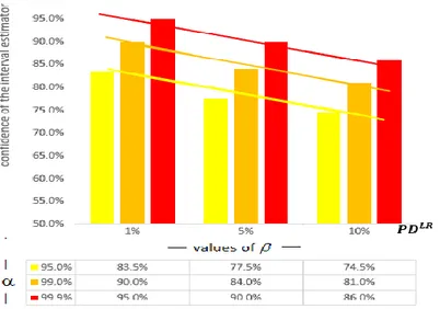
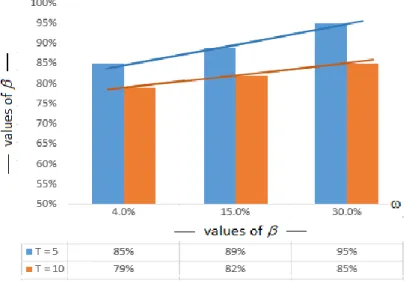
We derived the value of 𝛽 through Monte Carlo simulations for different combinations of the parameters 𝑃𝐷𝐿𝑅 and 𝜔 and for different numbers of default rates used to compute the estimator 𝐷𝑅̅̅̅̅. Figure 4 reports the value of 𝛽 obtained with 𝜔 = 0.3 and under the hypothesis that only 𝑇 = 5 observations of the default rates are used to estimate the 𝐷𝑅̅̅̅̅, which is the same setting involved in the stressed experiment of the previous section. Suppose we used 𝑇 = 5 observed default rates to estimate the 𝑃𝐷𝐿𝑅 for a given rating class and our estimate of
𝑃𝐷𝐿𝑅 were 5%, while 𝜔 = 30% was exogenously provided. If 5% were the true value of the probability of
default, then we could compute the 𝛼-quantile of the distribution of the default rates by means of (14) and we would be reasonably sure that the next year default rate will exceed this quantity with probability 1 − 𝛼. But we know that 5% is only an estimate and that there is uncertainty around this estimate. We can then exploit the expression (18) that contains a correction for the estimation variability. Figure 4 shows that the value of 𝛽 needed to obtain an adjusted-𝐷𝑅 value that will be exceed by the default rate with probability 0.1% (i.e. 𝛼 = 99.9%) is 90%. If instead the confidence level 𝛼 were 99% then the value of 𝛽 would be 84%; if 𝛼 = 95% then 𝛽 = 77%. Figure 4 .: Values of 𝛽 that ensure ℙ(𝐷𝑅𝑡> 𝑞̂ (𝐷𝑅𝛼,𝛽 𝑡)) = 1 − 𝛼: 𝛼 ∈ {95% . 99% . 99.9%}, 𝜔 = 0.3 and 𝑇 =
5
Figure 4 provides some interesting results. For a given values of 𝜔 and 𝑇, and with a given value of the confidence level 𝛼, the value of 𝛽 decreases as the probability of default increases. This implies that the level of conservativism required to account for the estimation error decreases with the value of the probability of default.
The second result is that the value of 𝛽 increases with the value of the confidence level 𝛼. For example, with 𝑃𝐷𝐿𝑅= 1%, 𝜔 = 30% and 𝑇 = 5, the value of 𝛽 needed to offset the estimation error is 𝛽 = 90% if 𝛼 = 99%
and 𝛽 = 97% if 𝛼 = 99.9%.
Furthermore in Figure 5 we study how the value of 𝛽 changes when the asset correlation 𝜔 changes. The figure shows that the value of 𝛽 required to ensure that ℙ(𝐷𝑅𝑡> 𝑞̂ ({𝐷𝑅𝛼,𝛽 𝑡})) = 1 − 𝛼 decreases when the number
𝑇 of annual default rates, used to compute 𝐷𝑅̅̅̅̅, increases. This result is not surprising since the variance of 𝐷𝑅̅̅̅̅ decreases with 𝑇. The value of 𝛽 increases with the asset correlation because the variance of 𝐷𝑅̅̅̅̅ is positively related with the asset correlation.
Figure 5.: Values of 𝛽 that ensure ℙ(𝐷𝑅𝑡> 𝑞̂ (𝐷𝑅𝛼,𝛽 𝑡)) = 1 − 𝛼: 𝛼 = 99.9% and 𝑃𝐷𝐿𝑅= 1%
Figure 4 and Figure 5 show the values of 𝛽 that satisfy the condition (19) under different values of the parameters. We obtained these values through Monte Carlo simulations: with the same approach, it would be possible to find the value of 𝛽 in any practical situation.
7. Empirical application
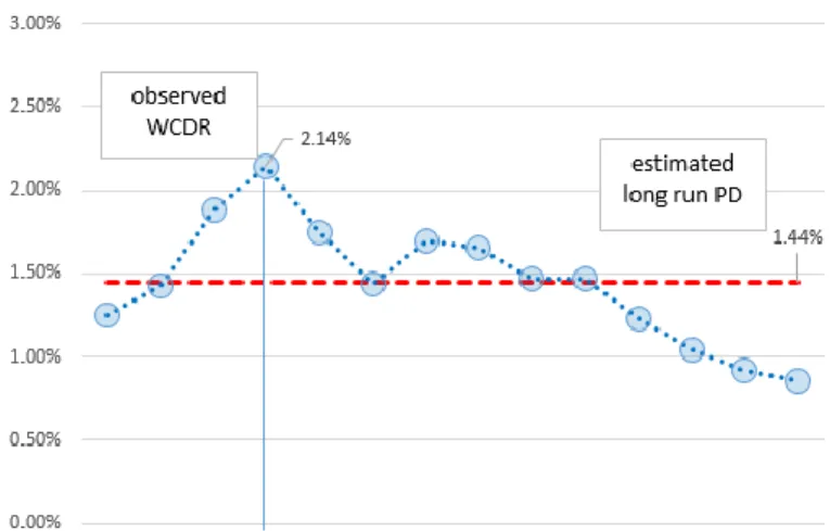
In this section we explore the relevance of the results with an empirical example based on real data. Figure 6 shows the annual default rates observed for the households sector in Italy. The time series spans a period of 𝑇 = 13 years. The average of the 13 observed default rates is equal to 𝐷𝑅̅̅̅̅ = 1.44%. This is the estimate of the long run probability of default 𝑃𝐷𝐿𝑅. In the figure it can be noticed that the observed worst default rate is equal to
2.14%.
Assume that the asset correlation is 𝜔 = 15%, which is the value attributed by the Regulators to mortgage portfolios. The observed default rates are referred to the households sector, which also includes other types of loans, like consumer loans and credit cards, but there is no doubt that residential mortgages represent a substantial component of the loans toward this sector. Table 2 shows that if we exploit the (14) with a confidence level 𝛼 = 99%, then the estimated worst-case default rate is equal to 8.19%. It is worth noticing that the estimated WCDR is about 4 times higher than the maximum default rate observed. By setting 𝛼 = 99.9% the estimated quantile is 14.19% (about 7 times the observed maximum default rate).
Table 2.: Estimated WCDR
𝑞𝛼=95%̂ ({𝐷𝑅𝑡}) 4.66%
𝑞𝛼=99%̂ ({𝐷𝑅𝑡}) 8.19%
𝑞𝛼=99.9%̂ ({𝐷𝑅𝑡}) 14.19%
We know that 𝐷𝑅̅̅̅̅ = 1.44% is only an estimate of the long run 𝑃𝐷 and we have seen that the variability of the estimator introduces an underestimation of the quantiles of the distribution of the default rates. So, for example, we may think that 𝑞̂ ({𝐷𝑅99.9% 𝑡}) = 14.2% is not enough to ensure that the default rates will exceed this quantity
with probability of 0.1%.
By means of (10) we can estimate that the variance of the default rates is 𝜎𝐷𝑅2 = 0.0257% and (13) shows that
the variance of the estimator 𝐷𝑅̅̅̅̅ is 𝜎𝐷𝑅2 /𝑇 = 0.00218%. Therefore, it is possible to define the upper bound of a
confidence interval estimator of the long run 𝑃𝐷 to endow the risk measure with an MoC to adjust for the estimation error. For example, with 𝛽 = 95% (16) provides the upper bounds of the interval estimator 𝑞𝛽=95%({𝐷𝑅̅̅̅̅}) = 1.44% + Φ−1(95%) ⋅ √0.00218% = 2.21%. In other words, we expect that the true value of
the 𝑃𝐷 is not higher than 2.21% with 95% of probability. We can use (18) to exploit the upper bound of the confidence interval, i.e. 2.21% instead of 1.44% in the Supervisory Formula. The result obtained is 𝑞𝛼=99.9%,𝛽=95%̂ ({𝐷𝑅𝑡}) = 18.8%. But we have seen that the value of 𝛽, that guarantees that the DR would not
exceed the stressed DR with a probability 99.9%, needs to be calibrated and it can be very different from 95%. Indeed, what emerged from the last section is that the correction needed to offset the estimation error must be calibrated on case by case basis as it is dependent on the level of the 𝑃𝐷 and asset correlation and also on the number of observations available for the computation of the average default rate.
We can then employ the Monte Carlo simulations to derive the level of 𝛽 needed to ensure that the probability of observing an exception (a default rate higher than the estimated quantile) is exactly equal to the desired level i.e. 1 − 𝛼. With an estimated 𝑃𝐷 equal to 1.44%, asset correlation of 15% and 𝑇 (the number of observed default rates) equal to 14, in Table 3 we obtain that the level of confidence for the interval estimator of the 𝑃𝐷 is 66% at the confidence level 95%; if 𝛼 is set to 99% then it is necessary to set 𝛽 = 70% and when 𝛼 = 99.9% then 𝛽 = 75%
Table 3.: estimated WCDR corrected for the estimation risk
𝑞𝛽=68%({𝐷𝑅̅̅̅̅}) 1.63% 𝑞𝛼=95%,𝛽=68%̂ ({𝐷𝑅𝑡}) 5.18%
𝑞𝛽=72%({𝐷𝑅̅̅̅̅}) 1.68% 𝑞𝛼=99%,𝛽=72%̂ ({𝐷𝑅𝑡}) 9.20%
𝑞𝛽=77%({𝐷𝑅̅̅̅̅}) 1.74% 𝑞𝛼=99.9%,𝛽=77%̂ ({𝐷𝑅𝑡}) 16.10%
In summary, according to (14) the estimate of the 99.9-quantile of the distribution of the default rates is 14.2% while according to (18) and setting 𝛽 = 75% it is 16.1%. The value of 𝛽 has been set to ensure that the probability of exceeding the identified threshold is 0.1%.
8. Conclusions
To quantify standard risk measures, such as Value-at-Risk (VaR), or Expected Shortfall, it is usually needed to substitute the theoretical models’ parameters with their estimated counterparts. Replacing, in the theoretical formulas, the true parameter value by an estimator induces estimation uncertainty and this can imply a significant underestimation of the required capital. The Prudential Regulators have raised the issue of errors stemming from the internal model estimation process in the context of credit risk, calling for margins of conservatism to cover possible underestimation in capital. In particular, a specific requirement can be found in Article 179 of EU Regulation 575/2013. Moreover, in the context of the ECB TRIM project, the banks’ approaches to quantify the MoC has been one of the items analysed and identified as a source of variability.
Estimation uncertainty in risk measures has been considered by several authors but few of them specifically dealt with the Asymptotic Single Risk Factor (ASRF) model that represents the baseline for the derivation of the credit risk measures under the Basel 2 IRB approach. In this paper, we study the effect of the estimation error in the ASRF framework and we show how to introduce a correction to control for the estimation error of the long run average probability of default. This simple and practical correction ensures that the probability of observing an exception (i.e. a default rate higher than the estimated quantile of the default rate distribution) is equal to the desired confidence level. The correction is obtained by substituting the value of the average default rate with the upper bound of an interval estimator. Our results point out that the confidence level of the interval estimator is not constant but varies with the number of default rates observed, the level of the asset correlation and the level of the probability of default. A feature of our approach is that we develop our reasoning remaining coherent with the ASRF framework without the need to introduce further hypotheses or other elements such as the prior distributions or other parameters which, having to be estimated, would introduce another source of estimation error.
We deem that the proposed correction is compliant with the general requirements required by the Regulation (Article 179 CRR) and the more specific requirements listed in the ECB guide to internal models. Indeed, the proposed correction depends on the distribution of the PD estimator, that we derived from the ASRF model’s underlying hypothesis, and the length of the time series. Furthermore, the simulation approach adopted to calibrate the correction also enables us to take into consideration the statistical uncertainty of each one-year default rate. We presented a practical application of our approach relying on real data. The results demonstrated that the impact of the correction can be material.
9.
Annex
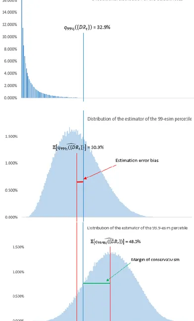
Figure 7 puts together the distribution of the annual default rates (first panel) and the distribution of the estimators 𝑞̂({𝐷𝑅99% 𝑡}) and 𝑞̂ ({𝐷𝑅99.9% 𝑡}) (second and third panel respectively). The first panel represents the distribution of the default rates given the parameters 𝜔 = 30%, 𝑇 = 5 and 𝑃𝐷 = 5%. It can be seen that the 99%-quantile of this distribution is equal to 32.9%. This value represents the WCDR, that is, the maximum default rate that is expected to be observed with a probability of 99%. The second panel shows the distribution of the random variable (14), that is an estimator of the 99%-quantile shown in the first panel. It can be seen that the expected value of this estimator is lower than the quantile, i.e. the estimator is downward biased. The last panel shows the distribution of the (14) with the confidence level 𝛽 set to 99.9%.
Figure 7.: Distribution of 𝐷𝑅𝑡. 𝑞̂({𝐷𝑅99% 𝑡})and 𝑞̂ ({𝐷𝑅99.9% 𝑡}) with 𝑃𝐷𝐿𝑅= 5%, 𝜔 = 0.3 , 𝑇 = 5 and 𝑁 =
Bibliography (References)
AIFIRM, (2019), The margin of conservativism (MOC) in the IRB approach, Position Paper 13. BCBS, (2006), International Convergence of Capital Measurement and Capital Standards. BCBS, (2005), An Explanatory Note on the Basel II IRB Risk Weight Functions.
Bluhm, C., Overbeck, L. and Wagner, C., (2010), Introduction to Credit Risk Modeling. (Second Edition). Chapman & Hall/CRC. London.
Christoffersen, P. and Gonçalves, S., (2005), Estimation Risk in Financial Risk Management. Journal of Risk, 7, 1-28.
EBA, (2017), Guidelines on PD estimation, LGD estimation and the treatment of defaulted exposures ECB (2018), ECB guide to internal models: Risk type specific chapters.
Escanciano, J. Carlos & Olmo, Jose, 2010. Backtesting Parametric Value-at-Risk With Estimation Risk, Journal of Business & Economic Statistics, American Statistical Association, vol. 28(1), pages 36-51
EU (2013), European Parliament and Council, Regulation (EU) No 575/2013, Official Journal of the European Union
Figlewski, S., (2004), Estimation Error in the Assessment of Financial Risk Exposure. Working paper, New-York University.
Gouriéroux, C., and Zakoïan, J., (2012), Estimation Adjusted VaR. Annales d’Economie et de Statistique, 78, 1–33. Jorion, P., (2007), Value at Risk. The New Benchmark for Managing Financial Risk. (Third Edition). MacGraw-Hill, New York.
Landini, S., Gallegati M., and Rosser, J.B. Jr., (2020), Consistency and Incompleteness in General Equilibrium Theory. Journal of Evolutionary Economics. Vol. 30: 205-230.
Tarashev, N., (2009), Measuring portfolio credit risk correctly: why parameter uncertainty matters, BIS Working Papers, vol. 280.
ACKNOWLEDGEMENTS
We are grateful to M. Mancini and G. Rinna for useful comments and suggestions on a preliminary draft of the paper.
The opinions expressed are those of the authors and not involve responsibility of the institutions.
Simone Casellina:
Bank sector analyst, European Banking Authority
Simone Landini:
Senior researcher, Quantitative methods for economics and finance; IRES Piemonte
Mariacristina Uberti:
Full professor of Mathematical Finance; Department of Management, University of Turin
EUROPEAN BANKING AUTHORITY
20 avenue André Prothin CS 30154 92927 Paris La Défense CEDEX, France Tel. +33 1 86 52 70 00 E-mail: [email protected] https://eba.europa.eu/ ISBN 978-92-9245-728-0 ISSN 2599-7831 10.2853/032235 DZ-AH-21-001-EN-N © European Banking Authority, 2021.
Any reproduction, publication and reprint in the form of a different publication, whether printed or produced electronically, in whole or in part, is permitted, provided the source is acknowledged. Where copyright vests in a third party, permission for reproduction must be sought directly from the copyright holder.
This paper exists in English only and it can be downloaded without charge from
https://www.eba.europa.eu/about-us/staff-papers, where information on the EBA Staff Paper Series can also be found.