How to catch scaling in geophysics : some problems in stochastic modelling and inference from time series

SCIENZE DELL’INGEGNERIA CIVILE

SCUOLA DOTTORALE

XXV

CICLO DEL CORSO DI DOTTORATO

How to catch scaling in geophysics: some problems in

stochastic modelling and inference from time series

Titolo della tesi

Federico Lombardo

__________________

Nome e Cognome del dottorando

Elena Volpi

__________________

Docente Guida/Tutor: Prof.

Aldo Fiori

__________________

ii

Collana delle tesi di Dottorato di Ricerca In Scienze dell’Ingegneria Civile

Università degli Studi Roma Tre Tesi n° 46

iii

L'arte e la scienza sono libere e libero ne è l'insegnamento.

Sommario

Nel corso degli ultimi decenni lo studio dei cambiamenti nei processi geofisici ha riscosso un crescente interesse soprattutto in riferimento alle potenziali ripercussioni sulla nostra società. Lo scopo primario è di migliorare il processo di previsione di tali cambiamenti per consentire uno sviluppo sostenibile delle attività umane in un ambiente mutevole. Le variazioni dei processi geofisici sono presenti a tutte le scale temporali e sono irregolari a tal punto che la loro descrizione può certamente essere migliore in termini stocastici (casuali) che deterministici. Nella statistica classica, la casualità viene solitamente rappresentata da processi stocastici le cui variabili casuali sono indipendenti ed identicamente distribuite. Tuttavia, esiste un’ampia evidenza empirica che spesso confuta tale assunzione. Infatti, è stato osservato in più occasioni che la correlazione tra campioni sempre più distanti tra loro nel tempo decresce più lentamente non solo di quanto ovviamente ci si aspetta per campioni indipendenti ma anche rispetto al caso di dipendenza markoviana o dei modelli di tipo ARMA. Tutto ciò è coerente con il fenomeno di Hurst, che è stato infatti osservato in molte lunghe serie temporali idroclimatiche. Esso è stocasticamente equivalente ad un comportamento auto-simile della variabilità del processo alle differenti scale temporali. Di conseguenza, i cambiamenti persistenti a lungo termine sono molto più frequenti ed intensi nei processi geofisici di quanto comunemente percepito e, inoltre, gli stati futuri sono molto più incerti ed imprevedibili su lunghi orizzonti temporali rispetto alle previsioni ottenute mediante i modelli tipicamente utilizzati nella pratica. L’obiettivo della presente tesi è la descrizione dell’inferenza e della modellazione delle proprietà statistiche relative ai processi naturali che presentano un comportamento del tipo scala invariante. Dapprima si indagano le ripercussioni che tale comportamento implica in riferimento all’ingente incremento di incertezza di stima dei parametri di interesse dalle serie temporali di dati. In seguito viene proposto un modello stazionario di disaggregazione temporale della precipitazione che rispetta il fenomeno di Hurst. Tale modello è caratterizzato da una semplice struttura a cascata simile a quella dei più famosi modelli a cascata moltiplicativa di tipo discreto. Inoltre mostriamo il grande limite di questi ultimi modelli che simulano un processo intrinsecamente non stazionario a causa della loro struttura.

v

Abstract

During recent decades, there has been a growing interest in research activities on change in geophysics and its interaction with human society. The practical aim is to improve our capability to make predictions of geophysical processes to support sustainable societal development in a changing environment. Geophysical processes change irregularly on all time scales, and then this change is hardly predictable in deterministic terms and demands stochastic descriptions, or random. The term randomness is usually associated to stochastic processes whose samples are regarded as a sequence of independent and identically distributed random variables. This is a basic assumption of classical statistics, but there is ample practical evidence that this wish does not always become a reality. It has been observed empirically that correlations between distant samples decay to zero at a slower rate than one would expect from not only independent data but also data following classical ARMA- or Markov-type models. Indeed, many geophysical changes are closely related to the Hurst phenomenon, which has been detected in many long hydroclimatic time series and is stochastically equivalent to a simple scaling behaviour of process variability over time scale. As a result, long-term changes are much more frequent and intense than commonly perceived and, simultaneously, the future states are much more uncertain and unpredictable on long time horizons than implied by typical modelling practices. The purpose of this thesis is to describe how to infer and model statistical properties of natural processes exhibiting scaling behaviours. We explore their statistical consequences with respect to the implied dramatic increase of uncertainty, and propose a simple and parsimonious model that respects the Hurst phenomenon. In particular, we first we highlight the problems in inference from time series of geophysical processes, where scaling behaviours in state (sub-exponential distribution tails) and in time (strong time dependence) are involved. Then, we focus on rainfall downscaling in time, and propose a stationary model that respects the Hurst phenomenon. It is characterized by a simple cascade structure similar to that of the most popular multiplicative random cascade models, but we show that the latter simulate an unrealistic non-stationary process simply inherent to the model structure.

vi

Table of contents

LIST OF FIGURES ... VII LIST OF SYMBOLS ... XI

1. INTRODUCTION ... 1

1.1 JOSEPH EFFECT AND HURST EFFECT ... 5

1.2 STOCHASTIC MODELLING OF CHANGE ... 7

1.3 HURST-KOLMOGOROV PROCESS ... 9

1.4 CLIMACOGRAM... 13

1.5 OUTLINE OF THE THESIS ... 15

2. GEOPHYSICAL INFERENCE ... 16

2.1 MULTIFRACTAL ANALYSIS... 18

2.1.1 ESTIMATION OF THE MEAN ... 20

2.1.2 ESTIMATION OF HIGHER MOMENTS ... 21

2.1.3 MONTE CARLO SIMULATION ... 23

2.1.4 EMPIRICAL MOMENT SCALING FUNCTION ... 29

2.1.5 OVERVIEW OF KEY IDEAS ... 33

2.2 SAMPLING PROPERTIES OF CLIMACOGRAM AND POWER SPECTRUM ... 35

2.2.1 SOME THEORETICAL CONSIDERATIONS ... 36

2.2.2 ASYMPTOTIC PROPERTIES OF THE POWER SPECTRUM ... 38

2.2.3 POWER SPECTRUM ESTIMATION ... 41

2.2.4 CLIMACOGRAM ESTIMATION ... 44

2.2.5 OVERVIEW OF KEY IDEAS ... 47

3. RAINFALL DOWNSCALING ... 49

3.1 MULTIPLICATIVE RANDOM CASCADE MODELS ... 51

3.1.1 DOWNSCALING MODEL (CANONICAL CASCADE) ... 53

3.1.2 EXAMPLE: NUMERICAL SIMULATION ... 56

3.1.3 DISAGGREGATION MODEL (MICRO-CANONICAL CASCADE) ... 59

3.1.4 BOUNDED RANDOM CASCADES ... 59

3.2 HURST-KOLMOGOROV DOWNSCALING MODEL ... 60

3.2.1 EXAMPLE: NUMERICAL SIMULATION ... 65

3.2.2 APPLICATION TO AN HISTORICAL OBSERVED EVENT ... 67

3.3 HK DISAGGREGATION MODEL ... 71

3.4 OVERVIEW OF KEY IDEAS ... 75

4. CONCLUSIONS AND DISCUSSION ... 77

ACKNOWLEDGEMENTS ... 82

vii

List of figures

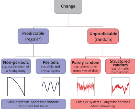
1.1 Hierarchical chart describing the predictability of change

(Koutsoyiannis, 2013a). 2

1.2 Plot of standardized tree rings at Mammoth Creek, Utah (upper panel); white noise with same statistics (lower panel) (Koutsoyiannis, 2002). 4

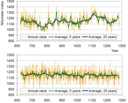
1.3 Plot of annual minimum water level of the Nile river (upper panel); white noise with same statistics (lower panel)

(Koutsoyiannis, 2002). 4

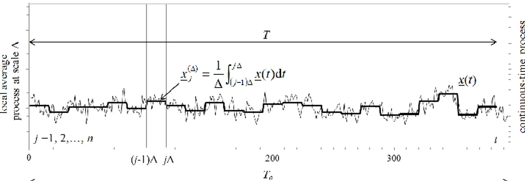
1.4 Sketch of the local average process xj(Δ) obtained by

averaging the continuous-time process x(t) locally over

intervals of size Δ. 10

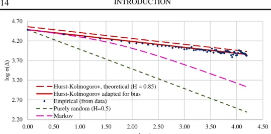
1.5 Climacogram of Nilometer data and fitted theoretical ones of white noise (H=0.5), Markov and HK process (adapted

from Koutsoyiannis, 2013a). 14

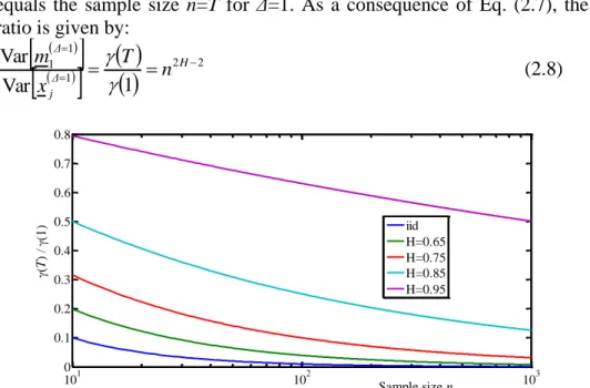
2.1 Estimator variance of the mean of the local average process xj(Δ=1) standardized by the process variance, i.e.

Var[m1(Δ=1)]/Var[xj(Δ=1)]=γ(T)/γ(1), plotted against the

sample size n=T for Δ=1. 21

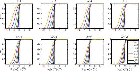
2.2 Empirical cumulative distribution function (ecdf) of the natural logarithm of the ratio of q-th moment estimates to their expected values E[(xj(Δ))q]=μq(Δ) when varying Δ. 24

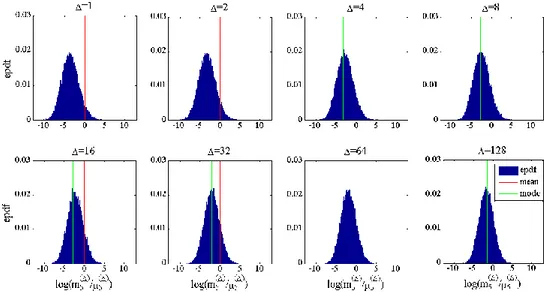
2.3 Empirical probability density function (epdf) of the sample 5-th moment estimated from lognormal time series averaged locally over different timescales Δ. 25

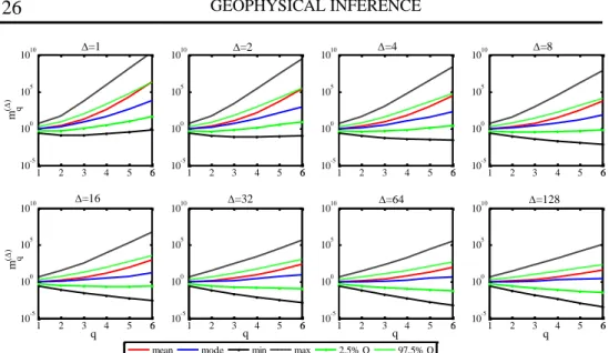
2.4 Semi-logarithmic plots of the prediction intervals of the sample moments versus the order q for various timescales

viii

2.5 Log-log plots of the prediction intervals of the sample moments versus the scale Δ for various orders q. 26

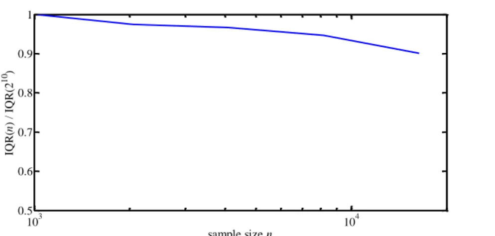
2.6 Semi-logarithmic plot of the interquartile range (IQR) (standardized with respect to the IQR for n=210_{) of the}

prediction intervals for the third moment versus the sample size n for the lognormal series generated by our downscaling model (see Sect. 3.2). 27

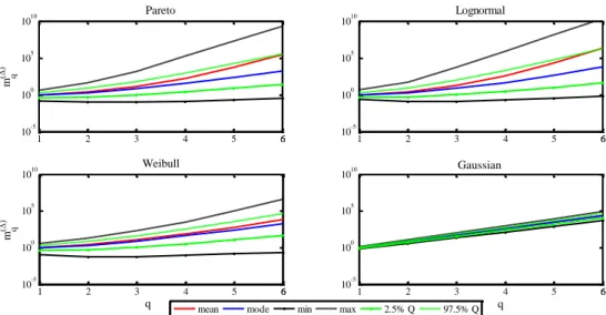
2.7 Semi-logarithmic plots of the prediction intervals of the sample moments versus the order q for various marginal probability distributions, assuming Δ=1. 28

2.8 Prediction intervals of the moment scaling function K(q) versus the order q for lognormal series generated by our downscaling model (Sect. 3.2). 30

2.9 Comparison between theoretical (true) and empirical (estimated) power spectra of a time series of 1024 values generated from the Cauchy-type process defined by Eq.

(2.60). 43

2.10 Comparison between theoretical (true) and empirical (estimated) climacograms of a time series of 1024 values generated from the Cauchy-type process defined by Eq.

(2.60). 46

2.11 Comparison between empirical and theoretical spectra and pseudospectra for the Cauchy-type process defined by Eq.

(2.60). 47

3.1 Sketch of a dyadic (b = 2) multiplicative random cascade. 53

3.2 Example of computation of the exponent hj,k(z) for a

canonical MRC. In the computation we use Eq. (3.14) and the arrows indicate the links to those variables considered. 55

3.3 Ensemble mean of the example MRC process as a function of the position j along the cascade level k = 7. 57

ix 3.4 Ensemble standard deviation of the example MRC process

as a function of the position j along the cascade level k = 7. 57

3.5 Ensemble autocorrelation function of the example MRC process at the cascade level k = 7 with starting point j (for j=1, n/4 and n/2, respectively, from left to right) in the considered cascade level with n = 27 _{= 128 elements. 58}

3.6 ACF of the example MRC process at the cascade level k = 7 with starting point j = n/2 (left) and j = n/2+2 (right) zoomed in the lag range [–5, 5]. 58

3.7 Example of the dyadic additive cascade for four disaggregation levels (k = 0, 1, 2, 3), where arrows indicate the links to those variables considered in the current generation step (adapted from Koutsoyiannis, 2002). 61

3.8 Ensemble mean of the example HK process as a function of the position j along the cascade level k = 7. 66

3.9 Ensemble standard deviation of the example HK process as a function of the position j along the cascade level k = 7. 66

3.10 Ensemble autocorrelation function of the example HK process at the cascade level k = 7 with starting point j (for j=1, n/4 and n/2, respectively, from left to right) in the considered cascade level with n = 27 _{= 128 elements. 67}

3.11 Hyetograph of the historical rainfall event (no. 3) measured in Iowa on 30 November 1990 (upper panel; Georgakakos et al., 1994) along with two synthetic time series of equal length generated by the MRC and HK models (middle and lower panels, respectively). 68

3.12 Double logarithmic plot of the standard deviation σ(Δ) of the aggregated process Xj(Δ) vs. scale Δ (climacogram) for

both the real and the log-transformed data of the Iowa rainfall event (upper panel); climacograms of the 1st and the 99th percentiles for the HK downscaling model (10000 69

x

Monte Carlo experiments) and for the observed rainfall event (lower panel).

3.13 Empirical autocorrelation function (ACF) of the Iowa rainfall event examined and 1st and 99th percentiles of ACF for the HK downscaling model. 70

3.14 Ensemble mean of the example HK disaggregation process as a function of the position j along the cascade level k = 7. 73

3.15 Standard deviation of the example HK disaggregation

process. 73

3.16 Ensemble autocorrelation function of the example HK process at the cascade level k = 7 with starting point j (for j=1, n/4 and n/2, respectively, from left to right) in the considered cascade level with n = 27 _{= 128 elements. 74}

3.17 Scatter plot of the calculated sum of the lower-level variables (before, blue, and after, green, applying the adjusting procedure) vs. the given values of the higher-level variables X1,0 for all Monte Carlo experiments. 74

xi

List of symbols

Δ Time scale j Discrete time step RΔ Adjusted range H Hurst coefficient t Continuous time

BH Fractional Brownian motion x(t) Instantaneous process

xj(Δ) Local average process over the time window Δ at discrete time steps j

X(t) Cumulative process in continuous time Xj(Δ) Aggregated process on a time scale Δ n Sample size

To Observation period (in continuous time) T Observation period (in discrete time) μ Mean of a stochastic process

mq(Δ) Estimator of the q-th raw moment of the local average process xj(Δ) μq(Δ)

Theoretical raw moment of order q of the local average process xj(Δ) γ(Δ) Variance of the time-averaged process xj(Δ) as a function of the time

scale of averaging Δ

σ(Δ) Standard deviation of the time-averaged process xj(Δ) as a function of the time scale of averaging Δ

xii

g(Δ) Sample variance

λ Scale ratio λ so that λ=1 for the largest scale of interest Δmax, i.e. λ=Δmax/Δ.

ε(λ) Non-dimensional process obtained dividing the process xj(Δ) by its mean at the largest scale Δmax (or equivalently λ=1)

s(w) Power spectrum of the continuous-time (instantaneous) process, where w is the frequency

sd(Δ)(ω) Power spectrum of the discrete-time process, where ω = wΔ is nondimensionalized frequency

s#(w) The asymptotic slopes of the power spectrum s(w)

c(τ) Autocovariance function for the continuous-time process Cov[x(t), x(t+τ)], where τ is the continuous time lag

ρ(τ) Autocorrelation function for the instantaneous process

cz(Δ) Autocovariance function for the averaged process Cov[xj(Δ), xj+z(Δ)] (with c0(Δ)=γ(Δ)), where z is the discrete time lag

ρ(Δ)_{(z) Autocorrelation function for the averaged process, where z is the} discrete time lag

ψ(w) The climacogram-based pseudospectrum (CBPS) ψ#

(w) The asymptotic logarithmic slope of CBPS

x1,0 Average rainfall intensity over time scale fΔ at the time origin (j=1),

i.e. x1(fΔ) (start vertex of the random cascade) μ0, γ0 Mean and variance of x1,0

b Branching number of the random cascade k Level of the cascade

wj,k Random weight in the position j at the level k of the multiplicative cascade

xiii μw, γw Common mean and variance of the cascade weights wj,k

xj,k Generic vertex of the cascade μj,k, γj,k Mean and variance of xj,k

ρj,k(z) The autocorrelation function for discrete-time lag z between two vertices of the cascade

hj,k(z) Exponent of formula of ρj,k(z), which determines its dependence on the position j in the cascade

X1(f) Cumulative rainfall depth at the time origin (j=1) aggregated on the largest time scale f (i.e., fΔ but Δ is omitted for convenience); it assumed log-normally distributed

0 , 1

~

X _{Auxiliary Gaussian random variable}  f  f X

X~₁ ln ₁ of the aggregated HK process on the time scale f (start vertex of the random additive cascade)

θ Vector of parameters of the HK downscaling model

α(k), β(k) Scale-dependent functions derived to preserve the scaling properties of the actual (exponentiated) process

INTRODUCTION 1

1. Introduction

Discipulus est prioris posterior dies.

Publilius Syrus

Change in geophysics has been studied since the birth of science and philosophy, but in modern times change has been particularly accelerated due to radical developments in demography, technology and life conditions. Therefore, during recent decades, there has been a growing interest in research activities on change in geophysics and its interaction with human society. A major example in this respect is given by the Intergovernmental Panel on Climate Change (IPCC), which was set up in 1988 by the World Meteorological Organization (WMO) and United Nations Environment Programme (UNEP) to provide policymakers with regular assessments of the scientific basis of climate change, its impacts and future risks, and options for adaptation and mitigation. Furthermore, the new scientific initiative of the International Association of Hydrological Sciences (IAHS) for the decade 2013–2022, entitled “Panta Rhei – Everything Flows” (Montanari et al., 2013), is dedicated to research activities on change in hydrology and society.

The practical purpose of all these activities is to improve our capability to make predictions of geophysical processes to support sustainable societal development in a changing environment. In order to describe the predictability of change, we adopt herein an interesting hierarchical chart by Koutsoyiannis (2013a) reported in Fig. 1.1. Change is regular in simple systems (left part of the graph), and therefore it is predictable using equations of dynamical systems (periodic or aperiodic). Nonetheless, in geophysics we are commonly interested in more complex systems with long time horizons (right part of the graph), where change is unpredictable in deterministic terms, or random. The term randomness is usually associated to stochastic processes whose samples are regarded as a sequence of independent and identically distributed random variables (pure randomness). This is a basic assumption of classical statistics, but there is ample practical evidence that this wish does not always become a reality (Beran, 1994). By the way, it has been observed empirically that correlations between distant samples decay to zero at a slower rate than one would expect from independent data or even data following classical

INTRODUCTION

2

ARMA- or Markov-type models (Box et al., 1994). In these cases, we should assume a structured randomness. As will be seen next, the structured randomness is enhanced randomness, expressing enhanced unpredictability of enhanced multi-scale change.

Figure 1.1 – Hierarchical chart describing the predictability of change (Koutsoyiannis, 2013a).

According to the common view, natural processes are composed of two different, usually additive, parts or components: deterministic (signal) and random (noise). This distinction implies that there is some signal that contains information, which is contaminated by a (random) noise. In this view, randomness is cancelled out at large time scales and cannot produce long-term change. In other words, we usually assume that natural changes are just a short-term “noise” superimposed on the daily and annual cycles in a scene that is static and invariant in the long run, except when an extraordinary forcing produces a long-term change. However, this view may not have a meaning in geophysics, as Nature’s signs are “signals” in their entirety even though they may look like “noise”. Moreover, change occurs on all time scales, from minute to geological, but our limited

INTRODUCTION 3 senses and life span, as well as the short time window of instrumental observations, restrict our perception to the most apparent daily to yearly variations. As a result, long-term changes are much more frequent and intense than commonly perceived and, simultaneously, the future states are much more uncertain and unpredictable on long time horizons than implied by standard approaches (Markonis and Koutsoyiannis, 2013). We endorse herein a different perspective (see also Koutsoyiannis, 2010). Randomness is simply viewed as unpredictability and coexists with determinism (which, in turn, could be identified with predictability) in the same natural process: the two do not imply different types of mechanisms or different parts or components in the time evolution, they are not separable or additive components. It is a matter of specifying the time horizon and scale of prediction to decide which of the two dominates. For long time horizons (where the specific length depends on the system), all is random – and not static.

Empirical evidence suggests that long historical hydroclimatic series may exhibit a behaviour very different from that implied by pure random models. To demonstrate this, two real-world examples are used (Koutsoyiannis, 2002). The first is a very long record: the series of standardised tree-ring widths from a palaeoclimatology study at Mammoth Creek, Utah, for the years 0–1989 (1990 values) (Graybill, 1990). The second example is the most intensively studied series, which also led to the discovery of the Hurst phenomenon (Hurst, 1951): the series of the annual minimum water level of the Nile River for the years 622–1284 A.D. (663 observations), measured at the Roda Nilometer near Cairo (Toussoun, 1925; Beran, 1994). The data values are plotted vs time for both example data sets in Figs. 1.2 and 1.3, respectively. In addition, the 5-year and 25-year averages are shown, which represent the mean aggregated processes at time scales Δ = 5 and 25, respectively. For comparison, series of white noise with mean and standard deviation identical to those of standardized tree rings and annual minimum water levels are also shown. It is observed that fluctuations of the aggregated processes, especially for Δ = 25, are much greater in the real-world time series than in the white noise series. Thus, the existence of fluctuations in a time series at large scales distinguishes it from random noise. When one looks only at short time periods, then there seem to be cycles or local trends. However, looking at the whole series, there is no apparent persisting trend or cycle. It rather seems that cycles of (almost) all frequencies occur, superimposed and in random sequence.

INTRODUCTION

4

Figure 1.2 – Plot of standardized tree rings at Mammoth Creek, Utah (upper panel); white noise with same statistics (lower panel) (Koutsoyiannis, 2002).

Figure 1.3 – Plot of annual minimum water level of the Nile river (upper panel); white noise with same statistics (lower panel) (Koutsoyiannis, 2002).

INTRODUCTION 5 From the figures above, it can be noticed that in pure randomness (white noise) there are no long-term patterns; rather, the time series appear static in the long run. In real-world data, change is evident also at these scales. This change is unpredictable in deterministic terms and thus random and, more specifically, structured (or enhanced) random rather than purely random (Koutsoyiannis, 2013a).

1.1 Joseph effect and Hurst effect

The data sets in the previous section illustrated that correlations not only occur, but they also may persist for a long time. Many prominent applied statisticians and scientists recognized this many decades ago. In this section, we give a short overview on some of the important early references. This will also give rise to some principal considerations on the topic of long-range dependence.

Since ancient times, the Nile River has been known for its characteristic long-term behaviour. Long periods of dryness were followed by long periods of yearly returning floods. Floods had the effect of fertilising the soil so that in flood years the yield of crop was particularly abundant. On a speculative basis, one may find an early quantitative account of this in the Bible (Genesis 41, 29-30): “Seven years of great abundance are coming throughout the land of Egypt, but seven years of famine will follow them”. We do not have any records of the water level of the Nile from those times. However, there are reasonably reliable historical records going as far back as 622 A.D. A data set for the years 622–1284 was discussed in the previous section (see Fig. 1.3, upper panel). It exhibits a long-term behavior that might give an “explanation” of the seven “good” years and seven “bad” years described in Genesis. There were long periods where the maximal level tended to stay high. On the other hand, there were long periods with low levels. Overall, the series seems to correspond to a stationary stochastic process, where there is no global trend. In reference to the biblical “seven years of great abundance” and “seven years of famine”, Mandelbrot called this behaviour the Joseph effect (Mandelbrot, 1982; Mandelbrot and Wallis 1968, 1969; Mandelbrot and van Ness, 1968).

The first person to notice this behavior empirically was the British hydrologist H. E. Hurst (1951), when he was investigating the question of how to regularize the flow of the Nile River. More specifically, his discovery can be described as follows. Suppose we want to calculate the

INTRODUCTION

6

capacity of a reservoir such that it is ideal for a given time span; assume that time is discrete and that there are no storage losses (caused evaporation, leakage, etc.). By ideal capacity, we mean that the outflow is uniform, that the water level in the reservoir is constant, and that the reservoir never overflows. Let xj denote the inflow at time j (notice that

we use the so-called Dutch convention according to which random variables are underlined; see Hemelrijk, 1966), and the partial sum yΔ=x1+x2+…+xΔ is the cumulative inflow up to time Δ, for any integer Δ.

Then the ideal capacity can be shown to equal the adjusted range (Yevjevich, 1972):       _        _     j Δ j Δ j Δ j Δ Δ y Δ j y y Δ j y R 1 1 min max : (1.1)

In order to study the properties that are independent of the scale Δ, RΔ is

standardised by the sample standard deviation SΔ of xj. This ratio is called

the rescaled adjusted range or R/S-statistic. Hurst plotted the logarithm of R/S against several values of Δ. He observed that, for large values of Δ, log R/S was scattered around a straight line with a slope greater than 0.5. This empirical finding was in contradiction to results for Markov processes, mixing processes, and other stochastic processes that were commonly used at that time. For any stationary process with short-range dependence, R/S should be asymptotically proportion al to Δ0.5 (Beran, 1994). Analogous considerations apply to many other geophysical records for which R/S is asymptotically proportional to ΔH _{for H > 0.5. This is}

known as Hurst effect. Strikingly, the preeminent Soviet mathematician and physicist A. N. Kolmogorov had proposed a mathematical process that has the properties discovered 10 years later by Hurst in natural processes (Kolmogorov, 1940). Although the original name given by Kolmogorov was “Wiener’s spiral”, it later became more widely known by “fractional Brownian motion” or “fractional Gaussian noise” for the stationary increment process (Mandelbrot and van Ness, 1968). The latter is what we call hereinafter the Hurst-Kolmogorov (HK) process. The Hurst effect can be modelled by HK process with self-similarity (see next section) parameter 0.5 < H < 1 (Hurst coefficient).

The reason why we prefer the term Hurst-Kolmogorov process is simple. We wish to associate the process on the one hand to Hurst, who was the first to observe and analyze the behaviour signified by this process in Nature, and on the other hand, to Kolmogorov, who was the first to point out the existence of this mathematical process. For a detailed review and

INTRODUCTION 7 discussion of the names given to the Hurst phenomenon and its mathematical modelling, the reader is referred to Koutsoyiannis (2006). This Hurst-Kolmogorov process is a model that simulates a stationary stochastic process.

A stochastic process x(t) is called stationary if its statistical properties are invariant to a shift of the time origin (Papoulis, 1991). This means that the processes x(t) and x(t+τ) have the same statistics for any τ. Conversely, a process is non-stationary if some of its statistics are changing through time and their change is described as a deterministic function of time. From a scientific point of view, it is not always satisfactory to model an observed phenomenon by a stationary process. For example, Klemeš (1974) showed that the Hurst phenomenon could be caused by non-stationarity in the mean and by random walks with one absorbing barrier. However, we would most likely want to use a stationary model as a null hypothesis unless physical considerations determined otherwise. Indeed, Koutsoyiannis (2002) offered a similar (from a practical point of view) explanation to that given by Klemeš (1974), but in a stationary setting. In essence, he assumed that the means are randomly varying on several timescales, thus regarding falling or rising trends, commonly traced in hydrological time series, as parts of large-scale random fluctuations rather than deterministic trends.

1.2 Stochastic modelling of change

In this section, we introduce stochastic processes that can be used to model data with the properties discussed in previous sections.

A simple way to understand the extreme variability of several geophysical processes over a practically important range of scales is offered by the idea that the same type of elementary process acts at each relevant scale. In a theoretical context, Kolmogorov (1940) introduced these types of processes that go under the name of “self-similar processes”, which are based on a form of invariance with respect to changes of time scale. According to this idea, the part resembles the whole as quantified by so-called “scaling laws”. Scaling behaviours are typically represented as power laws of some statistical properties, and they are applicable either on the entire domain of the variable of interest or asymptotically. If this random variable represents the state of a system, then we have the scaling in state, which refers to marginal distributional properties. This is to distinguish from another type of scaling, which deals with time-related

INTRODUCTION

8

random variables: the scaling in time, which refers to the dependence structure of a process. Likewise, scaling in space is derived by extending the scaling in time in higher dimensions and substituting space for time (e.g. Koutsoyiannis et al., 2011). The scaling behaviour widely observed in the natural world (e.g. Newman, 2005) has often been interpreted as a tendency, driven by the dynamics of a physical system, to increase the inherent order of the system (self-organized criticality): this is often triggered by random fluctuations that are amplified by positive feedback (Bak et al., 1987). In another view, the power laws are a necessity implied by the asymptotic behaviour of either the survival or autocovariance function, describing, respectively, the marginal and joint distributional properties of the stochastic process that models the physical system. The main question is whether the two functions decay following an exponential (fast decay) or a power-type law (slow decay). We assume the latter to hold in the form of scaling in state (heavy-tailed distributions) and in time (long-term persistence), which have also been verified in geophysical time series (e.g. Markonis and Koutsoyiannis, 2013; Papalexiou et al., 2013). According to this view, scaling behaviours are just manifestations of enhanced uncertainty and are consistent with the principle of maximum entropy (Koutsoyiannis, 2011). The connection of scaling with maximum entropy constitutes also a connection of stochastic representations of natural processes with statistical physics. The emergence of scaling from maximum entropy considerations may thus provide theoretical background in modelling complex natural processes by scaling laws.

Since Kolmogorov’s pioneering work, several researchers do not seem to have been aware of the existence or statistical relevance of such processes, until Mandelbrot and van Ness (1968) introduced them into statistics: “By ‘fractional Brownian motions’ (fBm’s), we propose to designate a family of Gaussian random functions defined as follows: B(t) being ordinary Brownian motion, and H a parameter satisfying 0<H<1, fBm of exponent H [denoted as BH(t)] is a moving average of dB(t), in

which past increments of B(t) are weighted by the kernel (t–s)H–1/2_{”. As}

usual, t designates time, –∞<t< ∞.

The increment process, x(t2–t1)=BH(t2)–BH(t1), is stationary and

self-similar with parameter H, it is known as fractional Gaussian noise (i.e. Hurst-Kolmogorov process), and it is given by (see Mandelbrot and van Ness, 1968, p. 424):

INTRODUCTION 9



_{ }

_





 





 





which is a fractional integral in the sense of Weyl. The gamma function Γ(·) as denominator insures that, when H – 0.5 is an integer, a fractional integral becomes an ordinary repeated integral.

The value of the Hurst coefficient H determines three very different families of HK processes, corresponding, respectively, to: 0<H<0.5, 0.5<H<1, and H=0.5. The value 0.5 corresponds to white noise. For geophysical processes, we restrict ourselves to a discussion of HK processes positively correlated, i.e. 0.5<H<1. Values H<0.5, characteristic of anti-persistence, are mathematically feasible (in discrete time) but physically unrealistic; specifically, for 0<H<0.5 the autocorrelation for any lag is negative, while for small lags a physical process should necessarily have positive autocorrelation. High values of H, particularly those approaching 1, indicate enhanced change at large scales or strong clustering (grouping) of similar values, otherwise known as long-term persistence. In other words, in a stochastic framework and in stationary terms, change can be characterized by the Hurst coefficient.

1.3 Hurst-Kolmogorov process

The original Hurst’s mathematical formulation, in terms of the so-called rescaled range, involves complexity and estimation problems as shown by Koutsoyiannis (2002). Actually, the mathematics to describe the HK process may be very simple. No more than the concept of standard deviation from probability theory is needed. Because a static system whose response is a flat line (no change in time) has zero standard deviation, we could recognize that the standard deviation is naturally related to change. To study change, however, we need to assess the standard deviation at several time scales, i.e. the relationship of the process standard deviation with the temporal scale of the process.

In order to improve understanding of Hurst-Kolmogorov process, we should describe the concept of “local average” of a stochastic process. Practical interest often revolves around local average or aggregates (temporal or spatial) of random variables, because it is seldom useful or necessary to describe in detail the local point-to-point variation occurring on a microscale in time or space. Even if such information were desired, it may be impossible to obtain: there is a basic trade-off between the

INTRODUCTION

10

accuracy of a measurement and the (time or distance) interval within which the measurement is made (Vanmarke, 1983). For example, rain gauges (owing to size, inertia, and so on) measure some kind of local average of rainfall depth over time. Moreover, through information processing, "raw data" are often transformed into average or aggregate quantities such as, e.g., sub-hourly averages or daily totals.

Mathematically, let x(t) be a stationary stochastic process in continuous time t with mean μ=E[x], and autocovariance c(τ)=Cov[x(t), x(t+τ)], where τ is the time lag. Consider now the random process xj(Δ) obtained by

local averaging x(t) over the window Δ at discrete time steps j (=1, 2, …), defined as:  

_{ }

_

where n=T/Δ is the number of the sample steps of xj(Δ) in the observation

period To, and T 





integer multiple of Δ. The relationship between the processes x(t) and xj(Δ)

is illustrated in Fig. 1.4.

Figure 1.4 – Sketch of the local average process xj(Δ) obtained by averaging the

continuous-time process x(t) locally over intervals of size Δ.

The mean of the process xj(Δ) is not affected by the averaging operation,

i.e.:  

 



 

 

Let us now investigate the climacogram of the process xj(Δ), which is

defined to be the variance (or the standard deviation) of the time-averaged process xj(Δ) as a function of the time scale of averaging Δ (Koutsoyiannis,

INTRODUCTION 11 function c(τ) of the continuous-time process as follows (see e.g. Vanmarke, 1983, p. 186; Papoulis, 1991, p. 299):  

 

 

_



  

_



  

which shows that the climacogram γ(Δ) generally decreases with Δ and fully characterizes the dependence structure of x(t). The climacogram γ(Δ) and the c(τ) are fully dependent on each other; thus, the latter can be obtained by the former from the inverse transformation (see also Koutsoyiannis, 2013b):

 





Thus, the dependence structure of x(t) is represented either by the climacogram γ(Δ) or the autocovariance function c(τ). In addition, the Fourier transform of the latter, the spectral density function s(w), where w is the frequency, is of common use. Selection of an analytical model for c(τ) or s(w) is usually based on the quality of fit in the range of observed (observable) values of τ and w which, for reasons mentioned above, does not include the “microscale” (τ→0 or w→∞) or in general the asymptotic behaviour. However, asymptotic stochastic properties of the processes are crucial for the quantification of future uncertainty, as well as for planning and design purposes (Montesarchio et al., 2009; Russo et al., 2006). Any model choice does imply an assumption about the nature of random variation asymptotically. Therefore, we may want this assumption (although fundamentally unverifiable) to be theoretically supported. In this context, Koutsoyiannis (2011) connected statistical physics (the extremal entropy production concept, in particular) with stochastic representations of natural processes, which are otherwise solely data-driven. He demonstrated that extremization of entropy production of stochastic representations of natural systems, performed at asymptotic times (zero or infinity) results in the Hurst-Kolmogorov process.

The HK process for local averages can be defined as a stationary stochastic process that, for any integers i and j and any time scales Δ and Λ, has the property:

 









 denotes equality in probability distributions, H is the Hurst coefficient, while μ is the mean of the process (cf. Eq. (1.4)). Thus, it can

INTRODUCTION

12

be easily shown that the variance of xj(Δ) (climacogram), for i = j = Λ = 1,

is a power law of the timescale Δ with exponent 2H–2, such as:

 

 

 _{Δ  Δ} H

(1.8) Consequently, the autocorrelation function of xj(Δ), for any aggregated

timescale Δ, is independent of Δ (Koutsoyiannis, 2002):

 

_{ }

_{ }

In the discrete-time case, lag z is dimensionless. The instantaneous variance of the HK process is infinite. Therefore, HK process can be defined in continuous time by the following autocovariance function:

   

c   H (1.10)

Thus, the autocovariance function c(τ) is a power law of the time lag τ with exponent 2H–2, precisely the same as that of the climacogram γ(Δ). Consequently, it can be shown that the spectral density function s(w) is also a power law of the frequency w with exponent 1–2H. The three nominal parameters of the HK process are λ, α and H: the units of α and λ are [τ] and [x]2_{, respectively, while H, the so-called Hurst coefficient, is}

dimensionless.

Substituting Eq. (1.10) in Eq. (1.5), we obtain the explicit formulation of the climacogram of the HK process as:

 



_



_

The climacogram contains the same information as the autocovariance function c(τ) or the power spectrum s(w), because they are transformations one another. Its relationship with the latter is given by (Koutsoyiannis, 2013b):

 

_

 

It has been observed that, when there is temporal dependence in the process of interest, the classical statistical estimation of the climacogram involves bias (Koutsoyiannis and Montanari, 2007), which is obviously transferred to transformations thereof, e.g. c(τ) or s(w). In Chapter 2, we show how the bias in the climacogram estimation can be determined analytically and included in the estimation itself.

INTRODUCTION 13

1.4 Climacogram

The logarithmic plot of standard deviation (or the variance) σ(Δ) vs. scale Δ, which has been termed climacogram in the previous section, is a very informative tool to study long-term change. Here we provide some empirical evidence. Let us take as an example the Nilometer time series described in Sect. 1 (the data are available from http://lib.stat.cmu.edu/S/beran), x1, …, x663, and calculate the sample

estimate of standard deviation σ(1), where the argument (1) indicates a time scale of 1 year. Then, we form a time series at time scale 2 (years) and calculate the sample estimate of standard deviation σ(2):

     

_{ }

The same procedure is repeated with timescales Δ>2 up to scale Δmax=663/10=66, so that sample standard deviation can be estimated

from at least 10 data values (Koutsoyiannis and Montanari, 2007):

   

_{ }

If the time series xi represented a purely random process, the climacogram

would be a straight line with slope –0.5, as implied by classical statistics (Beran, 1994). In real-world processes, the slope is different from –0.5, designated as H–1, where H is the so-called Hurst coefficient. This slope corresponds to the scaling law, which defines the Hurst-Kolmogorov (HK) process (see also Eq. (1.8)):

 

 

Δ

Δ  _11

 (1.15)

It can be seen that if H > 1, then σ(Δ) would be an increasing function of Δ, which is absurd (averaging would increase variability, which would imply autocorrelation coefficients > 1). Fig. 1.5 below depicts the empirical climacogram of the Nilometer time series for time scales of averaging Δ ranging from one to 66 (years). It also provides comparison of the empirical climacogram with those of a purely random process, a Markov process and an HK process fitted to empirical data.

INTRODUCTION 14 2.20 2.70 3.20 3.70 4.20 4.70 0.00 0.50 1.00 1.50 2.00 2.50 3.00 3.50 4.00 4.50 lo g σ (Δ ) log Δ Hurst-Kolmogorov, theoretical (H = 0.85) Hurst-Kolmogorov adapted for bias Empirical (from data)

Purely random (H=0.5) Markov

Figure 1.5 – Climacogram of Nilometer data and fitted theoretical ones of white noise (H=0.5), Markov and HK process (adapted from Koutsoyiannis, 2013a).

It should be noted that the standard statistical estimator of standard deviation σ, which is unbiased for independent samples (H = 0.5), becomes biased for a time series with HK behavior (0.5 < H < 1). It is thus essential that, if the sample statistical estimates are to be compared with the model Eq. (1.15), the latter must have been adapted for bias before the comparison (we followed the procedure given by Koutsoyiannis, 2003). Furthermore, in Fig. 1.5, we plotted also the climacogram of another stochastic process commonly used in many disciplines, i.e. the AR(1) process (autoregressive process of order 1), which is essentially a Markov process in discrete time (Box et al., 1994). For this process, the theoretical climacogram is given by (see Koutsoyiannis, 2002):

 

 

_



_



AR(1) process behaves similarly to that of white noise, i.e. it has asymptotic slope –0.5.

In Fig. 1.5, the slope of the empirical climacogram is clearly different from –0.5, i.e. that corresponding to a purely random process and a Markov process, and is consistent with the HK behaviour with H = 0.85.

INTRODUCTION 15 Essentially, the HK behaviour manifests that long-term changes are much more frequent and intense than is commonly perceived, and that the future states are much more uncertain and unpredictable on long time horizons (because the standard deviation is larger) than implied by pure randomness or Markov-type models.

1.5 Outline of the thesis

The following chapters expand on the approach described in the foregoing sections, with an emphasis on procedures for statistical inference and modelling. Indeed, the purpose of this thesis is neither to review the state of the art of the research related to the Hurst phenomenon, nor to give the complete mathematical details of it (see e.g. Beran, 1994). We rather aim to describe how to infer and model statistical properties of natural processes exhibiting scaling behaviours. Specifically, we investigate the dramatic increase of uncertainty in statistical estimations, and propose a simple and parsimonious model that respects the Hurst phenomenon. Chapter 2 is concerned with the statistical implications of scaling behaviours in state (sub-exponential distribution tails) and in time (strong time dependence), which have been verified in geophysical time series. In statistical terms, this is translated in a departure from the (possibly tacit) assumptions underlying classical statistical approaches, which are commonly used in inference from time series of geophysical processes (see also Lombardo et al., 2014).

Chapter 3 deals with stochastic modelling of processes exhibiting scaling behaviour. In particular, we focus on rainfall downscaling in time. Generating finer scale time series of rainfall that are statistically consistent with any given coarse-scale totals is, indeed, an important and open issue in hydrology. We propose a stationary downscaling model, based on the HK process, which is characterized by a cascade structure similar to that of the most popular multiplicative random cascade models (see also Lombardo et al., 2012).

GEOPHYSICAL INFERENCE

16

2. Geophysical inference

Le doute est un hommage rendu à l’espoir.

Isidore Ducasse

Due to the complexity of geophysical processes, the conducting of typical tasks, such as estimation, prediction and hypothesis testing, heavily rely on available data series and their statistical processing. The latter is usually based upon classical statistics. The classical statistical approaches, in turn, rely on several simplifying assumptions, tacit or explicit, such as independence in time and exponentially decaying distribution tails, which are invalidated in natural processes thus causing bias and uncertainty in statistical estimations. Indeed, as we showed in Chapter 1, the study of natural processes reveals scaling behaviours in state (departure from exponential distribution tails) and in time (departure from independence). Surprisingly, all these differences are commonly unaccounted for in most statistical analyses of geophysical processes, which may result in inappropriate modelling, wrong inferences and false claims about the properties of the processes studied.

In the literature, natural processes showing scaling behaviour are often classified as multifractal systems (i.e. multiscaling) that generalize fractal models, in which a single scaling exponent (the fractal dimension) is enough to describe the system dynamics. For a detailed review on the fundamentals of multifractals, the reader is referred to Schertzer and Lovejoy (2011).

Multifractal models generally provide simple power-law relationships to link the statistical distribution of a stochastic process at different scales of aggregation. All power laws with a particular scaling exponent are equivalent up to constant factors, since each is simply a scaled version of the others. Therefore, the multifractal framework provides parsimonious models to study the variability of several natural processes in geosciences, such as rainfall. Rainfall models of multifractal type have, indeed, for a long time been used to reproduce several statistical properties of actual rainfall fields, including the power-law behaviour of the moments of different orders and spectral densities, rainfall intermittency and extremes (see e.g. Koutsoyiannis and Langousis (2011) and references therein). However, published results vary widely, calling into question whether

GEOPHYSICAL INFERENCE 17 rainfall indeed obeys scaling laws, what those laws are, and whether they have some degree of universality (Nykanen and Harris, 2003; Veneziano et al., 2006; Molnar and Burlando, 2008; Molini et al., 2009; Serinaldi, 2010; Verrier et al., 2010, 2011; Gires et al., 2012; Veneziano and Lepore, 2012; Papalexiou et al. 2013). In fact, significant deviations of rainfall from multifractal scale invariance have also been pointed out. These deviations include breaks in the power-law behaviour (scaling regimes) of the spectral density (Fraedrich and Larnder, 1993; Olsson, 1995; Verrier et al., 2011; Gires et al., 2012), lack of scaling of the non-rainy intervals in time series (Veneziano and Lepore, 2012; Mascaro et al., 2013), differences in scaling during the intense and moderate phases of rainstorms (Venugopal et al., 2006), and more complex deviations (Veneziano et al., 2006; Marani, 2003).

Multifractal signals generally obey a scale invariance that yields power law behaviours for multi-resolution quantities depending on their scale Δ. These multi-resolution quantities at discrete time steps (j = 1, 2, …), denoted by xj(Δ) in the following, are local time averages in boxes of size

Δ (see also Sect. 1.3). This is the basis of the fixed-size box-counting approach (see e.g. Mach et al., 1995). For multifractal processes, one usually observes a power-law scaling of the form:

 

 

 

at least in some range of scales Δ and for some range of orders q. The function E[·] denotes expectation (ensemble average) and K(q) is the moment scaling function. Generally, the multifractal behaviour of a physical system is directly characterized by the multiscaling exponents K(q), whose estimation relies on the use of the sample q-order moments at different scales Δ and their linear regressions in log-log diagrams.

A fundamental problem in the multifractal analysis of datasets is to estimate the moment scaling function K(q) from data (Villarini et al., 2007; Veneziano and Furcolo, 2009). Considerable literature has been dealing with estimation problems in the context of so-called scaling multifractal measures for three decades at least (see e.g. Grassberger and Procaccia, 1983; Pawelzik and Schuster, 1987; Schertzer and Lovejoy, 1992; Ashkenazy, 1999; Mandelbrot, 2003; Neuman, 2010). Interestingly, Mandelbrot (2003) and Neuman (2010) recognize the crucial role played by time dependence in estimating multifractal properties from finite length data. Nonetheless, herein we remain strictly within the framework of the standard statistical formalism, which is actually a novelty with

GEOPHYSICAL INFERENCE

18

respect to the literature cited above. In this context, we highlight the problematic estimation of moments for geophysical processes, because the statistical processing of geophysical data series is usually based upon classical statistics. In many studies, it has been a common practice to neglect this problem, which is introduced when the process exhibits dependence in time and is magnified when the distribution function significantly departs from the Gaussian form, which itself is an example of an exceptionally light-tailed distribution. In their pioneering work on statistical hydrology, Wallis et al. (1974) already provided some insight into the sampling properties of moment estimators when varying the marginal probability distribution function of the underlying stochastic process. The main results of the paper agree well with those found in the following sections, but its Monte Carlo experiments were carried out under a classical statistical framework assuming independent samples. The purpose of this Chapter is to explore, at different timescales, the information content in estimates of raw moments of processes exhibiting temporal dependence. In order for the true moments to be fully known a priori, we use synthetic examples in a Monte Carlo simulation framework. We explore processes with both normal and non-normal distributions including ones with heavy tails. We show that, even in quantities whose estimates are in theory unbiased, the dependence and non-normality affect significantly their statistical properties, and sample estimates based on classical statistics are characterized by high bias and uncertainty. In particular, statistical methods that use high order moments (> 3) are questionable (see Sect. 2.1 below). In particular, we suggest that, because of estimation problems, the use of moments of order higher than two should be avoided, either in justifying or fitting models. Nonetheless, in most problems the first two moments provide enough information for the most important characteristics of the distribution. Finally, in Sect. 2.2 we put the emphasis on autocorrelations and spectra (only involving second-order moments), and specifically study their estimation problems.

We believe this process is critical for practitioners and researchers in geophysics to gain insights into the ways they can use statistical tools reliably.

2.1 Multifractal analysis

Multifractal analysis has been used in several fields in science to characterize various types of datasets, which have been investigated by

GEOPHYSICAL INFERENCE 19 means of the mathematical basis of multifractal theory. This is the basis for a series of calculations that reveal and explore the multiple scaling rules, if any, from datasets, in order to calibrate multifractal models. From a practical perspective, multifractal analysis is usually based upon the following steps (Lopes and Betrouni, 2009).

 Estimate the sample raw moments of different orders q over a range of aggregation scales Δ.

 Plot the sample q-moments against the scale Δ in a log-log diagram.

 Fit least-squares regression lines (one for each order q) through the data points.

 Estimate the multiscaling exponents K(q) as the slopes of regression lines (see Eq. (2.1)).

The classical estimator of the q-th raw moment of the local average process xj(Δ) is:  

_

 

High moments, i.e. q ≥ 3, mainly depend on the distribution tail of the process of interest. If we assume, for reasons mentioned in Sect. 1.2, scaling in state, i.e. a power-type (e.g. Pareto, see below) tail, then raw moments are theoretically infinite beyond a certain order qmax. However,

their numerical estimates from a time series by Eq. (2.2) are always finite, thus resulting in infinite biases from a practical perspective, because the estimate is a finite number while the true value is infinity. Even below qmax, where it can be proved that the estimates are unbiased, we show that

the estimation of moments can be still problematic. It is easily shown, indeed, that the expected value of the moment estimator equals its theoretical value E[(xj(Δ))q]=μq(Δ) for any timescale Δ, such as:

 

 

 

 



which can be used to derive the variance of the moment estimator as follows:  

 

 

 

 

 

 





 



GEOPHYSICAL INFERENCE

20

This quantity can be assumed as a measure of uncertainty in the estimation of the q-th moment of the local average process xj(Δ).

Therefore, the estimator mq(Δ) is theoretically unbiased, because of Eq.

(2.3), but involves uncertainty, quantified by Eq. (2.4), which is expected to depend on statistical properties of the instantaneous process x(t) (i.e., marginal and joint distributional properties), the averaging scale Δ, the sample size n, and the moment order q. In the next sub-sections, we show how the problems of uncertainty in statistical estimation may be extremely remarkable when using uncontrollable quantities (e.g. high order moments) to justify or calibrate stochastic models.

2.1.1 Estimation of the mean

The (unbiased) estimator of the common mean μ of the local average process xj(Δ) is given by Eq. (2.3) for q=1:

 

_

where T is the largest timescale of averaging multiple of Δ in a given observation period To (see e.g. Fig. 1.4).

Recalling the Eq. (1.5), we can provide an analytical formulation for the variance of the time-averaged process x1(T) as a function of the time scale

of averaging T, which actually equals the variance of estimator of the first-order moment given in Eq. (2.5), such as:

 

 

 

_{ }

_

_{  }



Therefore, the estimator m1(Δ) is a function of the dependence structure of

the continuous-time (autocovariance function c(τ)) process x(t), and the rounded observation period T. Note that the uncertainty in the estimation of the sample mean is independent of the timescale of averaging Δ while it depends on the observation period T.

Let us now consider the Hurst-Kolmogorov process. Hence, the climacogram γ(T) takes the form of equation (1.8), as:

 

 

 _ H

T

T (2.7)

In Fig. 2.1 below, we show how the temporal dependence (governed by the Hurst coefficient H for the HK process) influences the reliability of moment estimates. For simplicity and without loss of generality, we plot the ratio of Var[m1(Δ)] to Var[xj(Δ)] for Δ=1 against the scale T, which

GEOPHYSICAL INFERENCE 21 equals the sample size n=T for Δ=1. As a consequence of Eq. (2.7), the ratio is given by:

 

 

 

 

 

Figure 2.1 – Estimator variance of the mean of the local average process xj(Δ=1)

standardized by the process variance, i.e. Var[m1(Δ=1)]/Var[xj(Δ=1)]=γ(T)/γ(1),

plotted against the sample size n=T for Δ=1.

Notice that large values of H result in much higher ratio than in the iid case (which is given by 1/n), and the convergence to the iid case is extremely slow (see Fig. 2.1). In essence, it can be argued that the greater the dependence in time, the harder it is to estimate the moment; in the sense that larger samples are required in order to obtain estimates of similar quality.

2.1.2 Estimation of higher moments

Let us now investigate the behaviour of estimators of higher order moments (q>1) when the underlying random process exhibits dependence in time and when changing the process marginal distribution; this can be done by Monte Carlo simulation. Specifically, we use the Gaussian distribution and three one-sided distributions whose tails are sub-exponential, i.e. heavier than the former (as observed in several geophysical processes). All synthetic time series are generated in a way to