Backlund transformations and exact time-discretization for Gaudin and related models

(1)

Universit´

a degli Studi Roma Tre

Dipartimento di Fisica

via Della Vasca Navale 84, 00146 Roma, Italy

B¨

acklund Transformations and

exact time-discretizations for

Gaudin and related models

Author:

Federico Zullo

Supervisor:

Prof. Orlando Ragnisco

(2)

(3)

(4)

(5)

Chapter 1 Introduction

The development of methods suitable to obtain numerical, approximate or exact so-lutions of non linear differential equations has shown an irregular evolution in the course of history of sciences. The key achievement, symbolizing the starting point of modern studies on the subject, can be considered the formulation of the fundamental theorem of calculus, dating back to the works of Isaac Barrow, Sir Isaac Newton and Gottfried Wilhelm Leibniz, even though restricted versions of the same theorem can be traced back to James Gregory and Pierre de Fermat. The power series machinery and a table of primitives compiled by himself, enabled Newton to solve the first remark-able integrremark-able system of Classical Mechanics, that is the Kepler two-body problem. During the eighteenth century there was an enormous amount of mathematical works, often inspired by physical problems, on the theory of differential equations. We have to mention Lagrange and Euler, the leading figures in the development of theoretical mechanics of the time, and Gauss, that expanded the results on perturbations and small oscillations. In this century emerged a formalization for the theory of solutions, including methods by infinite series: these results were applied mainly to the theories of celestial mechanics and of continuous media. The rely on the systematic results that were found, lead Laplace to believe in a completely deterministic universe. In the subsequent years the theory was enriched with the existence and uniqueness theorems, and with the theorem of Liouville on the sufficient condition to integrate a dynamical system by quadratures. At the same time mathematicians understood the importance to view some differential equations just as a definition of new functions and their prop-erties. In this contexts the works of Sophus Lie put the theory of evolution equations on more solid foundations, introducing the study of groups of diffeomorphisms, the Lie groups, in the field of differential equations: this made clear that the difficulties arising in finding the solution of differential equations by quadrature often can be brought back to a common origin, that is the joint invariance of the equations under the same infinitesimal transformation. Soon after Lie, B¨acklund and Bianchi, thanks also to a

(8)

7 1.1 An overview of the classical treatment of surface transformations.

mutual influence one had on the others, established the foundations of the theory of surface transformations and of first order tangent transformations with their applica-tion to differential equaapplica-tion: in the next secapplica-tion I will give a short historical overview of the B¨acklund transformation theory just starting by the results of Bianchi, B¨acklund and Lie.

1.1 An overview of the classical treatment of

sur-face transformations.

There exist several excellent books covering all the material reviewed in this section. This survey is based mostly on [18],[6],[101],[73],[54] [100].

As often happens in sciences history, researches in a new field can pose new queries but can also give unexpected answers to, at first sight, unrelated questions. So in the last 19th century, the B¨acklund transformations were introduced by geometers in the works on pseudospherical surfaces, that is surfaces of constant negative Gaussian curvature. This is a brief review of those results.

Consider a parametric representation of a surface S in the three dimensional euclidean space: the coordinates of a point r on the surface are continuous and one-valued functions of two parameters, say (u, v), so that

r = r(u, v).

If one considers a line on the surface, defined for example by a relation between u and v of the type φ(u, v) = 0, then the infinitesimal arc length on this curve is defined by

ds2 _{= dr · dr.}

As a result of the (u,v) parametrization, this arc length can be rewritten also as: ds2 = Edu2+ 2F dudv + Gdv2, (1.1) where E = ∂r ∂u · ∂r ∂u, F = ∂r ∂u · ∂r ∂v and G = ∂r ∂v · ∂r

∂v. Since the curve is arbitrary, ds is

called the linear element of the surface and the quadratic differential form given by Edu2_{+ 2F dudv + Gdv}2 _{is called the first fundamental form of S. The values of E, F}

and G completely determine the curvature K of the surface S, explicitly given by the following formula [18]: K = 1 2H µ ∂ ∂u ³ F EH ∂E ∂v − 1 H ∂G ∂u ´ + ∂ ∂v ³2 H ∂F ∂u − 1 H ∂E ∂v − F EH ∂E ∂u ´¶ , (1.2)

where for simplicity I have posed H = √_{EG − F}2_{. In the 19th century a question}

(9)

(α, β), so that the first fundamental form takes particular structures. More specifically it can be shown [18] that it is always possible to choose the parameters so that the first fundamental form is given by the special expression

dα2+ 2 cos(ω)dαdβ + dβ2 (1.3)

where w(α, β) is the angle between the parametric lines, i.e. the lines r(α0, β) and

r(α, β0) where α0 and β0 are two constant values.1. In terms of the parameters (α, β),

by (1.2), the curvature K is given by:

K = −_sin(ω)1 ∂

2_ω

∂α∂β. (1.4)

The pseudospherical surfaces are those of constant negative curvature. Let me take for simplicity the ray of such pseudospherical surfaces equal to 1, so that K = −1. For such surfaces it is possible to show [18] that, taking the asymptotic lines as coordinate lines (α, β), the first fundamental form is given by (1.3), so that, taking into account (1.4), the correspondent angle ω is a solution of the sine Gordon equation:

sin(ω) = ∂

2_ω

∂α∂β. (1.5)

Conversely, at every solution of the sine Gordon equation, it corresponds a pseudo-spherical surface implicitly defined by the particular solution itself. In 1879, with purely geometric arguments, Luigi Bianchi showed [19] that given a pseudospherical surface and then a solution of sine Gordon equation it is possible to pass to another pseudospherical surface, that is to another solution of the sine Gordon equation. The Bianchi transformation linking two solutions of this equation reads:

∂ ∂α µ ω′_{− ω} 2 ¶ = sinµ ω ′ _{+ ω} 2 ¶ , (1.6) ∂ ∂β µ ω′_{+ ω} 2 ¶ = sinµ ω′− ω 2 ¶ . (1.7)

It is also possible to find the explicit expression of the transformed surface. In fact, if r and r′ _{are respectively the position vectors of the pseudospherical surfaces}

corre-sponding to ω and ω′_{, the transformation linking r}′ _{with r is [18]:}

r′ = r + 1 sin(ω) µ sinµ ω − ω′ 2 ¶ ∂r ∂α + sin µ ω + ω′ 2 ¶ ∂r ∂β ¶ .

1_{The positive orientation of a line is given by the increasing direction of the non constant parameter,}

(10)

By a direct inspection it is possible to see that the tangent planes at corresponding points of the two surfaces S and S′ _{are orthogonal. In fact, if N and N}′ _{are the two}

unit vectors normal to S and S′_{, then parallel to the vectors} ∂r ∂α∧ ∂r ∂β and ∂r′ ∂α ∧ ∂r′ ∂β, the

scalar product N · N′ _{gives zero. In 1883 B¨acklund [22] successfully generalized the}

Bianchi construction letting the tangent planes of the two surfaces to meet at constant angle θ at corresponding points. This led to a one parameter family of transformations, the parameter being a = tan(θ

2). Explicitly the B¨acklund transformations on the two

solutions of the sine Gordon equation read: ∂ ∂α µ ω′_{− ω} 2 ¶ = a sinµ ω′ + ω 2 ¶ , (1.8) ∂ ∂β µ ω′_{+ ω} 2 ¶ = 1 asin µ ω′_{− ω} 2 ¶ , (1.9)

while the transformations linking the two position vectors are:

r′ = r + 2a (a2_{+ 1) sin(ω)} µ sinµ ω − ω′ 2 ¶ ∂r ∂α + sin µ ω + ω′ 2 ¶ ∂r ∂β ¶ . (1.10)

Soon after this construction Lie [74] observed that the B¨acklund transformations can be indeed obtained by a conjugation of a simple Lie group invariance of the sine Gordon equation with the Bianchi transformation. The sine Gordon equation in fact is invariant under the scaling (˜α = aα, ˜β = β_a), so that we can pass from the solution ω(α, β) to the solution Ω(α, β) = ω(aα,β_a). The two solutions Ω and Ω′_{, where Ω}′ _{is the Lie}

transformed of ω′_{, are obviously linked by the B¨acklund transformations if ω and ω}′

are related by the Bianchi transformation: ∂ ∂α µ Ω′_{− Ω} 2 ¶ = a sinµ Ω′+ Ω 2 ¶ , ∂ ∂β µ Ω′_{+ Ω} 2 ¶ = 1 asin µ Ω′_{− Ω} 2 ¶ .

The process to pass from Ω to Ω′ _{with the B¨acklund transformation B}

a can be then

decomposed in this way: 1) pass from Ω to ω with the inverse of a Lie transformation L−1_{; 2) pass from ω to ω}′ _{with a Bianchi transformation B}π

2; 3) pass from ω

′ _{to Ω}′

with a Lie transformation L. Formally:

Ba = LBπ 2L

−1_.

In 1892 Bianchi [20] derived a non linear superposition principle for the solutions of the sine Gordon equation, the so called Bianchi permutability theorem. The question asked by Bianchi is simple: if ωa is the solution of the sine Gordon equation obtained

(11)

from ω with the B¨acklund transformation Ba with parameter a, and ωb is the solution

obtained from ω with Bb, the B¨acklund transformation with parameter b, under what

circumstances, by acting on ωa with Bb and on ωb with Ba, it is possible to have

ωab = ωba? The answer led to an algebraic expression of Ω = ωab = ωba in terms of ω,

ωa and ωb. Following Bianchi [18], by using (1.8) one has:

∂ ∂α µ ωa− ω 2 ¶ = a sinµ ωa+ ω 2 ¶ ∂ ∂α µ ωb− ω 2 ¶ = b sinµ ωb+ ω 2 ¶ , (1.11) ∂ ∂α µ ωab− ωa 2 ¶ = b sinµ ωab+ ωa 2 ¶ ∂ ∂α µ ωba− ωb 2 ¶ = a sinµ ωba+ ωb 2 ¶ . (1.12)

By posing ωab = ωba = Ω and subtracting the two expressions for ∂Ω_∂α in (1.12), one

easily obtains: ∂ωa ∂α − ∂ωb ∂α = 2a sin µ Ω + ωb 2 ¶ − 2b sinµ Ω + ωa 2 ¶ .

Introducing the other two expressions (1.11) in this equation one has:

a sinµ ωa+ ω 2 ¶ − b sinµ ωb+ ω₂ ¶ = a sinµ Ω + ωb 2 ¶ − b sinµ Ω + ω₂ a ¶ .

This in turns implies:

a sinµ ω − Ω + (ωa− ωb) 4 ¶ = b sinµ ω − Ω − (ωa− ωb) 4 ¶ .

By using the addition and subtraction formulae for the sin function, we obtain the relation known as the permutability theorem:

tanµ Ω − ω 4 ¶ = a + b a − btan µ ωb− ωa 4 ¶ . (1.13)

Note that one reaches the same result by starting from the expression of the B¨ack-lund transformation containing the β derivative (1.9). At this point it is possible to construct, only with algebraic procedures, new pseudospherical surface from a given one. It is logic to suppose that the simplest of solutions of the sine Gordon equation has to correspond to the simplest of pseudospherical surfaces. A very simple family of pseudospherical surfaces are those of revolution. If the z axis is the axis of rotation, the surface is fixed by the following parametrization [18]:

(12)

The parallels and meridians on the surface correspond respectively to the circles r = const1 and the curves ψ = const2. The first fundamental form (1.1) corresponding to

this surface is:

ds2 =¡1 + φ′_(r)2_{¢ dr}2_{+ r}2_dψ2 _{= dτ}2_{+ r}2_{(τ )dψ}2_,

having introduced the parameter τ given by dτ =p(1 + φ′_(r)2_)dr2_{. It is easy now to}

calculate the curvature of the surface with the formula (1.4). The result is:

K = −1 r

d2_r

dτ2. (1.15)

The constraint K = −1 will give the surfaces of revolution with constant negative curvature determining the dependence of r on τ and then fixing φ(r) thanks to the relation dτ = p(1 + φ′_(r)2_)dr2_{. The simplest solution of (1.15) is r = e}τ_{. This gives}

for φ(r): φ(r) = Z s 1 −µ dr_dτ ¶2 dτ = Z √ 1 − e2τ_dτ

With the substitution eτ _{= sin(η), one has φ(η) =} R cos(η)2

sin(η) dη, so that z = φ(η) =

cos(η) + ln¯¯tanη

2

¯

¯. The surface, in terms of the parameters η and ψ is so given by: r =³sin(η) cos(ψ), sin(η) sin(ψ), cos(η) + ln¯¯

¯tan η 2 ¯ ¯ ¯ ´ (1.16)

and the corresponding first fundamental form is:

ds2 = cos(η)

2

sin(η)2dη

2_{+ sin(η)}2_dψ2_. _(1.17)

How detect what is the solution of the sine Gordon equation corresponding to this surface? Recall that the sine Gordon equation is written in the coordinates determined by asymptotic lines, so that one can try to write (1.16) in these coordinates. However it is simpler to parametrize both the sine Gordon equation and the surface (1.16) in terms of the “curvature coordinates”, simply given by:

x = α + β, _{y = α − β.} In this frame the sine Gordon equation (1.5) becomes:

ωxx− ωyy = sin(ω) (1.18)

and the first fundamental form corresponding to (1.3) is:

cos2³ω 2 ´ dx2+ sin2³ω 2 ´ dy2 (1.19)

(13)

Figure 1.1: A Beltrami pseudosphere

Comparing this form with (1.17), one sees that, identifying ψ = y and _sin(η)d(η) = dx, they coincide if η = ω/2. But, integrating _sin(η)d(η) = dx, gives η = 2 arctan(ex+c_{) where c is}

the constant of integration, and then:

ω = 4 arctan(ex+c_). _(1.20)

By a direct verification one sees that this is indeed a solution of (1.18). In the curvature coordinates the pseudospherical surface (1.16) reads:

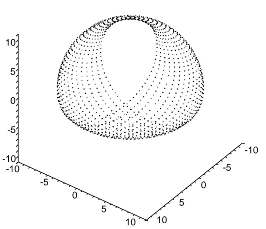
r(x, y) =µ cos(y) cosh(x), sin(y) cosh(x), x − tanh x ¶ . (1.21)

This surface is known as the Beltrami pseudosphere [18], [100]. A plot is given in fig. (1.1). Now it is possible to obtain a ladder of pseudospherical surfaces and correspond-ing solutions of sine Gordon equation through the B¨acklund transformations. It is simpler to work in curvature coordinates; the B¨acklund transformations now read:

∂ ∂x µ ω′ _{− ω} 2 ¶ = 1 sin(θ) µ sinµ ω′ 2 ¶ cos³ω 2 ´ − cos(θ) cosµ ω′ 2 ¶ sin³ω 2 ´¶ (1.22)

(14)

13 1.1 An overview of the classical treatment of surface transformations. ∂ ∂y µ ω′_{− ω} 2 ¶ = 1 sin(θ) µ cosµ ω′ 2 ¶ sin³ω 2 ´ − cos(θ) sinµ ω₂′ ¶ cos³ω 2 ´¶ (1.23)

where I recall that θ is the angle at which the tangent planes of the two surface at corresponding points meet. Note that, if one starts with the solution ω = 0, then by a simple integration it is readily obtained

ω′(x, y) = 4 arctan³ex−y cos(θ)sin(θ)

´

, (1.24)

that corresponds to (1.20) for θ = π

2 (that is in the case of Bianchi transformations).

To this solution one can verify that it corresponds a little modification of the Beltrami pseudosphere, that is the surface:

r(x, y) = µ

sin(θ) cos(y)

cosh(X), sin(θ)

sin(y)

cosh(X), sin(θ) (X − tanh X) + y cos(θ) ¶

, (1.25)

where X = x−y cos(θ)_sin(θ) . In terms of the variables (X, y) it appears very similar to the surface of revolution (1.21). Indeed it is obtained by a rotation of the same curve that gives (1.21) plus a translation parallel to the same axis (the z-axis) in such a way that the ratio of the velocity of translation to that of rotation is a constant (given by cos(θ)). The surfaces obtained with this type of roto-translations are called helicoids [18]. Now it is possible to compose two solutions (1.24) and then use the B¨acklund transformations in the form (1.10) to obtain the corresponding pseudospherical surface. Let me use the parameters θ1 and θ2

       ω1 = 4 arctan µ

ex−y cos(θ1)sin(θ1)

¶

= 4 arctan¡eX1¢ ,

ω2 = 4 arctan

µ

ex−y cos(θ2)sin(θ2)

¶

= 4 arctan¡eX2¢ .

(1.26)

The composition of these two solutions, using the permutability theorem (1.13), gives:

ω12= 4 arctan Ã sin¡_θ₁_+θ₂ 2 ¢ sin¡_θ₁_−θ₂ 2 ¢ sinh¡_X₁_−X₂ 2 ¢ cosh¡_X₁_+X₂ 2 ¢ ! .

Corresponding to ω1 and ω2 one has the two surfaces:

       r1 = µ sin(θ1) cos(y) cosh(X1) , sin(y) cosh(X1)

, sin(θ1) (X1− tanh X1) + y cos(θ1)

¶ r2 = µ sin(θ2) cos(y) cosh(X2) , sin(y) cosh(X2)

, sin(θ1) (X2− tanh X2) + y cos(θ2)

(15)

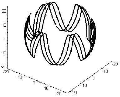
Figure 1.2: The two-soliton pseudospherical surface with θ1 = π₄ and θ2 = π₂

In curvature coordinates the transformations (1.10) between r′ _{and r is given by [18]:}

r′ = r + sin(θ) Ã cos¡ω′ 2 ¢ cos¡_ω 2 ¢ ∂r ∂x − sin¡ω′ 2 ¢ sin¡_ω 2 ¢ ∂r ∂y ! . (1.28)

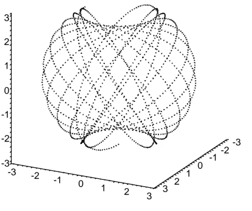
At this point there are all the elements to write down the explicit family of surfaces corresponding to the two-soliton solution ω12; by (1.28) it follows that:

r12=r1+ sin(θ2) Ã cos¡_ω₁₂ 2 ¢ cos¡ω1 2 ¢ ∂r1 ∂x − sin¡_ω₁₂ 2 ¢ sin¡ω1 2 ¢ ∂r1 ∂y ! = =r2+ sin(θ1) Ã cos¡ω12 2 ¢ cos¡_ω₂ 2 ¢ ∂r2 ∂x − sin¡ω12 2 ¢ sin¡_ω₂ 2 ¢ ∂r2 ∂y ! . (1.29)

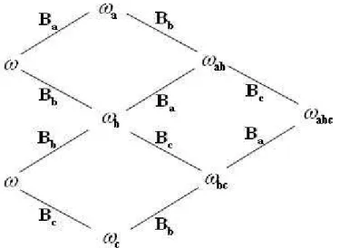
A plot of a particular example of such surfaces is given in figure (1.2). The implication of the permutability theorem are noteworthy also by the point of view of dynamical systems. By its iteration it is in fact possible to construct N -soliton solutions (a non linear superposition of N single soliton solutions) of the sine Gordon equation with a purely algebraic procedure. The procedure can be represented in a diagram known as

(16)

15 1.2 The Clairin method

Figure 1.3: A Bianchi lattice

the Bianchi lattice (see figure (1.3)). As we will mention later, just a rediscovery of the permutability theorem in some physical applications allowed to rescue the subject of B¨acklund transformations in the second part of the twentieth century after the neglect in which it fell after the World War I. By the my point of view, the very deep coupling between algebraic and analytic results on solutions of non linear evolution equations on one hand and the geometry of surfaces on the other has been underestimated until today; yet the usefulness, that I hope will emerge also from this work, of the B¨acklund transformations in the theory of dynamical systems, but also as a tool for solving, nu-merically or analytically, systems of evolution equations, legitimates a broader interest in the geometrical aspects of such transformations.

1.2 The Clairin method

In 1903 Jean Clairin gave important contributions [29] to the subject of B¨acklund transformations. His results were broadly used in the 1970s. He had in mind to extend analytically the results of Bianchi to the case of a generic partial differential equation of second order. Although the Clairin approach is analytic and direct, often it requires tedious calculations. For completeness I will illustrate the method first with a simple generic situation and then getting again the B¨acklund transformations for the sine Gordon equation with an application of the method.

Suppose to have a generic partial differential equation of second order in two indepen-dent variables: F (α, β, ω,∂ω ∂α, ∂ω ∂β, ∂2_ω ∂α2, ∂2_ω ∂α∂β, ∂2_ω ∂β2) = 0. (1.30)

(17)

Following Clairin [29], for simplicity of notation I pose:

p = ∂ω ∂α, q = ∂ω ∂β, r = ∂2_ω ∂α2, s = ∂2_ω ∂α∂β, t = ∂2_ω ∂β2.

The notations for the transformed variables are the same, so ˜p = ∂ω˜

∂α and so on. Clairin

assumed that the first derivatives of ω are connected by the following system: p = f (ω, ˜ω, ˜p, ˜q),

q = g(ω, ˜ω, ˜p, ˜q). (1.31) The compatibility of this system requires

∂p ∂β =

∂q ∂α.

If this integrability condition is identically satisfied by equation (1.30) for the variable ˜

ω, then the equations (1.31) are the B¨acklund transformations for (1.30). In fact, if one has a solution of (1.30), then the system (1.31) provides a new solution of the same equation by solving the resulting first order differential equations. At this point it is important to stress that, as noted by Forsyth [39] (see also [69]), when f and g in (1.31) are independent of ˜ω, then the compatibility equation, in some particular cases, can be seen as a Lie contact transformation. More specifically, when ˜ω is absent, ∂p_∂β₋_∂α∂q = 0 can be rewritten as:

∂f ∂ωg − ∂g ∂ωf + µ ∂f ∂ ˜p − ∂g ∂ ˜q ¶ ˜ s + ∂f ∂ ˜qt −˜ ∂g ∂ ˜p˜r = 0. (1.32) In order to satisfy this integrability condition, one can distinguish between two possi-bilities: or it is satisfied identically, so that the coefficient of ˜s, ˜r and ˜t are zero and (1.32) can be transformed in a contact transformation [39]:

d˜_{ω − ˜pdα − ˜qdβ = µ(dω − pdα − qdβ),}

or the integrability condition can be satisfied because ˜ω is a solution of the partial differential equation (1.32): in this case one has a B¨acklund transformation. In order to clarify how practically works the method, consider again the sine Gordon equation:

∂2_ω_˜

∂αβ = sin(˜ω).

For the sake of simplicity let me take equations (1.31) of the form: q = c(˜ω)˜q + µ(ω, ˜ω),

(18)

If the general form (1.31) for p and q is retained, one needs of a huger analysis but reaches the result given by (1.33). For more details see [6]. The compatibility condition (1.32) now reads: µ dc d˜ω − dh d˜ω ¶ ˜ q ˜_{p + (c − h) sin(˜ω) +} ∂µ ∂ωp + ∂µ ∂ ˜ωp −˜ ∂m ∂ωq − ∂m ∂ ˜ωq = 0.˜ (1.34) Using (1.33), this relation becomes:

µ dc d˜ω − dh d˜ω ¶ ˜ q ˜_{p+(c−h) sin(˜ω)+}µ ∂µ ∂ωd + ∂µ ∂ ˜ω ¶ ˜ p−µ ∂m_∂ωc +∂m ∂ ˜ω ¶ ˜ q+∂µ ∂ωm− ∂m ∂ωµ = 0. (1.35) Differentiating with respect to ˜p and ˜q one sees that:

d

d˜ω(c − d) = 0.

Let me pose c = −1 and h = 1. Differentiating (1.35) with respect to ˜p with these constraints one obtains:

∂µ ∂ω +

∂µ

∂ ˜ω = 0 =⇒ µ = µ(ω − ˜ω), while, differentiating with respect to ˜q

m = m(ω + ˜ω).

Inserting this forms in (1.35), one is left with the functional differential equation:

−2 sin(˜ω) + ∂µ(ω − ˜ω)_∂ω m(ω + ˜_{ω) −} ∂m(ω + ˜ω)

∂ω µ(ω − ˜ω) = 0. In order to solve this equation, let me differentiate with respect to ω, getting:

∂2_µ_(ω−˜_ω) ∂ω2 µ(ω − ˜ω) = ∂2_m(ω+˜_ω) ∂ω2 m(ω + ˜ω).

The r.h.s. of this equation is a function of ω + ˜_{ω while the l.h.s. a function of ω − ˜ω, so} both sides must be equal to the same constant. Because in the functional differential equation a trigonometric function appears, this constant can be assumed real and negative, say −K2_{. So:}

µ = A cos (K(ω − ˜ω)) + B sin (K(ω − ˜ω)) , m = C cos (K(ω + ˜ω)) + D sin (K(ω + ˜ω)) .

(19)

18 1.3 The Renaissance of B¨acklund transformations

Substituting this forms in the functional differential equation and evaluating all at ω = 0, one finds the constraints 2K = 1, AD = BC, AC + BD = 4. The B¨acklund transformations for the sine Gordon equation are attained by posing A = C = 0,

D 2 =

2

B = a. In this case the transformations (1.33) read:

q + ˜q 2 = 1 asin µ ω − ˜ω 2 ¶ , p − ˜p 2 = a sin µ ω + ˜ω 2 ¶ ,

that are exactly the relations (1.8) and (1.9). After the revival of the subject of Bäcklund transformations in the last half of the twentieth century, the construction of such transformations for a number of equations of physical interest (for example KdV, mKdV, NLS, Ernst equation) was obtained just using the Clairin method [6], [69], [66]. A last observation on the terminology usually found in the literature: commonly the transformation that links solutions of the same differential equation is called an auto-Bäcklund transformation, in opposition to the case of transformation linking solutions of two different differential equations: generally speaking this last one is the Bäcklund transformation. Since in this work I will deal only with auto-Bäcklund transformations, I will speak simply of Bäcklund transformations and no confusion can arise.

1.3 The Renaissance of B¨

acklund transformations

After a nearly silent period in the scientific community on the subject, in 1953 the B¨acklund transformations and soliton theory took a new run to establish themselves in physics. About fifteen years before, Frenkel and Kontorova, in order to explain the mechanism of plastic deformations in the crystal lattice of the metals, introduced [40] a lattice dynamic model describing how many atoms can form long dislocation line. If qn

is the distance of the n-th atom from its equilibrium position, a is the lattice constant and A and B two constants, then the equations of motion for the qn’s are:

md 2_q n dt2 = −2πA sin ³ 2πqn a ´ + B (qn+1− 2qn+ qn₋₁)

This is clearly the spatial discrete version of the sine Gordon equation: in fact in the continuous limit, with a suitable change of the variables, the equation can be put in the form φtt− φxx+ sin(φ) = 0 and in turn this equation, with the changes 2α = x + t and

2β = x−t takes the usual form φαβ = sin(φ). More than ten years after the publication

of Frenkel and Kontorova results, Alfred Seeger, while working on his Phd thesis, became aware by chance of the works of Bianchi on sine Gordon equation. So a number of well known solitonic features, such as the preservation of shape and velocity after

(20)

19 1.3 The Renaissance of B¨acklund transformations

collisions, were obtained [104] by means of the permutability theorem. In 1967 Lamb [67] derived the sine Gordon equation as a model for optical pulse propagation in a two energy level medium having relaxation times which are long compared to pulse length (ultrashort optical pulses). Lamb was aware of the Seeger works, so in 1971 [68] he used the permutabilty theorem to analyse the decomposition, experimentally observed, of “2N π” pulses into N stable “2π” pulses. The situation became even more interesting after the work of Wahlquist and Estabrook [122] on B¨acklund transformations for the KdV equation of the 1973. In fact not only they found the transformations and the associated permutability theorem for the KdV equation, but moreover they stressed how an iteration of this theorem can analytically describe the behavior of the soliton solutions numerically observed by Zabusky and Kruskal in 1965 [131]. Furthermore a connection with the incoming Inverse Spectral Transform theory was established. Let me summarize their findings.

They rewrote the KdV equation:

ut+ (6u2+ uxx)x = 0

by introducing the potential function defined by u = −wx. This potential function

satisfies the equation:

wt= 6wx2− wxxx,

Given a solution u of the KdV and then the associated potential w, another solution u1 with potential w1 can be found by the following B¨acklund transformations:

(w1+ w)x= (w1 − w)2− λ1

(w1+ w)t= 4¡λ1u1+ u2− u(w1− w)2− ux(w1− w)

¢ (1.36) where λ1 is an arbitrary parameter. The permutability theorem allowed them to find

a relation between the elements of a soliton ladder. In particular by considering sub-sequent transformations induced by (1.36) with different parameters, for example the transformation from u to u1 with λ1 and then from u1 to u12 with parameter λ2, they

expressed the nth step of the ladder by the recursion relation:

wn = wn₋₂+

λn− λn₋₁

w_(n−1)′ − wn₋₁

(1.37)

where the subscript n denotes the set of n parameters {λ1, . . . λn} and n′ the set

{λ1, . . . λn₋₁, λn+1} (with w0 = w). So for n = 3 one has:

w123 = w +

λ2 3− λ22

w13− w12

,

that can be obviously expressed in terms of only single soliton solutions by an iteration of the formula (1.37) in the case n = 2. Note that the first of the equations (1.36) has

(21)

20 1.4 B¨acklund transformations and the Lax formalism

the form of a Riccati equation: in fact, by posing v = w1− w, one has:

vx+ 2u = v2− λ1.

The linearization of this equation by the substitution v = −ψx

ψ gives:

ψxx+ (2u − λ)ψ = 0,

that is the Schrödinger equation: this result gave the connection between the Bäck-lund transformation of the KdV and the outstanding observation by Gardner, Green, Kruskal and Miura [42] that the solutions of the KdV equation itself are related with the potential of the Schrödinger equation. In 1974, one years after the work of Wahlquist and Estabrook, Lamb [69], by applying the Clairin method, found the Bäcklund trans-formations for the NLS equation. Again a permutability theorem was obtained (al-though, in the words of Lamb [69] “the result appears to be too complex to be useful for computational purposes”) and a connection with the linear equations for the inverse problem associated with the NLS equation was established. From now on a lot of results on Bäcklund transformations for many classes of integrable partial differential equations were obtained; for a review see [101]. At this point it was clear that there are some characteristic properties common to all integrable equations: they possess a Lax representation, which we will analyze later, are solvable by inverse scattering transform and possess Bäcklund transformations. Nevertheless, as noted first by Wojciechowski in 1982 [126], although many finite dimensional systems also admit Lax representa-tion and are completely integrable, the analogue of Bäcklund transformarepresenta-tions for these systems was not known. So in his aforementioned work he provided the Bäcklund transformations for the classical Calogero-Moser system. There he clearly noticed how the Bäcklund transformations for finite dimensional system can be seen as canonical transformations preserving the algebraic form of the Hamiltonian. Really this is not an accident as it will be clarified in 1.5.

1.4 B¨

acklund transformations and the Lax

formal-ism

The Renaissance of B¨acklund transformations matches with the golden age of the integrability theory and of the associated inverse spectral methods. As it is well known, in the later sixties fundamental developments were obtained in the theory of nonlinear differential equations. On the one hand in [42] were derived explicit solutions of the KdV equation and was described the interaction of an arbitrary number of solitons, on the other hand Peter Lax in [71] introduced an operatorial compatibility condition that subsequently allowed to extend the method adopted in [42] to solve a number of

(22)

nonlinear evolution equations with ubiquitous physical applications. Let me summarize the mean features of the Lax method in order to well understand the connections with the B¨acklund transformations theory. The prototypical example of Lax pair is the one that generates the KdV equation. One introduces two linear problems associated to two operators L and M as follows:

Lφ = λφ, L = ∂_x2+ u(x, t), (1.38a)

φt= M φ, M = γ − 3ux− 6u∂x− 4∂xxx. (1.38b)

Here λ is the spectral parameter and γ is an arbitrary constant. The function φ, that according to (1.38a) can be reads as a wave function for the Schr¨odinger equation with potential u(x, t), depends on x, t and λ. The compatibility equations for the wave function φ lead to the Lax equation:

Lt+ LM − ML = Lt+ [L, M ] = 0 (1.39)

and this in turns is equivalent to the KdV equation. The core of the inverse spectral method, the spectral analysis, is derived from the study of equation (1.38a). The physical interpretation of the method is well described by Fokas; by using his words [38]:“Let KdV describe the propagation of a water wave and suppose that this wave is frozen at a given instant of time. By bombarding this water wave with quantum particles, one can reconstruct its shape from knowledge of how these particle scatter. In other words, the scattering data provide an alternative description of the wave at a fixed time”. Once the scattering data have been found, it is possible to compute their time dependence thanks to (1.38b), and so insert the time dependence in the solution of the KdV. More precisely, given u(x, 0), the spectrum of the Schr¨odinger equation (1.38a) is given by a finite number of discrete eigenvalues, say λ = {κ2

n}Nn=1 for λ > 0

and a continuum set, λ = −k2_{, for λ < 0. The asymptotics of the corresponding}

eigenvectors (at t = 0) can be written as follows:

λ > 0; _{x → −∞} φn(x, 0, κn) ∼ cn(0)e−κnx with

Z +∞

−∞

φ2_n(x, 0, κn)dx = 1;

λ < 0; _{x → −∞} _{φ(x, 0, k) ∼ T (k, 0)e}−ikx, x → +∞ φ(x, 0, k) ∼ e−ikx+ R(k, t)eikx,

where T (k, t) and R(k, t) are the transmission and reflection function for the wave function φ. The time evolution of these functions and of cn(t) can be found by equation

(1.38b); the result is cn(t) = cn(0)e4κ

3

nt, T (k, t) = T (k, 0) and R(k, t) = R(k, 0)e8ik3t.

At this point the scattering data are completely described by the set:

(23)

The link between the corresponding solution of the KdV and this data set is given by a linear integral equation; indeed if one defines the function F (x, t) by:

F (x, t) = N X n=1 c2n(t)e−κn x + 1 2π Z ∞ −∞ R(k, t)eikxdk,

then it solves the Gel’fand-Levitan-Marchenko equation:

K(x, y, t) + F (x + y, t) + Z ∞

x

K(x, s, t)F (s + y, t)ds = 0

and the function u(x, t) is reconstructed by:

u(x, t) = 2 ∂

∂xK(x, x, t).

Now the connection with B¨acklund transformations. Suppose to have two different solutions, u and ˜u, to the KdV equation. Correspondingly to these solutions there must exist two different spectral problems, the first given by the equations (1.38a) and (1.38b), and the other by:

˜

L ˜φ = λ ˜φ, L = ∂˜ _x2+ ˜u(x, t), (1.40a) ˜

φt= ˜M ˜φ, M = γ − 3˜u˜ x− 6˜u∂x− 4∂xxx. (1.40b)

Suppose also that u and ˜u are linked by a B¨acklund transformation. The relation between the two solutions defined by this transformation reflects into a relation between the wave functions of the two spectral problems. This means that it has to exist an operator D, that we will call the dressing operator or dressing matrix and that depends on u, ˜u and λ, such that

˜

φ = Dφ. (1.41)

Inserting this equation in (1.40a) and taking into account (1.38a), one obtains the equation for the B¨acklund transformations in the Lax formalism:

˜

LD = DL (1.42)

As we will see, this boxed equation will be of fundamental importance for the core of this work. Obviously, given a dressing operator D fulfilling (1.42), one has to ensure also that (1.40b) is fulfilled. For differential equations possessing a Lax representation, the problem of finding B¨acklund transformations reduces to the problem of finding the corresponding dressing operator.

(24)

23 1.5 B¨acklund transformations and integrable discretizations

1.5 B¨

acklund transformations and integrable

dis-cretizations

1.5.1 Integrable discretizations

Cellular automata, neural networks and self-organizing phenomena are only few of the key notions appearing in the modern developments of discrete dynamics. One of the main practical interest in integrable discretizations of nonlinear evolution equations arises from the needs of computational physics. The problem is to construct a discrete analogue of the continuum model preserving its mean features. In statistical mechanics, for obvious reasons, it is of fundamental importance that the long-term dynamics of the continuous model can be related to the corresponding dynamics of the discrete system. An encyclopedic work on the Hamiltonian approach to integrable discretization is that of Suris [115]. As a matter of fact the problem of integrable discretizations is not to solve the discrete dynamics, but rather to find what is the most appropriate discrete counterpart of a continuous system. Since in this work we will deal only with integrable system, for the sake of completeness I will first recall the Liouville-Arnold theorem on complete integrable systems and then I will specify, following Suris, what is meant by “appropriate” discretization.

Theorem 1 Suppose to have an autonomous Hamiltonian system (with Hamiltonian H) with n degree of freedom (the dimension of phase space is then 2n) and with n independent first integrals in involution, that is n functions Ik, k = 1 . . . n, such that

the gradients ∇Ik are n independent vectors for every point of the phase space and the

Poisson bracket {Ik, Im} vanishes for every k, m = 1 . . . n. Consider the level set

Ma = {x ∈ R2n : Ik= ak, k = 1 . . . n},

where a ∈ Rn_{. Then:}

• Ma is a smooth manifold invariant under the phase flow associated with I1, . . . In;

• If Ma is compact and connected it is diffeomorphic to an n-dimensional torus,

that is the set Tn _{of n angular coordinates:}

Tn _{= {φ}1, . . . φn};

• The flow with respect to H determines a quasi-periodic motion on Ma:

dφi

(25)

• The equations of motion with respect the Hamiltonian H can be integrated by quadratures.

For the detailed proof of these statements the reader can see for example [8].

Now, having in mind the precise formulation of Suris [115], we can state the problem of integrable discretization as in the following. Suppose to have an autonomous complete integrable system, governed by an Hamiltonian H, and denote simply by x the dynamic variables of this system. Let Ik(x) be the integrals in involution. The equations of

motion will be given by:

˙x = {H, x} = f(x). (1.43) The “appropriate” discrete counterpart of this system will be a family of maps:

˜

x = Φ(x, µ)

depending smoothly on a parameter µ and such that:

• In the limit µ → 0 the map approximate the flow (1.43): Φ(x, µ) = x + µf (x) + O(µ2).

• The map is Poisson with respect to the bracket {·, ·} or some its deformation {·, ·}µ= {·, ·} + O(µ).

• The map is integrable and the integrals approximate those of the continuous system: Ik(x, µ) = Ik(x) + O(µ).

Note that it is not requested the explicitness of the map, nor the conservation of the orbits.

If the more restrictive conditions {·, ·}µ = {·, ·} and Ik(x, µ) = Ik(x) are fulfilled, than

I will talk about exact-time discretization: as will be showed in the chapter (4), at least in some special cases of such discretization for the Kirchhoff top, and as a conjecture for the exact time discretization of the Kirchhoff top as a whole, it will be possible to preserve also the physical orbits of the system.

A number of methods have been proposed in the course of time to establish a modus operandi in discretizing continuous flows. A complete list can be found in [115] (see also [116]); some of these approaches are:

• The Ablowitz-Ladik approach [1], [2]: if an integrable system can be written as the compatibility condition for two associated linear problem, then the corre-sponding discrete system can be found by discretizing, in some way, one or both of them. “In some way” indeed means that this can be done in various ways;

(26)

Faddeev and Takhtajan [35] try to get some fixed rule by focusing on Hamilto-nian properties of the model considered: a common feature for models in 1 + 1 dimensions is to retain the r-matrix and substitute the linear Poisson bracket with the quadratic one (see appendix B for a discussion on linear and quadratic r-matrix structures).

• The Hirota method: it is based on the bilinear approach introduced by Hirota [51] and widely used to obtain soliton solutions of non linear evolution equations. It seems to have some connections with a method proposed by Kahan but that has remained largely ignored [87]. As noted in [115], the mechanism behind the method is yet to be fully understood.

• The Moser and Veselov approach [78], [129], [127]: it is based on discrete la-grangian equations obtained by means of variational principles. It is also known as the factorization method and is indeed based on some observations of Symes [119] on the connection of Toda flow with the QR-algorithm, an important tool in the numerical analysis for the diagonalization of matrices. Moser and Veselov works gave rise to a widespread and renewed interest in the theory of integrable maps within the mathematical physics community.

• Geometric method [118], [23], [26]: as we have seen in the first part of this work, there is a deep connection between geometry of surfaces and integrable differential equations. It is natural then to check what is obtained by discretizing the notions and methods of smooth surface theory. In my opinion this could be one of the more fruitful direction of the future research.

• The B¨acklund transformations method: the approach that represents the ob-ject of the thesis and that will be extensively explained in the next paragraph. In my perspective this is the most satisfactory and efficient method to obtain discrete version of integrable non linear evolution equations that admit a Lax representation; the deep connection with the geometry of surfaces should not be underestimated as a source of new discoveries and new queries.

1.5.2 The approach `

a la B¨

acklund

Quite remarkably, Bäcklund transformations provide a powerful tool in the discretiza-tion of integrable differential equadiscretiza-tions. The idea behind this technique is very simple: suppose that a differential equation possesses an associated Lax structure and a Bäck-lund transformation. By viewing the new solution as the old one but computed at the next time-step, then the Bäcklund transformation becomes a differential-difference (or only difference) equation. The same argument can be repeated also at the level of the Lax matrices, so that one is often able to obtain also the Lax pair for the discrete

(27)

system, showing in this way its integrability. To the best of my knowledge, one of the first clear evidences of the capability of this point of view was given by Levi and Benguria in [72], where these lines of reasoning were used to show that the following differential difference approximation of the KdV equation:

(w(n + 1, t) + w(n, t))_t_{+ [w(n + 1, t) − w(n, t)]} ·

h + 1

2(w(n + 1, t) − w(n, t)) ¸

is indeed integrable. However, in my opinion, in the course of all the eighties the full potential of the Bäcklund transformations was not well understood. As yet mentioned in 1.3, in 1982 Wojciechowski [126] sought to find the analogues of the Bäcklund trans-formations for finite dimensional systems. As a matter of fact he found the Bäcklund transformations for a well known many body system, the so called Calogero-Moser system [27], [77]. His results are noteworthy, but they were forgotten for some time. Furthermore I’m quite sure that Wojciechowski wasn’t aware of Levi and Benguria’s work: in fact only in 1996 it was realized by Nijhoff, Ragnisco and Kuznetsov [84] that indeed the discrete Calogero-Moser model can be inferred from the Bäcklund transformations given in [126]. Let me summarize for completeness the results of Wo-jciechowski. He considered a set of systems of N interacting particles on a line with the following two-body potentials:

           a) V (x) = ℘(x), b) V (x) = 1 x2,¡coth 2_{(x), cot}2_{(x)¢ ,} c) V (x) = 1 x2 + w 2_x2_. (1.44)

where ℘(x) is the Weierstraß elliptic function. The B¨acklund transformations for these systems are given by the following expressions:

˙xk = 2 M X j_6=k ψ(xk− xj) − 2 N X j=1 ψ(xk− yj) + 2λ − wxk ˙ym = 2 M X j=1 ψ(ym− xj) − 2 N X j6=m ψ(ym− yj) + 2λ − wym (1.45)

where k = 1 . . . M , m = 1 . . . N and correspondingly to the case a), b) and c), the function ψ takes the following values:

           a) ψ(x) = ζ(x), M = N, w = 0, b) ψ(x) = 1

x, (coth(x), cot(x)) , M, N arbitrary, w = 0, c) ψ(x) = 1

x, M, N arbitrary, w 6= 0.

(28)

Here ζ(x) is the Weierstraß zeta function. Wojciechowski was able to show that indeed the conditions of compatibility reduce to the dynamical equations and that the trans-formations provide an algebraic construction of new solutions thanks to a permutabilty theorem. Furthermore the transformations (1.45) are canonical because there exist a generating function F such that ˙xk = _∂x∂F

k and ˙yk = −

∂F

∂yk. This canonical

transforma-tion has also the property to preserve the algebraic form of the Hamiltonian (obviously other than the Hamiltonian character of the equations of motion). For a twist of fate the work of Wojciechowski was recognized in 1996 to discretize the corresponding con-tinuous flow in [84], a work which proposed the discretization of a relativistic variant of the Calogero-Moser model, the so called Ruijsenaars-Schneider model, with transforma-tions that only after, in [64], was recognized to be indeed the Bäcklund transformatransforma-tions for such model. As for the discretization of partial differential equations by means of Bäcklund transformations, the situation was quite similar: in fact some results appear in 1982 [81] and 1983 [83] but only later the relevance of Bäcklund transformations and permutabilty theorems in discretizing PDEs were fully acknowledged [26][82]. So in 1983 Nijhoff, Quispel and Capel [83] found a difference-difference version of some nonlinear PDEs of physical interest in 1+1 dimension. Among them there was the KdV equation. Unlike Wojciechowski now the authors were aware of the work of Levi and Benguria so that they could establish quite clearly (although, it seems, by following an independent way) the connection of their discretization with the Bäcklund transfor-mations and the Bianchi permutability theorem. So if un,m represents the dynamical

variable at site (n, m), where n, m ∈ Z, the lattice version of the KdV reads (see also [82]):

(p − q + un,m+1− un+1,m) (p + q − un+1,m+1+ un,m) = p2 − q2 (1.47)

where p, q ∈ C are two parameters. As shown in [83], this is equivalent to the Bianchi permutability theorem: by combining two B¨acklund transformations for the KdV, as given in [81], the first, say ˜u, with parameter p and the second one, say ˆu, with parameter q, then one obtains the formula:

³

p + q − ˆ˜u + u´(p − q + ˆu − ˜u) = p2− q2

which is equivalent to the lattice KdV equation (1.47): so as stated clearly in [82], the iteration of B¨acklund transformations leads to a lattice of transformed fields u and the Bianchi permutabilty theorem is nothing but consistency condition on the lattice for the partial difference equation.

In the course of 1990s, in the wake of Veselov works on Lagrange correspondences [127], [128], [129], that is multi-valued symplectic maps that have enough integrals of motion and that are time discretizations of some known classical Liouville integrable systems, a lot of results on discretization of finite dimensional integrable systems were achieved: for the Ruijsenaars-Schneider model [84], the Henon-Heiles, Garnier and Neumann systems [91], [92], [53], the Euler top [24], the Lagrange top [25], the rational Gaudin

(29)

magnet [52] and others (see also the excellent book by Suris [115] and the references therein). It turned out [65] that almost all the discretizations for these systems associate new solutions to a given one: it was clear then that they are Bäcklund transformations for such systems. These developments suggested to Sklyanin and Kuznetsov that the concept of Bäcklund transformations could be revised in order to highlight some new aspects. Actually in the previous times these two authors were very active in the field of separation of variables and its connection with the new techniques of classical and quantum inverse scattering method, so not only they were able to clearly elucidate the role of Bäcklund transformations in the context of finite dimensional integrable systems, but they also established deep and fruitful connections with Hamiltonian dynamics and separation of variables. I think that all the potentialities of these new ideas are not yet fully exploited, and I hope to give in this work some new light on the geometric, mechanical and Hamiltonian meaning of Bäcklund transformations for finite dimensional systems. The fundamental paper that now I will survey is [64] (see also [65]). For a more detailed account on the links between the inverse scattering method and the classical notion of separation of variables the reader can see [109]. Suppose to have a classical integrable dynamical system described by a Lax matrix L(λ), where λ is the spectral parameter, and that the commuting Hamiltonians Hi can

be obtained by the coefficients of the characteristic polynomial det(L(λ) − γ1). Let the dynamical variables be qi and pi, i = 1 . . . N , and assume for simplicity that these

variables are canonical:

{qi, qj} = 0, {pi, pj} = 0, {qi, pj} = δij.

Correspondingly to the matrix L(λ) it has to exist the Lax matrix ˜L(λ) of the trans-formed variables, that is ˜L(λ) = L(λ, ˜. q, ˜p). As repeatedly noticed [37] [126], [102], [127], [65], [84], [78], [75] [4] [110], [111], [36] the B¨acklund transformations can be seen as canonical transformations preserving the algebraic form of the Hamiltonians. Since the characteristic polynomial is the generating function of the integrals of motion, their invariance amounts to require the existence of a similarity matrix, the dressing matrix, that intertwines the two Lax matrices (see also (1.42)):

˜

L(λ)D(λ) = D(λ)L(λ). (1.48) Obviously the matrix D(λ) needs not to be unique because a dynamical system can have different Bäcklund transformations. More remarkably it is possible to have one-parametric or multi-one-parametric families of Bäcklund transformations: as we will see this is related to the existence of a dressing matrix D(λ) such that det(D(µ)) = 0, where µ is a particular (but arbitrary) value of the spectral parameter λ; it is not an overstatement to say that this fact is at the core of the Sklyanin and Kuznetsov speculations: indeed it allows them also to introduce a new property of Bäcklund transformations, that is the spectrality. But let me go with order.

(30)

Let me assume to be in the simplest nontrivial case, namely the case of 2 × 2 matrices. Assume also that it is possible to find a parametrization of the matrix D(λ) such that its determinant is zero when λ = µ. This means that D(µ) is a rank one matrix. Let |Ω(µ)i be the corresponding kernel. By acting with it on the equation (1.48), one finds:

˜

L(µ)D(µ)|Ω(µ)i = 0 ⇒ D(µ) (L(µ)|Ω(µ)i) = 0.

But this implies that the vector L(µ)|Ω(µ)i is proportional to the kernel |Ω(µ)i, that is:

L(µ)|Ω(µ)i = γ(µ)|Ω(µ)i

and, in turns, this means just that |Ω(µ)i is also the eigenvector, often called the Baker-Akhiezer function, of L(µ) with eigenvalue γ(µ), so that the characteristic polynomial evaluated at λ = µ is zero:

det(L(µ) − γ1) = 0. (1.49) This seems to be an harmless equivalence but actually it is the separation equation, in the sense of Hamilton Jacobi separability, for the dynamical system. Let me explain this point. The eigenvalue |Ω(µ)i is defined up to a multiplicative factor, so it is possible to define a normalization for it. Fix this normalization by introducing the vector |α(µ)i:

hα(µ)|Ω(µ)i = 1.

In general the vector |α(µ)i can depend also on the dynamical variables. With the above normalization |Ω(µ)i becomes a meromorphic function on the surface defined by det(L(µ) − γ(µ)1) = 0 (obviously to any fixed µ there correspond 2 possible values of γ(µ) for a 2 × 2 Lax matrix). At this point there is the crucial observation: the poles of the eigenvector |Ω(µ)i, say at µ = xj can be explicitated and Poisson commute, the

corresponding eigenvalue of L(xj), say γj = γ(xj), or in general functions of γj, together

with the variables xj, are a set of separated canonical variables for the dynamical system

described by the Lax matrix L(λ). This means that: a) the Poisson brackets for xj and γj are canonical:

{xi, xj} = 0, {γi, γj} = 0, {xj, γi} = δij. (1.50)

b) there exist a set of N relations binding together each pair (xj, γj) with the

Hamil-tonians of the system Hi, i = 1 . . . N .

In order to prove the first assertion one needs of the Poisson brackets between the entries of L(λ), and these are usually provided by the r-matrix. For example let me suppose to have the 2 × 2 Lax matrix:

L(λ) = µ A(λ) B(λ) C(λ) −A(λ)

(31)

satisfying the following Poisson brackets (for details on r-matrix formalism see appendix B):

{L(λ) ⊗ 1, 1 ⊗ L(µ)} = [r(λ − µ), L(λ) ⊗ 1 + 1 ⊗ L(µ)] (1.51) where, by definition, {L(λ) ⊗ 1, 1 ⊗ L(µ)} is given by:

{L(λ) ⊗ 1, 1 ⊗ L(µ)}jk,mn = {L(λ)jm, L(µ)kn}

and r(λ) is the classical rational r-matrix, proportional to the permutation operator P in C2_{⊗ C}2_{, defined by [35], [9]:} r(λ) = P λ, P (φ ⊗ ψ) = ψ ⊗ φ, P =     1 0 0 0 0 0 1 0 0 1 0 0 0 0 0 1     .

These Lax and Poisson structures are actually common to a number of integrable systems (see for example[35], [9]) including the rational Gaudin model [52]. The explicit Poisson brackets for the matrix elements A(λ), B(λ) and C(λ), corresponding to (1.51), can be easily computed as:

{A(λ), A(µ)} = {B(λ), B(µ)} = {C(λ), C(µ)} = 0, (1.52) {A(λ), B(µ)} = B(µ) − B(λ) λ − µ , (1.53) {A(λ), C(µ)} = C(λ) − C(µ) λ − µ , (1.54) {B(λ), C(µ)} = 2(A(µ) − A(λ)) λ − µ . (1.55) It turns out [109] that in this case any constant numeric vector of normalization |α(µ)i is able to produce a new set of separated variables. For example if one takes hα| = (1, 0), then the equation for the poles of the Baker-Akhiezer function reads:

hα(xj)|Ω(xj)i = 0.

It is straightforward to see that the compatibility of this equation with the correspond-ing eigenvector relation L(xj)|Ω(xj)i = γ(xj)|Ω(xj)i gives:

B(xj) = 0 γ(xj) = −A(xj)

Now by solving B(xj) with respect to xj, one obtains the first set of commuting

variables. Indeed they commute as a consequence of the second relation in(1.52), {B(λ), B(µ)} = 0, which readily implies the commutativity of the B(µ)’s zeroes:

(32)

{xi, xj} = 0. Equivalently, thanks to the first relation in (1.52), one has the Poisson

commutativity of the variables γj = −A(xj). For the commutation relations between

xi and A(xj) one has to use (1.53). First of all let me find the Poisson bracket between

xj and any function f . By using B(xj) = 0, one clearly has:

{f, B(xj)} = 0 = {f, B(µ)}|_µ=x_j + B′(xj){f, xj} ⇒ {f, xj} = −

{f, B(µ)}|µ=xj

B′_(x_j₎

where in the calculation of the bracket {f, B(µ)} one considers µ as a constant. Then for {A(xi), xj} one has:

{A(xi), xj} = {A(λ), xj}|_λ=x_i + A′(xi){xi, xj} = {A(λ), xj}|_λ=x_i

because {xi, xj} = 0. By putting all together:

{A(xi), xj} = − {A(λ), B(µ)}|λ=xi µ=xj B′_(x_j₎ 1.53 = 1 B′_(x_j₎ B(xi) − B(xj) (xi− xj) .

This relation clearly vanishes for xi 6= xj because B(xi) = B(xj) = 0. For i = j, by

l’Hˆopital’s rule, one readily obtains {A(xi), xj} = δij, in agreement with (1.50).

The second assertion, that is the existence of a set of N relations binding together each pair (xj, γj) with the Hamiltonians of the system, is self-evident: since γ(xj) is an

eigenvalue of L(xj), the pair (xj, γj) satisfies det(L(xj) − γ(xj)1) = 0. This is just a

relation between the canonical coordinates (xj, γj) and the N Hamiltonians Hj (recall

that by hypothesis the Hamiltonians are the coefficients of the characteristic equation): it can be used in the usual Hamilton-Jacobi method in order to separate the variables [8]. If one has N pairs (xj, γj), then the separation is complete (in the previous example

this is the case if B(µ) = 0 has N distinct roots). These observations clarify why (1.49) can be seen as the separation equation of the dynamical system.

The strength and attractiveness of all this construction is that it has an almost clear quantum counterpart [112], [64] [108]. The involutivity of the integrals of motion is replaced by the commutativity of the corresponding quantum operators:

{Hi, Hj} = 0 =⇒ [Hi, Hj] = 0 i, j = 1 . . . N.

The set of classical separated coordinates, {xi, γi}Ni=1 satisfies the set of N separation

equations det(L(xi) − γ(xi)1) = 0. Here a problem of ordering operators arises. In the

separation equations the canonical coordinates and the integrals appear; emphasizing these dependencies, the relations det(L(xi) − γ(xi)1) = 0 can be written in general as:

Φi(xi, γi, H1, . . . HN) = 0, i = 1 . . . N. (1.56)

The commutators between the xj’s and the γj’s are obviously given by:

(33)

Suppose that the ordering in (1.56) is exactly as it appears. Since the operators Hi

commute, they will have a common eigenfunction, say Ψ. Applying these eigenfunction to (1.56), one readily realizes that Ψ satisfies the set of N equations:

Φi(xi, −i~

∂ ∂xi

, h1, . . . hN)Ψ = 0, (1.57)

where hi, i = 1 . . . N are the eigenvalues corresponding to Hi. The eigenfunction Ψ is

then factorized into functions of one variables:

Ψ =

N

Y

j=1

ψi(xi)

each satisfying the differential equation:

Φi(xi, −i~

∂ ∂xi

, h1, . . . hN)ψi(xi) = 0.

It is possible to establish also a connection between Bäcklund transformations and the so-called Baxter’s Q-operator [85], [112]; this operator, that is indeed a family of operators depending on a parameter, say µ, commutes with the Hamiltonians of the system and its eigenvalue solves the Baxter’s equation, that can be considered the quantum counterpart of the separation equation (1.49). Indeed the Baxter equation allows, exactly as in the classical separation of variables, to determine the spectrum of commuting Hamiltonians, reducing the spectral problem to a set of one-dimensional problems. Experience shows [112] that the classical Bäcklund transformations are exactly the similarity transformations induced by the Baxter’s operator. In fact, since the Bäcklund transformations are canonical maps, it is possible to describe them by a generating function: if {qi, pi} are the dynamical variables for our system and {˜qi, ˜pi}

are the B¨acklund transformed variables, then must exist a generating function, say Fµ(q, ˜q) such that: pi = ∂Fµ ∂qi , p˜i = − ∂Fµ ∂ ˜qi

the subscript µ on F denotes the possibility that F can indeed depends on a parameter µ because, as explained before, in general one has a parametric family of B¨acklund transformations. The quantum analog of these canonical transformations is provided by a similarity transformations:

pi = QµqiQ−1µ , p˜i = Qµq˜iQ−1µ .

where Qµ is an integral operator whose kernel, say Kµ, corresponds to the generating

function Fµ through the semiclassical relation:

Kµ ∼ e−(

i ~Fµ).

(34)

In my opinion all these evidences of the connections between the B¨acklund transforma-tions and Baxter’s Q operator need of a profound theoretical setting in order to exploit all the possible implications that can arise from a deeper understanding.

On the account of this brief synopsis on the separation of variables, the means of the spectrality property introduced by Kuznetsov and Sklyanin [64] can be better under-stood. In few words, this property amounts to the following observation [64]: if γ is the variable conjugated to µ:

γ = −∂F_∂µµ, (1.58) then for some function g(γ) one has det(L(µ) − g(γ)1) = 0. Notice that this last equation is just the separation equation (1.49): the canonical conjugation between the variables µj’s and γj’s gives an Hamiltonian interpretation of the relation (1.58). In the

general statement one needs of a function g because, roughly speaking, it is possible that the variables conjugated to the µj’s are some function of the γj’s. As we will

see in the discussion of the discretization of the Gaudin and Kirchhoff models, it is possible to give also another mechanical interpretation of the equation (1.58). Suppose in fact that the B¨acklund transformation is connected to the identity by the parameter µ, so we assume that the map is a smooth function of µ and there exist a value of this parameter, say for simplicity µ = 0, such that

lim

µ→0h(˜q, ˜p) = h(q, p)

for any function h of the dynamical variables. One can now consider the relation defining the map, ˜LD = DL around the point µ = 0; the Taylor series for the matrix D will be D = 1 + µD0 + O(µ2), because it is connected to the identity; by defining

˙L .= lim

µ_→0

˜ L − L

µ , one readily obtains:

˙L = [D0, L],

that is the Lax equation for a continuous flow. Note that D0can depend on a parameter,

so that one has a family of flows. For the Gaudin models and the Kirchhoff top it turns out that this flows are indeed equivalent just to those governed by the Hamiltonian function γ: in this sense, if µ is the evolution parameter (time), the relation between γ and µ is just γ = −∂S

∂µ, where S is the action function [8].

A further remark: the dressing matrix approach to B¨acklund transformations, and then to discretization, is closely related to the factorization method developed by Moser and Veselov in 1991 [78], [127]. The method is based on the following observations: suppose to have a polynomial Lax matrix with a suitable factorization, say L(λ) = A(λ)B(λ), and suppose that by interchanging the two factor matrices one obtains a

(35)

matrix L′_{(λ) belonging to the same polynomial family as L(λ). Then the transformed}

variables appearing in the Lax matrix L′_{(λ) describe the discrete equations of the}

model under consideration. Actually Moser and Veselov generalized a result of Symes on the Toda chain [119]: he showed how the application of the above process to L = exp(K), where K is a symmetric tridiagonal matrix, leads to an integrable mapping which is interpolated by the Toda flow. From my point of view however everything becomes clearer by thinking at the transformation linking L(λ) and L′_{(λ) as a similarity}

transformation; in fact L′_{(λ) = B(λ)A(λ) = A}−1_{(λ)L(λ)A(λ), so that the matrix A(λ)}

represents our dressing matrix and all the considerations of this section can be applied to the factorization method.

At this point we have seen the following features of B¨acklund transformations:

1 They are canonical maps that preserve the algebraic form of the integrals.

2 They can be constructed by means of a similarity transformation with a dressing matrix D. They can depend, in general, by a set of essential parameters {µi}Ni=1.

3 It is possible to parametrize the dressing matrix in such a way that its determinant is zero for an arbitrary value of the spectral parameter, say for λ = µ. Then the B¨acklund transformations will depend on this parameter. Furthermore it is canonically conjugated to γ, where γ is linked to µ by the characteristic curve that appears in the linearization of the integrable system. This is the spectrality property.

4 They discretize a family of flows; the interpolating Hamiltonian can depend on a parameter or a set of parameters: actually it is possible that one can choose their value so to obtain the discretized flow of each of the Hamiltonian Hi of the model.

How we will see, this is the case for the Gaudin models and the Kirchhoff top.

At this list it is possible to add other very significant features that however are conse-quences of the previous ones. That is:

5 Commutativity. Obviously one can compose two B¨acklund transformations with different parameters, say µ1 and µ2. Let me symbolize the transformation with

parameter µ1 with Bµ1 and the one with parameter µ2 with Bµ2. As shown

by Veselov [127], by the property of canonicity and invariance of Hamiltonians follows the commutativity of the transformations: Bµ1Bµ2 = Bµ2Bµ1. In fact,

consider the Poisson map defined by the B¨acklund transformations. If MH is the

manifold of the level set of the integrals:

(36)

then, if it is compact and connected, for the same reason as in the usual Liouville theorem, it must be a torus TN ₌ RN

ZN. Veselov shows that the map determines a

shift on this torus; that is for some function b

φi → φi+ bi(µ), φi ∈ TN.

The commutativity is then obvious. It is also possible to take another perspective to explain the Veselov observation. In fact, if the dynamical variables are {qi, pi}

and the transformed variables are {˜qi, ˜pi}, then, because the transformations are

canonical, the new flows can be written again in Hamiltonian form. Because the generating function of the transformations, say the function F (q, ˜q) such that pi = ∂F_∂q

i and ˜pi = −

∂F

∂q˜i, does not depend on time, there is the equivalence between

the two Hamiltonians: H(q, p) = ˜H(˜q, ˜p); but the B¨acklund transformations preserve also the algebraic form of the integrals, so that also the algebraic form of ˜H(˜q, ˜p) is preserved: this means that (q, p) and (˜q, ˜p) satisfy the same equations of motion but with different initial conditions (by the contrary one has the trivial B¨acklund ˜q = q, ˜p = p by uniqueness theorem on the solutions of ODEs): the two solutions are related by a shift in time. It is clear now that, regarding the transformed variables ˜q and ˜p as algebraic expressions in terms of q and p, they are truly discretization of the dynamical system. A simple example I hope will clarify this point. Let me take an harmonic oscillator with Hamiltonian:

H =X i 1 2(q 2 i + p 2 i).

One can verify that a family of B¨acklund transformations on this system is given by: (˜qi, ˜pi) = Bλ(q, p) = µ qi(1 − λ2) − 2piλ 1 + λ2 , pi(1 − λ2) + 2qiλ 1 + λ2 ¶ . (1.59)

In fact, if (qi(t), pi(t)) is a solution of the equations of motion, so is (˜qi(t), ˜pi(t)).

Obviously for these transformations one has {˜qi, ˜pi} = {qi, pi} and ˜Hi = ˜qi2+ ˜p2i =

q2

i + p2i = Hi. Equations (1.59) define a shift: for example by taking λ = 1, the

value of (˜q, ˜_{p) = (−p}i, qi) is the value of the flow at the time t = π₂. In order to

see this, it suffices to re-parametrize the B¨acklund parameter as λ = tan(t

2). The

transformations now read: ˜

pi = picos(t) + qisin(t),

˜

qi = qicos(t) − pisin(t),

that is the general solution of the equations of motion. These ideas will be further developed in the discussion of the Kirchhoff top.

Backlund transformations and exact time-discretization for Gaudin and related models

Universit´

a degli Studi Roma Tre

Dipartimento di Fisica

via Della Vasca Navale 84, 00146 Roma, Italy

B¨

acklund Transformations and

exact time-discretizations for

Gaudin and related models

Author:

Federico Zullo

Supervisor:

Prof. Orlando Ragnisco

Contents

Chapter 1

Introduction

1.1

An overview of the classical treatment of

sur-face transformations.

1.2

The Clairin method

1.3

The Renaissance of B¨

acklund transformations

1.4

B¨

acklund transformations and the Lax

formal-ism

1.5

B¨

acklund transformations and integrable

dis-cretizations

1.5.1

Integrable discretizations

1.5.2

The approach `

a la B¨

acklund