UNIVERSITY
OF TRENTO
DEPARTMENT OF INFORMATION AND COMMUNICATION TECHNOLOGY
38050 Povo – Trento (Italy), Via Sommarive 14
http://www.dit.unitn.it
S-MATCH: AN ALGORITHM AND AN IMPLEMENTATION
OF SEMANTIC MATCHING
Fausto Giunchiglia, Pavel Shvaiko and Mikalai Yatskevich
February 2004
Technical Report # DIT-04-015
Also: In Proceedings of the European Semantic Web Symposium, LNCS
3053, pp. 61-75, 2004.
S-Match: an algorithm and an implementation of
semantic matching
Fausto Giunchiglia, Pavel Shvaiko, Mikalai Yatskevich
Dept. of Information and Communication Technology University of Trento,
38050 Povo, Trento, Italy
{fausto, pavel, yatskevi}@dit.unitn.it
Abstract. We think of Match as an operator which takes two graph-like
struc-tures (e.g., conceptual hierarchies or ontologies) and produces a mapping be-tween those nodes of the two graphs that correspond semantically to each other. Semantic matching is a novel approach where semantic correspondences are discovered by computing, and returning as a result, the semantic information implicitly or explicitly codified in the labels of nodes and arcs. In this paper we present an algorithm implementing semantic matching, and we discuss its im-plementation within the S-Match system. We also test S-Match against three state of the art matching systems. The results, though preliminary, look promis-ing, in particular for what concerns precision and recall.
1 Introduction
We think of Match as an operator that takes two graph-like structures (e.g., concep-tual hierarchies, database schemas or ontologies) and produces mappings among the nodes of the two graphs that correspond semantically to each other. Match is a critical operator in many well-known application domains, such as schema/ontology integra-tion, data warehouses, and XML message mapping. More recently, new application domains have emerged, such as catalog matching, where the match operator is used to map entries of catalogs among business partners; or web service coordination, where match is used to identify dependencies among data sources.
We concentrate on semantic matching, as introduced in [6], based on the ideas and system described in [2]. The key intuition behind semantic matching is that we should calculate mappings by computing the semantic relations holding between the con-cepts (and not labels!) assigned to nodes. Thus, for instance, two concon-cepts can be equivalent, one can be more general than the other, and so on. We classify all previ-ous approaches under the heading of syntactic matching. These approaches, though implicitly or explicitly exploiting the semantic information codified in graphs, differ substantially from our approach in that, instead of computing semantic relations be-tween nodes, they compute syntactic “similarity” coefficients bebe-tween labels, in the [0,1] range. Some examples of previous solutions are [12], [1], [15], [18], [5], [10]; see [6] for an in depth discussion about syntactic and semantic matching.
In this paper we propose and analyze in detail an algorithm and a system imple-menting semantic matching. Our approach is based on two key notions, the notion of
concept of/at a label, and the notion of concept of/at a node. These two notions
for-malize the set of documents which one would classify under a label and under a node, respectively. We restrict ourselves to trees, and to the use of hierarchies (e.g., ontolo-gies, conceptual hierarchies) for classification purposes. While the classification of documents is undoubtedly the most important application of classification hierarchies, a new set of interesting applications have lately been found out. For instance in [7], classification hierarchies are used to classify nodes, databases and database contents (but in this latter set of applications we need to deal with attributes, a topic not dis-cussed in this paper) in the Semantic Web.
The system we have developed, called S-Match, takes two trees, and for any pair of nodes from the two trees, it computes the strongest semantic relation (see Section 2 for a formal definition) holding between the concepts of the two nodes. The current version of S-Match is a rationalized re-implementation of the CTXmatch system [2] with a few added functionalities. S-Match is schema-based, and, as such, it does not exploit the information encoded in documents. We have compared S-Match with three state of the art schema-based matching systems, namely Cupid [12], COMA [4], and Similarity Flooding (SF) [15] as implemented within the Rondo system [14]. The results, though preliminary, look very promising, in particular for what concerns precision and recall.
The rest of the paper is organized as follows. Section 2 provides, via an example, the basic intuitions behind our algorithm and introduces the notions of concept of/at a label and of concept of/at a node. The algorithm is then articulated in its four macro steps in Section 3, which also provides the pseudo-code for its most relevant parts. Then, Section 4 describes S-Match, a platform implementing semantic matching, while Section 5 presents some preliminary experimental results. Finally, Section 6 provides some conclusions.
2 Semantic Matching
We introduce semantic matching by analyzing how it works on the two concept hier-archies of Figure 1 (a very simplified version of a catalog matching problem).
Fig.1. Two simple concept hierarchies
Preliminary to the definition of semantic matching is the definition of concept
of/at a node, which, in turn, is based on the notion of concept of/at a label. Let us
analyze these two notions in turn, starting from the second.
is-a relation part-of relation
Austria Italy 3 Images Europe 1 2 4
Wine and Cheese
Italy 4 Austria 5 Pictures Europe 2 1 3 A1 A2
The trivial but key observation is that labels in classification hierarchies are used to define the set of documents one would like to classify under the node holding the label. Thus, when we write Images (see the root node of A1 in Figure 1), we do not really mean “images”, but rather “the documents which are (about) images”. Analo-gously, when we write Europe (see the root node of A2 in Figure 1), we mean “the documents which are about Europe”. In other words, a label has an intended meaning, which is what this label means in the world. However, when using labels for classifi-cation purposes, we use them to denote the set of documents which talk about their intended meaning. This consideration allows us to generalize the example definitions of Images and Europe and to define the “concept of/at a label” as “the set of
docu-ments that are about what the label means in the world”.
Two observations. First, while the semantics of a label are the real world seman-tics, the semantics of the concept of a label are in the space of documents; the relation being that the documents in the extension of the concept of a label are about what the label means in the real world. Second, concepts of labels depend only on the labels themselves and are independent of where in a tree they are positioned.
Trees add structure which allows us to perform the classification of documents more effectively. Let us consider, for instance, the node with label Europe in A1. This node stands below the node with label Images and, therefore, following what is standard practice in classification, one would classify under this node the set of docu-ments which are images and which are about Europe. Thus, generalizing to trees and nodes the idea that the extensions of concepts range in the space of documents, we have that “the concept of/at a node” is “the set of documents that we would classify
under this node”, given it has a certain label and it is positioned in a certain place in
the tree. More precisely, as the above example has suggested, a document, to be classified in a node, must be in the extension of the concepts of the labels of all the nodes above it, and of the node itself. Notice that this captures exactly our intuitions about how to classify documents within classification hierarchies.
Two observations. First, concepts of nodes always coincide with concepts of labels in the case of root nodes, but this is usually not the case. Second, when computing concepts of nodes, the fact that a link is is-a or part-of or instance-of is irrelevant as in all cases, when we go down a classification, we only consider concepts of labels.
We can now proceed to the definition of semantic matching. Let a mapping
ele-ment be a 4-tuple < IDij, n1i, n2j, R >, i=1,...,N1; j=1,...,N2; where IDij is a unique
identifier of the given mapping element; n1i is the i-th node of the first graph, N1 is
the number of nodes in the first graph; n2j is the j-th node of the second graph, N2 is
the number of nodes in the second graph; and R specifies a semantic relation which holds between the concepts of nodes n2j and n1i. Possible semantic relations are:
equivalence (=), more general ( ), less general ( ), mismatch (⊥), overlapping ( ). Thus, for instance, the concepts of two nodes are equivalent if they have the same extension, they mismatch if their extensions are disjoint, and so on for the other rela-tions. We order these relations as they have been listed, according to their binding strength, from the strongest to the weakest, with less general and more general hav-ing the same bindhav-ing power. Thus, equivalence is the strongest bindhav-ing relation since the mapping tells us that the concept of the second node has exactly the same exten-sion as the first, more general and less general give us a containment information with respect to the extension of the concept of the first node, mismatch provides a
containment information with respect to the extension of the complement of the con-cept of the first node, while, finally, overlapping does not provide any useful infor-mation, since we have containment with respect to the extension of both the concept of the first node and its negation.
Semantic matching can then be defined as the following problem: given two
graphs G1, G2 compute the N1 × N2 mapping elements <IDij, n1i, n2j, R′ >, with n1i ∈
G1, i=1,…,N1, n2j∈ G2, j=1,...,N2 and R′ the strongest semantic relation holding
between the concepts of nodes n1i, n2j. Notice that the strongest semantic relation
always exists since, when holding together, more general and less general are equiva-lent to equivalence. We define a mapping as a set of mapping elements.
Thus, considering the mapping between the concepts of the two root nodes of A1 and A2 we have (the two 1’s are the identifiers of the two nodes in the two trees):
< ID11,1, 1 , >
This is an obvious consequence of the fact that the set of images has a non empty intersection with the set of documents which are about Europe and no stronger rela-tion exists. Building a similar argument for node 2 in A1 and node 2 in A2, and sup-posing that the concepts of the labels Images and Pictures are synonyms, we compute instead
<ID22, 2, 2, = >
Finally, considering also the mapping between node 2 in A1 and the nodes with labels Europe and Italy in A2, we have the following mapping elements:
<ID21, 2, 1, >
<ID24, 2, 4, >
3 The
algorithm
Let us introduce some notation (see also Figure 1). Nodes are associated a number and a label. Numbers are the unique identifiers of nodes, while labels are used to identify concepts useful for classification purposes. Finally, we use “C” for concepts of nodes and labels. Thus, CEurope and C2 in A1 are, respectively, the concept of label
Europe and the concept of node 2 in A1.
The algorithm is organized in the following four macro steps:
Step 1: for all labels L in the two trees, compute CL
Step 2: for all nodes N in the two trees, compute CN
Step 3: for all pairs of labels in the two trees, compute relations among CL
Step 4: for all pairs of nodes in the two trees, compute relations among CN
Thus, as from the example in Section 2, when comparing C2 in A1 and C2 in A2 (the nodes with labels Europe and Pictures) we first compute CImages, CEurope, CPictures (step 1); then we compute C2 in A1 and C2 in A2 (step 2); then we realize that C I-mages=CPictures (step 3) and, finally (step 4), we compare C2 in A1 with C2 in A2 and, in this case, we realize that they have the same extension. The detail of how these steps are implemented is provided below. Here it is important to notice that steps 1
and 2 can be done once for all, for all trees, independently of the specific matching problem. They constitute a phase of preprocessing. Steps 3 and 4 can only be done at run time, once the two graphs which must be matched have been chosen. Step 3 pro-duces a matrix, called CL matrix, of the relations holding between concepts of labels,
while step 4 produces a matrix, called CN matrix, of the strongest relations holding between concepts of nodes. These two matrices constitute the main output of our matching algorithm.
Let us consider these four steps in detail, analyzing in turn the preprocessing phase, the computation of the CL matrix and, finally, the computation of the CN ma-trix.
3.1 The preprocessing phase
As from above, the first step is the computation of the concept of a label. The most natural choice is to take the label itself as a placeholder for its concept. After all, for instance, the label Europe is the best string which can be used with the purpose of characterizing “all documents which are about Europe”. This is also what we have done in the examples in Section 2: we have taken labels to stand for their concepts; when computing the concepts of nodes, we have reasoned about their extensions.
Collapsing the notions of label and of concept of label is in fact a reasonable as-sumption, which has been implicitly made in all the previous work on syntactic matching (see, e.g., [12], [4]). However, it does have a major drawback in that labels are most often written in some (not well defined) subset of natural language and, as we all know, natural language presents lots of ambiguities and complications. Thus, for instance, there are many possible different ways to state the same concept (as we have with Images and Pictures); dually, the same sentence may mean many different things (e.g., think of the label tree); Image and Images, though being different words, for our purposes have the same classification role; labels may be composed of multi-ple words as, for instance, wine and cheese in Figure 1; and so on.
The key idea underlying semantic matching is that labels, which are written in some external language, should be translated into an internal language, the language used to express concepts. The internal language should have precisely defined syntax and semantics, thus avoiding all the problems which relate to the problem of under-standing natural language. We have chosen, as internal language, a logical proposi-tional language where atomic formulas are atomic concepts, written as single words, and complex formulas are obtained by combining atomic concepts using the connec-tives of set theory. These connecconnec-tives are the semantic relations introduced in Section 2, plus union ( ). The semantics of this language are the obvious set-theoretic seman-tics.
Various work on translating natural language into more or less precisely defined internal forms has been done. We have implemented the ideas first introduced in [2], [13] which specifically focus on the interpretation of labels, as used within classifica-tion hierarchies. We provide here only the main ideas, as they are needed in order to understand the overall matching algorithm, and refer to [2], [13] for the details. The core idea is to compute atomic concepts, as they are denoted by atomic labels (namely, labels of single words), as the senses provided by WordNet [16]. In the
simplest case, an atomic label generates an atomic concept. However, atomic labels with multiple senses or labels with multiple words generate complex concepts. Fol-lowing [2] and [13], we have implemented the translation process from labels to con-cepts where the main steps are as follows:
1. Tokenization. Labels at nodes are parsed into tokens by a tokenizer which recog-nises punctuation, cases, digits, etc. Thus, for instance, Wine and Cheese be-comes <Wine, and, Cheese>.
2. Lemmatization. Tokens at labels are lemmatized, namely they are
morphologi-cally analyzed in order to find all their possible basic forms. Thus, for instance,
Images is associated with its singular form, Image.
3. Building atomic concepts. WordNet is queried to extract the senses of lemmas at tokens identified during step 2. For example, the label Images has the only one token Images, and one lemma Image, and from WordNet we find out that Image has eight senses, seven as a noun and one as a verb.
4. Building complex concepts. When existing, all tokens that are prepositions, punc-tuation marks, conjunctions (or strings with similar roles) are translated into logi-cal connectives and used to build complex concepts out of the atomic concepts built in step 3 above. Thus, for instance, commas and conjunctions are translated into disjunctions, prepositions like of, in are translated into conjunctions, and so on. For instance, the concept of label Wine and Cheese, CWine and Cheese is
com-puted as CWine and Cheese = <wine, {sensesWN#4}> <cheese, {sensesWN#4}> where
<cheese, {sensesWN#4}> is taken to be union of the four senses that WordNet
at-taches to cheese, and similarly for wine.
After the first phase, all labels have been translated into sentences of the internal concept language. From now on, to simplify the presentation, we assume that the concept denoted by a label is the label itself. The goal of the second step is to com-pute concepts at nodes. These are written in the same internal language as concepts of labels and are built suitably composing them. In particular, as discussed in Section 2, the key observation is that a document, to be classified in a certain node, must be in the extension of the concepts of the labels of all the nodes above the node, and also in the extension of the concept of the label of the node itself. In other words, the concept
Cn of node n, is computed as the intersection of the concepts at labels of all the nodes from the root to the node itself. Thus, for example, C4 in A1 in Figure 1 (the node with label Italy) is computed by taking the intersection of the concepts of labels
Im-ages, Europe and Italy, namely
C4 = Images Europe Italy
The pseudo-code of a basic solution for the off-line part is provided in Figure 2.
1. concept: wff; 2. node: struct of { 3. nid: int; 4. lab: string; 5. clab: concept; 6. cnod: concept; 7. }; 8. T: tree of(node); 9. function TreePrep(T){ 10. foreach node∈T do{
11. node.clab:= BuildClab(node.lab); 12. node.cnod:= BuildCnod(node,T); 13. }}
14. function BuildCnod(node, T){
15. return Filter(mkwff( , GetCnod(GetParent(node, T)), 16. node.clab));}
Fig.2. The tree preprocessing algorithm
Let us analyze it in detail. Lines 1-8 define variables and data types. clab and cnod are used to memorize concepts of labels and concepts of nodes, respectively. They are both of type Concept, which, in turn, is of type wff (remember that con-cepts are codified as propositional formulas). A node is a 4-tuple <nid,lab,clab,cnod> representing the node unique identifier, the node label, the concept of the label CL , and the concept of the node CN.
T is our tree. Initially, the nodes in T contain only their unique identifiers and la-bels. Lines 9-13 describe the function TreePrep which gradually enriches the tree nodes with semantic information, by doing all the needed preprocessing. TreePrep starts from the root node and progresses top-down, left-to-right, and for each node it computes first the concept of the label and then the concept of the node. To guarantee this we assume that, as in the example of Figure 1, nodes are lexicographically or-dered, starting from the root node. The function BuildClab, which is called at line 11, builds a concept for any label it takes in input. BuildClab implements the four steps briefly described above in this section. The only further observation to be made is that, in case WordNet returns no senses, BuildClab returns the label itself, suitably manipulated to be compatible with the senses returned by WordNet.
Lines 14-16 illustrate how BuildCnod constructs the concept of a node. In doing so, BuildCnod uses the concept of the parent node (thus avoiding the recursive climbing up to the root) and the concept of the label of that node. The concept at a node is built as the intersection of the concepts of labels of all the nodes above the node being analyzed. Mkwff takes a binary connective and two formulas and builds a formula out of them in the obvious way. The Filter function implements some heuristics whose aim is to discard the senses which are inconsistent with the other senses; see [2], [13] for the details.
3.2 The computation of the CL matrix
At run time the first step (step 3 above) is to compute the CL matrix containing the
relations existing between any two concepts of labels in the two trees. This step re-quires a lot of a priori knowledge ([2] distinguishes it in lexical and domain knowl-edge). We use two sources of information:
1. We use a library of what we have called in [6] “weak semantics element level
machers”. These matchers basically do string manipulation (e.g., prefix, postfix
analysis, n-grams analysis, edit distance, soundex, data types, and so on) and try to guess the semantic relation implicitly encoded in similar words. Typical ex-amples are discovering that P.O. and Post Office are synonyms and the same for
phone and telephone. Element level weak semantics matchers have been vastly
used in previous syntactic matchers, for instance in [12] and [4]. However there are two main differences. The first is that our matchers apply to concepts of la-bels and not to lala-bels. Thus, on one side, their implementation is simplified by
the fact that their input has been somehow normalized by the previous translation step. However, on the other side, they must be modified to take into account the specific WordNet internal form. The second and most important difference is that our matchers return a semantic relation, rather an affinity level in the range [0,1].
2. We use a library of what we have called in [6] “strong semantics element level
machers”. These matchers extract semantic relations existing between concepts
of labels using oracles which memorize the necessary lexical and domain know-legdge (possible oracles are, for instance, WordNet, a domain ontology, a thesau-rus). Again, following the work described in [2], our current implementation computes semantic relations in terms of relations between WordNet senses. We have the following cases: equivalence: one concept is equivalent to another if there is at least one sense of the first concept, which is a synonym of the second;
more general: one concept is more general than the other if there exists at least
one sense of the first concept that has a sense of the other as a hyponym or as a meronym; less general: one concept is less general than the other iff there exists at least one sense of the first concept that has a sense of the other concept as a hypernym or as a holonym; mismatch: two concepts are mismatched if they have two senses (one from each) which are different hyponyms of the same synset or if they are antonyms. For example, according to WordNet, the concept denoted by label Europe has the first sense which is a holonym to the first sense of the concept denoted by label Italy, therefore Italy is less general than Europe. Notice that, with WordNet, we cannot compute overlapping, and that the fact that WordNet does not provide us with any information is taken to be that two con-cepts have no relation.
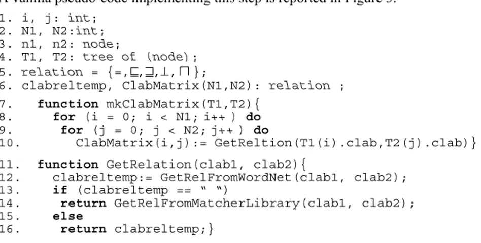
A vanilla pseudo-code implementing this step is reported in Figure 3.
1. i, j: int; 2. N1, N2:int; 3. n1, n2: node;
4. T1, T2: tree of (node); 5. relation = {=, , ,⊥, };
6. clabreltemp, ClabMatrix(N1,N2): relation ; 7. function mkClabMatrix(T1,T2){
8. for (i = 0; i < N1;i++) do 9. for (j = 0; j < N2;j++) do
10. ClabMatrix(i,j):= GetReltion(T1(i).clab,T2(j).clab)} 11. function GetRelation(clab1, clab2){
12. clabreltemp:= GetRelFromWordNet(clab1, clab2); 13. if (clabreltemp == “ “)
14. return GetRelFromMatcherLibrary(clab1, clab2); 15. else
16. return clabreltemp;}
Fig. 3. Computing the CL matrix
T1 and T2 are trees preprocessed by the code in Figure 2. n1 and n2 are nodes of
T1 and T2 respectively, while N1 and N2 are the number of concepts of labels occur-ring in T1 and T2, respectively. ClabMatrix is the bidimensional array memoriz-ing the CL matrix. GetRelation tries WordNet first and then, in case WordNet returns no relation (it returns a blank), it tries the library of weak semantics element
level matchers. In case also this attempt fails, no relation (a blank character) is re-turned.
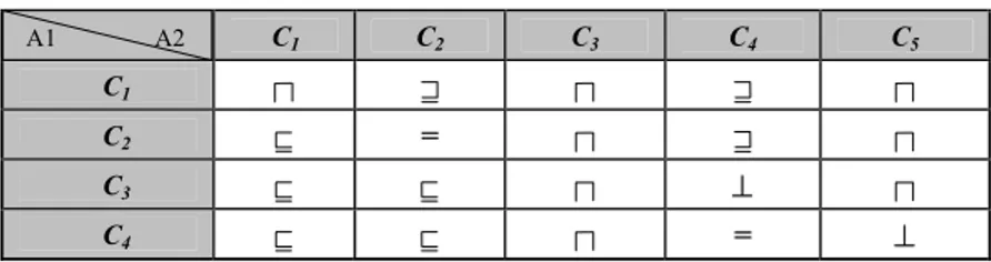
If we apply the code in Figure 3 to the example in Figure 1, we obtain the results in Table 1. In this case, given the input, only WordNet returns useful results.
Table 1: The computed CL matrix of the example in Figure 1
Notice that we have one row for each label in A2 and one column for each label in A1. Each intersection between a row and a column contains a semantic relation. An empty square means that no relations have been found.
3.3 The computation of the CN matrix
The second step at run time (step 4 above) computes the relations between concepts at nodes. This problem cannot be solved simply by asking an oracle containing static knowledge. The situation is far more complex, being as follows:
1. We have a lot of background knowledge computed in the CL matrix, codified as a set of semantic relations between concepts of labels occurring in the two graphs. This knowledge is the background theory/axioms which provide the context (as defined in [9]) within which we reason.
2. Concepts of labels and concepts of nodes are codified as complex propositional formulas. In particular concepts of nodes are intersections of concepts of labels. 3. We need to find a semantic relation (e.g., equivalence, more general, mismatch)
between the concepts of any two nodes in the two graphs.
As discussed in [6], the key idea behind our approach is to translate all the seman-tic relations into propositional connectives in the obvious way (namely: equivalence into equivalence, more general and less general into implication, mismatch into nega-tion of the conjuncnega-tion) and then to prove that the following formula:
Context → rel(Ci , Cj )
is valid; where Ci is the concept of node i in graph 1, Cj is the concept of node j in graph 2, rel is the semantic relation (suitably translated into a propositional connec-tive) that we want to prove holding between Ci and, Cj, and Context is the conjunc-tion of all the relaconjunc-tions (suitably translated) between concepts of labels menconjunc-tioned in
Ci and, Cj. The key idea is therefore that the problem of matching has been translated into a validity problem where the holding of a semantic relation between the concepts of two nodes is tested assuming, as background theory (context), all we have been able to infer about the relations holding among the concepts of the labels of the two graphs. Figure 4 reports the pseudo code describing step 4.
CEurope CPictures CWine CCheese CItaly CAustria
CImages =
CEurope =
CAustria ⊥ =
CItaly = ⊥
1. i, j, N1, N2: int; 2. context, goal: wff; 3. n1, n2: node; 4. T1, T2: tree of (node); 5. relation = {=, , ,⊥, }; 6. ClabMatrix(N1,N2),CnodMatrix(N1,N2),relation:relation 7. function mkCnodMatrix(T1,T2,ClabMatrix){ 8. for (i = 0; i < N1;i++) do 9. for (j = 0; j < N2;j++) do 10. CnodMatrix(i,j):=NodeMatch(T1(i),T2(j),ClabMatrix)} 11. function NodeMatch(n1,n2,ClabMatrix){
12. context:=mkcontext(n1,n2, ClabMatrix, context); 13. foreach (relation in < =, , ,⊥ >) do{
14. goal:= w2r(mkwff(relation, GetCnod(n1), GetCnod(n2)); 15. if VALID(mkwff(→, context, goal))
16. return relation;} 17. return ;}
Fig.4. Computing the CN matrix
CnodMatrix is the bidimensional array memorizing the CN matrix. mkcontext at line 12 builds the context against which the relation is tested. foreach at line 13 tests semantic relations with decreasing binding power. w2r at line 14 translates a relation between two formulas containing only set theoretic connectives into a pro-positional formula. VALID at line 15 is tested by taking the negation of the formula and by testing unsatisfiability by running a SAT decider, namely a decider for pro-positional satisfiability (a formula is valid if and only if its negation is unsatisfiable). In case foreach fails on all the semantic relations in his argument, NodeMatch returns intersection. That this must be the case can be easily proved by reasoning by cases. In fact, given two sets one of the following relations =, , , ⊥ , , must be the case.
The semantic relations computed between all the pairs of CNs for the hierarchies shown in Figure 1 are summarized in Table 2.
Table 2: The computed CN matrix of the example in Figure 1
Each intersection between a row and a column reports the strongest semantic rela-tion that the code of Figure 4 has been able to infer. For example, the concept at node
Images (C1) in A1, is more general then the concept at node Pictures (C2) in A2. Notice that this table, contrarily to Table 1, is complete in the sense that we have a semantic relation between any pair of concepts of nodes. However, the situation is not as nice as it looks as, in most matching applications, intersection gives us no useful information (it is not easy to know which documents should be discarded or kept). [6] suggests that, when we have intersection, we iterate and refine the matching results; however, so far, we have not been able to pursue this line of research.
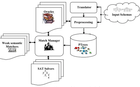
4
A platform implementing semantic matching
Matching is a very hard task. Semantic matching does not have some of the problems that syntactic matchers have. Its major advantage is that the algorithm we have pro-posed is correct and complete in the sense that it always computes the strongest se-mantic relation between concepts of nodes (contrarily to what happens with syntactic matchers, see also the discussion of the testing results in the next section). This is, in fact, an obvious consequence of the fact that we have translated the problem of com-puting concepts of nodes (step 4) into a validity problem for the propositional calcu-lus. However still a lot of problems exist which make it unlikely that we will ever be able to build the “ultimate good-for-all” semantic matcher. Thus, in practice, in se-mantic matching we have not eliminated the problem of incorrectness and incom-pleteness. We have only limited it to the translation of labels into concepts of labels (step 1) and to the computation of the semantic relations existing between pairs of concepts of labels (step 3). Steps 2 and 4, instead guarantee correctness and com-pleteness. However, while, if step 2 is uncontroversial, step 4 still presents problems. These problems are due to the fact that, we have codified the semantic matching problem into a CO-NP problem (as it is the validity problem for the propositional calculus). Solving this class of problems requires, in the worst case, exponential time. Furthermore there is no SAT solver which always performs better than the others and at the moment we have no characterization of our matching problems which allows us to choose the “best” solver and heuristics (even if we have some preliminary evi-dence that most of our examples are in the “easy” part of the “easy-hard-easy” SAT phase transition). A2 A2 C1 C2 C3 C4 C5 C1 C2 = C3 ⊥ C4 = ⊥ A1 A2
Fig. 5. Architecture of the S-match platform
Our approach is therefore that of developing a platform for semantic matching, namely a highly modular system where single components can be plugged, un-plugged or suitably customized. The logical architecture of the system we have de-veloped, called S-Match, is depicted in Figure 5. Let us discuss it from a data flow perspective. The module taking input schemas does the preprocessing. It takes in input trees codified into a standard internal XML format. This internal format can be loaded from a file manually edited or can be produced from a input format dependent
translator. This module implements the preprocessing phase and produces, as output,
enriched trees which contain concepts of labels and concepts of nodes. These en-riched trees are stored in an internal database (the database labeled PTrees in figure 5) where they can be browsed, edited and manipulated. The preprocessing module has access to the set of oracles which provide the necessary a priori lexical and do-main knowledge. In the current version WordNet is the only oracle we have. The
Matching Manager coordinates the execution of steps 3 and 4 using the oracles
li-brary (used here as element level strong semantics matchers), the lili-brary of element level weak semantic matchers, and the library of SAT solvers (among the others, the SAT decider that we are currently testing is JSAT [11]).
S-Match is implemented in Java 1.4 and the total amount of code (without optimi-zations!) is around 60K.
5
A comparative evaluation
We have done some preliminary comparison between S-Match and three state of the art matching systems, namely Cupid [12], COMA [4], and SF [15] as implemented within the Rondo system [14]. All the systems under consideration are fairly compa-rable because they are all only schema-based, and they all utilize linguistic and graph matching techniques. They differ in the specific matching techniques they use and in how they combine them.
Weak semantic Matchers SAT Solvers Match Manager Preprocessing PTrees Oracles Translator Input Schemas
In our evaluation we have used three examples: the simple catalog matching prob-lem, presented in the paper and two small examples from the academy and business domains. The business example describes two company profiles: a standard one (mini) and Yahoo Finance (mini). The academy example describes courses taught at Cornell University (mini) and at the University of Washington (mini).1 Table 3
pro-vides some indicators of the complexity of the test schemas.
Table 3: Some indicators of the complexity of the test schemas
Images/Europe Yahoo(mini)/Standard (mini) Cornell(mini)/ Washington (mini)
#nodes 4/5 10/16 34/39
max depth 2/2 2/2 3/3
#leaf nodes 2/2 7/13 28/31
As match quality measures we have used the following indicators: precision,
re-call, overall, F-measure (from [3]) and time (from [19]). precision varies in the [0,1]
range; the higher the value, the smaller is the set of wrong mappings (false positives) which have been computed. precision is a correctness measure. recall varies in the [0,1] range; the higher the value, the smaller is the set of correct mappings (true positives) which have not found. recall is a completeness measure. F-measure varies in the [0,1] range. The version computed here is the harmonic mean of precision and recall. It is global measure of the matching quality, growing with it. overall is an estimate of the post match efforts needed for adding false negatives and removing false positives. overall varies in the [-1, 1] range; the higher it is, the less post-match efforts are needed. Time estimates how fast matchers are in when working fully automatically. Time is very important for us, since it shows the ability of matching systems to scale up to the dimensions of the Semantic Web, providing meaningful answers in real time.
For what concerns the testing methodology, to provide a ground for evaluating the quality of match results, all the pairs of schemas have been manually matched to produce expert mappings. The results produced by matchers have been compared with expert mappings. In our experiments each test has two degrees of freedom:
di-rectionality and use of oracles. By directionality we mean here the direction in which mappings have been computed: from the first graph to the second one (forward direc-tion), or vice versa (backward direction). For lack of space we report results obtained only with direction forward, and use of oracles allowed.
All the tests have been performed on a P4-1700, with 256 MB of RAM, with the Windows XP operating system, and with no applications running but a single matcher. The evaluation results are shown in Figure 6. From the point of view of the quality of the matching results S-Match clearly outperforms the other systems. As a consequence of the fact that the computation of concept of nodes is correct and com-plete, given the same amount of information at the element level, S-Match will always perform the best and the other matchers can only approximate its results.
1 Source files and description of the schemas tested can be found at our project web-site,
Fig.6. Experimental results
As a matter of fact, the only case where S-Match does not compute precision and recall at their maximum value is due to a mistake in computing the relation between two pairs of concepts of labels. From the point of view of time, S-Match is the lowest, this due to the fact that the computation of mappings in S-Match is translated into a validity problem. However these results do not look so bad as the ratio is always relatively small and, as stated above, the current version of our system has no optimizations.
6 Conclusion
We have presented an algorithm implementing semantic matching and its preliminary implementation within a semantic matching platform, S-Match. We have tested our current implementation against three state of the art systems and the results look very promising, with a point of attention on computation times.
This is only a first step and many issues still need to be dealt with. Some examples are: extend the current algorithm to dealing with attributes (this is of fundamental importance in order to move to the database domain), optimize the algorithm and its implementation, implement iterative semantic matching (as first defined in [6]), do a thorough testing of the system, which in turn will require the definition of a testing methodology, and so on.
Acknowledgments
Thanks to Luciano Serafini, Paolo Bouquet, Bernardo Magnini and Stefano Zanobini for many discussions on CTXmatch. We also thank to Phil Bernstein, Hong Hai Do and Erhard Rahm, Sergey Melnik for providing us with the Cupid, COMA and Rondo prototypes.
Cornell (mini) - Washington (mini)
0.0 0.2 0.4 0.6 0.8 1.0
Rondo Cupid COMA S-match
0.0 2.0 4.0 6.0 8.0 10.0 12.0 14.0 sec
Precision Recall Overall F-measure Time
Simple Cataogs -0.4 -0.2 0.0 0.2 0.4 0.6 0.8 1.0
Rondo Cupid COMA S-match
0.0 0.2 0.4 0.6 0.8 1.0 1.2 1.4 1.6 1.8 2.0 sec
Precision Recall Overall F-measure Time
Average Results 0.0 0.2 0.4 0.6 0.8 1.0
Rondo Cupid COMA S-match
0.0 2.0 4.0 6.0 8.0 10.0 12.0sec
Precision Recall Overall F-measure Time
Yahoo Finance (mini) - Standard (mini)
0.0 0.1 0.2 0.3 0.4 0.5 0.6 0.7 0.8 0.9 1.0
Rondo Cupid COMA S-match
0.0 2.0 4.0 6.0 8.0 10.0 12.0 14.0 16.0 18.0 20.0 sec
References
1. Bergamaschi S., Castano S., Vincini M.: Semantic integration of semistructured and struc-tured data sources. SIGMOD Record, 28(1) (1999) 54-59.
2. Bouquet P., Serafini L., Zanobini S.: Semantic coordination: A new approach and an appli-cation. Proceedings of ISWC, (2003) 130-145.
3. Do H.H., Melnik S., Rahm E.: Comparison of schema matching evaluations. Proceedings of workshop on Web and Databases, (2002).
4. Do H.H., Rahm E.: COMA – A system for flexible combination of schema matching ap-proaches. Proceedings of VLDB, (2002) 610-621.
5. Doan A., Madhavan J., Domingos P., Halevy A.: Learning to map between ontologies on the semantic web. Proceedings of WWW, (2002) 662-673.
6. Giunchiglia F., Shvaiko P.: Semantic matching. In The Knowledge Engineering Review journal 18(3) (2003) 265-280. Short versions: Proceedings of Ontologies and Distributed Systems workshop at IJCAI and Semantic Integration workshop at ISWC, (2003).
7. Giunchiglia F., Zaihrayeu I.: Implementing database coordination in P2P networks. Pro-ceedings of the workshop on Semantics in Peer-to-Peer and Grid Computing at WWW (2004).
8. Giunchiglia F., Zaihrayeu I.: Making peer databases interact - a vision for an architecture supporting data coordination. Proceedings of international workshop on Cooperative In-formation Agents, (2002) 18-35.
9. Giunchiglia F.: Contextual reasoning. Epistemologia, special issue on "I Linguaggi e le
Macchine", vol. XVI, (1993) 345-364.
10. Kang J., Naughton J.F.: On schema matching with opaque column names and data values. Proceedings of SIGMOD, (2003) 205-216.
11. Le Berre D. JSAT: The java satisfiability library. http://cafe.newcastle.edu.au/daniel/JSAT/. (2001).
12. Madhavan J., Bernstein P., Rahm E.: Generic schema matching with Cupid. Proceedings of VLDB, (2001) 49-58.
13. Magnini B., Serafini L., Speranza M.: Making explicit the semantics hidden in schema models. Proceedings of workshop on Human Language Technology for the Semantic Web and Web Services at ISWC (2003).
14. Melnik S., Rahm E., Bernstein P.: Rondo: A programming platform for generic model management. Proceedings of SIGMOD, (2003) 193-204.
15. Melnik, S.,Garcia-Molina H., Rahm E.: Similarity flooding: A versatile graph matching algorithm. Proceedings of ICDE, (2002) 117-128.
16. Miller, A.G.: Wordnet: A lexical database for English. Communications of the ACM, 38(11) (1995) 39-41.
17. Rahm E., Bernstein P.: A survey of approaches to automatic schema matching. VLDB journal, 10(4) (2001) 334-350.
18. Xu L., Embley D.W.: Using domain ontologies to discover direct and indirect matches for schema elements. Proceedings of Semantic Integration workshop at ISWC, (2003). 19. Yatskevich M.: Preliminary evaluation of schema matching systems. Technical Report,