Sociality in Complex Networks

(1)

Sociality in Complex Networks

Universit`

a degli Studi di Catania

Dipartimento di Ingegneria Elettrica, Elettronica e dei Sistemi

(2)

Abstract

The study of network theory is nothing new, as we may find the first example of a proof of network theory back in the 18th century. However, in recent times, many researchers are using their time to investigate networks, giving new life to an old topic. As we are living in the era of information, networks are everywhere, and their complexity is constantly rising. The field of complex networks attempts to address this complexity with innovative solutions. Complex networks all share a series of common topological features, which revolve around the relationship between nodes, where relationship is intended in the most abstract possible way. Nonetheless, it is important to study these relationships because they can be exploited in several scenarios, like web page searching, recommender systems, e-commerce and so on. This thesis presents studies of sociality in complex networks, ranging from the microscale, which focuses the attention on the point of view of single nodes, to the mesoscale, instead shifts the interest in node groups.

(3)

Declaration

I declare herewith, that this dissertation is my own original work. Furthermore, I confirm that:

• this work has been composed by me without assistance; • I have clearly referenced all sources used in the work;

• all data and findings in the work have not been falsified or embellished; • this work has not been published.

(4)

Chapter 1 Introduction

In network theory, a network (or graph) is a model that aims at abstracting the symmetric or asymmetric connections among entities. The concept of a network is definitely not new in the field of mathematics, dating back to 1735, when Euler provided what it has been called the first proof of network theory: the solution to the K¨onigsberg bridges problem. Since then a lot has changed, the real world has become increasingly more complex, and in the age of computer science, networks are everywhere. Networks have increased in complexity too: things like web-based social networks or the world wide web are monstrous entities that are made of billions of nodes. But it’s not just the amount of nodes that makes the study of these networks more difficult, as the most interesting aspect of these networks are the way the links are distributed. At a first glance, no clear pattern appears, and nodes seem to be randomly interconnected, while in reality their connections are neither regular not random, but somewhere in-between. Basically, there is a sort of regularity in the randomness, as these networks share the same interconnection patterns. A lot of effort has been put into the research of these patterns, which over time has created a specific research field, which is the field of complex networks. To

(7)

summarize, a network is complex when it displays non-trivial topological features. Some of the features that are shared among complex networks are:

• heavy tail in the degree distribution; • high clustering coefficient;

• assortativity or disassortativity among vertices; • hierarchical structure;

• community structure.

Firstly, the degree distribution of complex networks can be heavy-tailed: which means there are many nodes that have a low degree, and few nodes that have an high degree. Nodes also tend to cluster themselves together, resulting in an unusually high clustering coefficient. The way nodes are clustered together depend on the type of network: in social networks nodes tend to form links with nodes that are similar, showing assortativity, while in biological networks entities seek diversity in their connections, showing a certain degree of disassortativity. Moreover, in networks with a significant amount of clusters, cluster themselves may sometimes be grouped in ”clusters of clusters”, effectively forming a hierarchical structure. But the last feature in particular has attracted the interest of many researchers, which is a property of the node clusters themselves, the community structure. The definition of community is controversial, but the general consensus is that a set of nodes may be grouped in a community if they are densely interconnected among each other. Community structure inside complex networks suggests that there is a somewhat natural division among the network nodes that emerges from the network itself. Finding these communties has become an hot topic in the field of complex networks, as

(8)

the increased complexity presents new challenges and obstacles that need to be addressed (literature review on the matter in Chapter 2).

Note that the list provided is not complete nor mandatory, there are indeed complex networks that, for example, are not heavy-tailed in the degree distribution. Hoewver, most complex networks share at least some of those properties compared to random networks, and they represent a hint that the network under exam is indeed complex. Of all the properties mentioned above, my work has mostly focused on assortativity, community structure and clustering. I found myself studying how nodes arrange themselves in groups, and asking myself why. In a certain sense, my approach was analogous to a sociologist’s. After all, some complex networks are indeed models of social networks, but the social behavior also extends to other types of networks as well. If we take the concept of homophily, for example, and extend it to other types of entities in complex networks, we find that it maps quite gracefully to the idea of assortativeness.

There are plenty of other social features and properties in the realm of complex networks: as already mentioned nodes tend to arrange themselves in groups. These groups are hardly static in nature, and they change over time. The dymamics that rule these changes are, again, social-based. My work in the past three years was focused on different things, but the common theme is that I tried to investigate social behaviour in complex networks. There are many real world applications of these studies. In web page ranking, for example, it is important to anaylize how web pages are linked to each other to assess the relevance of a certain web page. Information such as the number of outlinks, the number of inlinks, which pages are pointed and which pages point to our page, is very useful to determine its importance. In the e-commerce scenario, we want to have a successful transaction, so we are looking for trustworthy nodes to interact with. Trustworthiness is assessed by

(9)

evaluating what other nodes ”think” of the node we wish to contact. It is then essential to abstract the level of trustworthiness that a node places on his neighbours by giving them a score, or trust value. This score is an extremely condensed and simplified measure of how we trust that neighbour, and usually depends on the past history between the two nodes. If we had a history of successful interactions, the resulting score will be higher, and vice-versa. Recommender systems also make use of social interactions to predict which product to suggest. They see which products are commonly bought by similar users and suggest them to the same class of users. This of course requires clustering users that share the same interests in the same group.

My work during the past three years consisted in studying sociality in complex network. The focus was mainly on three facets of sociality: trust, communities, and popularity, intended as the importance of the node in the network. I have studied how to model trust out of metadata information [1, 2], how to raise the importance of a node in the network [3], how to assess the importance of a node [4], and how to evaluate the quality of a specific partition in communities [5, 6].

This thesis is structured as follows. Chapter 2 provide a succint review of the literature about topic inherent to this thesis. Chapter 3 describes research done in the microscale, where the emphasis is on nodes. On the contrary, Chapter 4 gives a broader point of view, focusing on the research done for groups and communities. At last, Chapter 5 reviews the content of this thesis.

(10)

Chapter 2 Related Works

This section will provide a succint summary about the state of the art of the three most important topics discussed in this thesis: trust networks, ranking algorithms and community detection.

2.1 Trust networks

Over the last decades, he term trust has been characterized with different meanings [7, 8, 9, 10, 11], depending on which context is considered (e.g. sociology, psychology and so on). Although there is no definitive agreement on these various definitions of trust, most researchers agree from the early beginning [12] that it is fundamental whenever an individual takes a risk and there is uncertainty about the outcome [13].

Given that the definition of trust itself is not universal, establishing whenever a certain node trusts another is not an easy task, and requires data aggregation strategies. In [14], the authors provide an overview of the most recent achievements and open challenges about Big Data mining. It is also important to take into account the trustworthiness of the collected data to obtain trust information about the users [15, 16].

(11)

Trust modeling goes according to the context: links model trust in trust networks, hy-perlinks in website ranking, or buyer-seller relationships in the e-commerce context. In ICT context [17] trust is a leading tool for computers and software agents to discriminate themselves among good and bad ones, its role in broader scenarios is steadily increasing, in particular when humans communicate with others in virtual environments [18], with on-line services [19, 20], with intelligent pervasive environments [21] and so on [22, 23, 24, 25, 26, 27]. In all these situations indeed people generally have to provide some of their personal information in order to positively fulfill the interaction, and they rely on

trust as a key factor to establish whether the counterpart is worth to connect to.

Trust network frameworks [28, 10, 29, 30] model the trust network as a graph where nodes are agents (persons) and trusting relationships are directed arcs weighted using a measure of the direct trust value according to a given metric. As pointed out by Artz and Gil [31] trust can be intended as a measure of how good the future behavior of a given agent will be based on his past actions, in other words the reputation can be considered as an effective approach for trust assessment. Many trust assessment algorithms, such as EigenTrust [32], Powertrust [33] and GossipTrust [34], use the feedback mechanism to evaluate the trustworthiness of an agent.

Despite the importance of neighbours in the definition of trust, existing literature mainly focuses on the assessment of global trust, i.e. the unique value for a node that aims at mediating all direct values that express different judgements the node received from others. A work that strengthened the role of local trust is TrustWebRank [35], where different trust values can be assigned by distinct nodes to the same one. The need for local trust is supported also by other researchers, e.g. [36] claims that local values are needed when a shared opinion cannot be achieved (controversial nodes). Finally, the local

(12)

approach is more precise and tailored to the point of view of each user and also more attack-resistant to malicious peers [37].

2.2 Ranking algorithms

Ranking algorithms are algorithms that process node metadata and topology information, and produce an ordered list of nodes. The order of the nodes has different meanings according to the ranking algorithm employed but, in general, higher positions are assigned to nodes which are more relevant to the specific algorithm. Relevance depends on the scenario being considered: in web searching relevance is measured against a given search query [38, 39, 40], in E-learning resources must be relevant to a given topic [41, 42, 43], in a recommendation network the most reliable nodes are the most relevant [44, 45, 46, 47, 48, 49], which is also true for e-commerce scenarios [50, 51].

One of the most important ranking algorithms is PageRank[52, 53]. PageRank is es-sentially an application of the random walker model on a Markov chain: the nodes of the Markov chain are the web pages, and the arcs are the links that connect one page to another. The walker represents a generic web surfer which moves from page to page with a certain probability, according to the network structure, and occasionally ”gets bored” and jumps to a random node in the network. The steady-state probability vector of the random walker process holds the PageRank values for each node, which can be used to determine the global ranking. Although Pagerank was proposed a long time ago, it still lives as the backbone of many technologies, not limited to the web domain. For example, in [54], personalized PageRank is cited as a possible algorithm to be used in Twitter’s ”Who To Follow” architecture. In [55], the author shows how the mathematics behind PageRank have been used in a plethora of applications which are not limited to

(13)

ranking pages on the web. In [56], another PageRank extension appears as a tentative replacement of the h-index for publications.

PageRank has to face a plethora of competitors in several application domains. In the web domain we have HITS [57], which is not based on the random walker model and is able to provide both an ”authority” ranking, which rewards nodes that have many backlinks, and a ”hub” ranking, which rewards nodes that have many forward links. SALSA [58] computes a random walk on the network graph, but integrates the search query into the algorithm, which is something PageRank does not do. In the trust networks domain we have PeerTrust [33], which computes the global trust by aggregating several factors, and PowerTrust [59] which uses the concept of ”power nodes”, which are dynamically selected, high reliability nodes, that serve as moderators for the global reputation update process. The PowerTrust article also describes how the algorithm compares to EigenTrust with a set of simulations that analyse its performance. Several articles feature side-by-side comparisons among PageRank (and its extensions) and other metrics [60, 61, 62]. In particular, [63] focuses on comparing HITS, PageRank and SALSA, and its authors prove that PageRank is the only metric that guarantees algorithmic stability with every graph topology.

2.3 Community detection

Even the community detection problem is not new in the domain of graph theory. The analysis of communities provides a deeper knowledge of the network’s structure and the correlation between nodes, which allows the study of the information embedded into net-works. Networks concerning healthcare, infection spread, human interactions, economics, transportation, trust and reputation are perfect examples where detecting communities

(14)

can help to understand the network’s structure.

The definition of a community itself is, again, controversial. Intuitively, it can be defined as a set of entities that are close to others. This notion is quite similar to the concept of closeness, which is based on a similarity measure and is usually defined over a set of entities. One of the most acknowledged definitions of community appears in [64]. This definition has given birth to several algorithms for community detection [65] [66] which, for the most part, rely on the optimization of a validation function measuring the quality of the community structure. One of the most commonly used functions is the modularity function provided by Newman [64, 67]. Despite some limitations [68, 69], the modularity function has been successfully used as a quality measure to evaluate a given network partition and as a cost function to be optimized to uncover communities [70, 71, 65]. Other than modularity based methods, in literature there exists a lot of alternative ap-proaches to solve the problem of community discovering [72, 73]. For example, in Ref. [74] an information-theoretic based method is presented. This method is based on the formu-lation of a new quality function called map equation[75], which allows to find the optimal description of the network by compressing its information flow. The algorithm is the core of Infomap (http://www.mapequation.org/), the search method for minimizing the map equation over possible network partitions.

Community detection has been successfully used to analyze the structure of single-layer networks and for modeling several kinds of interactions, such as social relationships, genetic interactions among biological molecules or trade among countries [76, 77, 78, 79, 80, 81, 82], just to mention a few (a detailed introduction to communities in networks can be found in [72, 73]).

(15)

Chapter 3 Microscale

There are two basic units that form a network graph, nodes and edges (or arcs, if the graph is directed). However, edges are merely used to model connections between nodes and, to a certain extent, they can be seen as node metadata. Given this thesis’ focus on sociality, it is only natural to start the discussion from the point of view of nodes, the

microscale: which neighbours should a node have? how does a node model its relationship

with them? how do its neighbours impact its popularity in the network? This section will present the answer to these questions through theory, methodologies and simulations.

3.1 Local Weight Assignment

In a social network, the problem of assigning local weights consists in finding what weights should be given to a node’s neighbours based on a certain set of metadata. The arc weights are an abstraction of the relationship between the two nodes, and should be based on social metadata in order to accurately model the quality of such relationship. As mentioned, it’s difficult to talk about relationships without mentioning trust, and indeed many social networks are grounded on trust relationships. In a certain way, we

(16)

could say that social networks are a general case of trust networks.

A trust network is a network where the edges specifically model the level of trust that the two connected nodes share. In the past years, trust networks have grown in popularity as a fundamental precautionary component that helps users in managing virtual interactions with (possibly total) strangers, either real people or virtual entities, in several contexts such as e-commerce, social networks, distributed on-line services and many others [83, 84, 19].

Generally, in trust models and frameworks developed in the past years [28, 10, 29, 30], the trust network is represented as a graph where nodes are agents and trusting relationships (arcs) are weighted against a measure of the direct trust value according to a given metric. Sometimes trust networks may even be signed, because a negative weight may be associated to the lack of trust, or distrust, even though it’s much harder to handle signed graphs due to algorithmic issues.

While most of the existing literature focuses on the assessment of global trust, i.e. the unique value for a node that aims at mediating all local (direct) values that express different judgements the node received from others, there is less emphasis on how direct trust should be evaluated for each node i.

In many scenarios, the successful, positive interactions between two nodes are taken into account in order to produce a trust value, which will be modeled by the arc weight con-necting the two nodes. The well known proposals EigentTrust [32] and GossipTrust [34] compute direct trust following this principle. However, in order to provide a weight as-signment model based on real world social criteria, there are two additional factors that need to be taken into account, the mistrust as a measure of a lack of trust, and the

(17)

Symbol Description

N Number of neighbors

R Total number of interactions among all neighbors

ri Interactions with neighbor i

r_i+ Positive interactions experienced with neighbor i r_i− Negative interactions experienced with neighbor i

Table 3.1: Notation in use

balance positive and negative feedbacks when selecting a node, and popularity measures to what extent a certain trust or mistrust rating is relevant. This way, a node which has more positive feedbacks than negative feedbacks it is considered overall trustworthy, and a node with more feedback scores is considered more trustworthy than a node with less feedback scores, if the overall trust rating is the same.

In the paper[2], the authors propose a direct trust assessment model, and prove, through a series of simulations, that it exhibits greater stability compared to EigentTrust and GossipTrust, i.e. if a node changes its behavior, trust and mistrust ratings are not signif-icantly affected, unless this behavior repeatedly occurs, as the proposed model also takes into account the node’s history (if a node has received hundreds of positive feedbacks, it takes more than a few incoming negative feedbacks for it to be considered untrustworthy).

3.1.1 Local Trust assessment

Notation and existing approaches

There are several possible intuitive approaches to assign weights to the arcs of a trust network. In this work, some of them will be analyzed for possible shortcomings. Before this, let’s introduce a few definitions of the quantities involved for ease of notation, which are reported in Table 3.1. Alongside these definitions, let’s introduce three new quantities:

(18)

pi = ri R, ti = r_i+ ri , mi = r−_i ri = 1 − ti (3.1)

pi is the popularity of neighbor i seen from the perspective of a certain node n, ti the trust

that node n places in neighbor i and mi the distrust that node n places in neighbor i.

There are several works about the coexistence of trust and distrust in literature: in [85] propagation of trust and distrust is analyzed, whereas in [86] the authors manage to predict with acceptable accuracy whether a node is going to trust or distrust another node which is not connected to; finally, in [87], an extension of PageRank which works on signed graphs named PageTrust is introduced.

The approach described in [2] attempts to take into account both trust and distrust, incorporating them in a single weight assignment criterion. One of the most intuitive ways to model the node’s attitude in a trust network is to give a Positive Feedback. It can be obtained by normalizing the positive interactions:

w+_i = r + i ∑N k=1r + k (3.2)

However, this solution does not make use of negative interactions. A node which ex-periences a negative interaction with a neighbor, should alter its attitude towards that neighbor accordingly. Intuitively, an agent wants to avoid more those nodes it had nega-tive interactions with, and equation (3.2) does not take this aspect into account.

Another intuitive way to model the node attitude is to give Net Feedback, that tries to incorporate negative interactions into the weight equation, as done by EigenTrust. Naming f+ i = max(0, r + i − r − i ), we have: w+_i = f + i ∑N k=1f + k (3.3)

(19)

While this approach does include negative interactions in the arc weight, it has one important shortcoming: it reacts very poorly to feedback changes. Let us suppose we have a neighbour with 100 positive feedback ratings and 99 negative feedback ratings. With this equation, its f+

i would be 1. If our node completes another interaction with

this neighbour positively, its f+

i will change to 2. This feedback gain essentially doubles

the previous value, and this doesn’t model well the mixed behavior of the node.

Social-based weight assignment

Taking note of issues described so far, the idea is to provide a weight equation that models the attitude according to these features:

• Neighbors with more interactions should be preferred. If two neighbors have the same ratio r_i+

ri, the one with the largest ri should be more likely to be contacted.

• The higher negative/total interactions ratio a neighbor has, the more it should be avoided.

• The higher positive/total interactions ratio a neighbor has, the more it should be contacted.

• It should take into account previous interactions.

A node should weight both popularity and trust when making a decision about the trustworthiness of a certain node. A popular, trustworthy node is more likely to yield a successful interaction than a less popular node with the same level of trustworthiness. At the same time, we want to take into account the distrust of other nodes. This is because the more untrustworthy a node is, the more we want to avoid having interactions with it. This criterion to assign weights in a trust-based network, named social weight

(20)

assignment, sports two different components: the trust towards node i and the average

distrust of all neighbors except i; both components are linear dependent on the neighbor popularity.

Definition and meanings

The social weight assignment criteria assigns the following weight to node neighbors:

w_i+= tipi+ N ∑ k=1,k̸=i mkpk N −1 (3.4)

where N is the number of neighbour nodes of node n. It is easy to prove that∑N

i=1w + i = 1: N ∑ i=1 w_i+= w₁++ w₂++ . . . + w_N+ = t1p1+ N ∑ i=1,i̸=1 mipi N −1 + t2p2+ N ∑ i=1,i̸=2 mipi N −1+ . . . + + tNpN + N ∑ i=1,i̸=N mipi N −1 = N ∑ i=1 tipi+ N ∑ j=1 N ∑ i=1,i̸=j mipi N −1 (3.5)

Note that in the double sum each mipi is repeated N − 1 times so we may reduce the

notation as: N ∑ i=1 tipi + N ∑ i=1 mipi = N ∑ i=1 (ti + mi)pi = N ∑ i=1 ( r+_i ri + r−_i ri ) ri R = N ∑ i=1 ri R = 1 (3.6)

This result allows to apply the social weight assignment in conjunction with metrics that require that the sum of the node outlink weights is 1, as all EigenTrust-based proposals. It is also possible to define a dual criterion with the same entities defined in (3.1), where

ti and mi are swapped:

w−_i = mipi+ N ∑ k=1,k̸=i tkpk N −1 (3.7)

(21)

These two criteria generate two different networks, a trust network for the social weight assignment, and a distrust network for its dual. These two networks are not complemen-tary, in-fact, while they share the same topology, the arc weights are different: weights of the trust network cannot be derived directly from the weights of the distrust network, and vice-versa.

This implies that the node with highest weight in the trust network (the ”best node”) is not necessarily the node with the least weight in the distrust network. Another conse-quence of the way the weights are assigned is the fact that the most reliable node isn’t necessarily the best node, as its trust weight is multiplied by pi: the popularity of the

node (which essentially means the portion of the node interactions shared with neighbour

i) impacts greatly the final weight. This is by design, as the more interactions the node

has with a neighbour, the more reliable the trust (or distrust) weight is: a node with 0.9 trust and 0.1 popularity has a lower weight than a node with 0.8 trust and 0.6 popularity in the trust network. This is in line with the behavior of human beings in a social context. An aspect that is interesting to expand upon a bit is how a neighbor is judged in trust and distrust networks. There are three possible situations:

• Trustworthy node: node has higher trust weight than distrust weight. These nodes are obviously the most reliable, especially if they have high popularity.

• Mixed node: node has similar trust and distrust weight. This can happen when the trust weight is near to the distrust weight.

• Non-trustworthy node: node has higher distrust

weight than trust weight. These nodes should be avoided, regardless of popularity. It is clear that a node should not react in a symmetric fashion to trust and distrust:

(22)

trust is easily shaken, but hard to build up. Future work may define a behavioral pattern for nodes using this weight assignment criteria. In conclusion, the two criteria provide the end-user with different information, which can be used together to make informed decisions about which nodes to trust, and which nodes to avoid.

3.1.2 Modelling the aging of interactions

While the social weight assignment equation (3.4) attempts to model social behavior, it is purely atemporal in meaning, as it doesn’t keep track of the age of the interactions. In the realm of social interactions, older experiences and memories tend to have a reduced degree of impact on our behavior towards a certain person. Indeed, older memories get weaker over time, and their decline in strength has been the object of research for mathematical psychologists up to this day [88]. In particular, they strive to bind the memory detention decline to a mathematical function usually called forgetting curve.

The aging function proposed in this paper loosely takes inspiration after the forgetting curve modeling effort that has been pursued by researchers. This aging function aims at evaluating the contribution of experiences that have a certain age to the arc weight. The aging function candidates a(T ) should manifest three properties:

• a : R≥0 →(0, 1]

• a(0) = 1

• monotonically decreasing

Given that the aging function is time-continuous, the age of a certain interaction that occurred at time t0 can be written as T = t−t0. Finally, if we wanted to know the weight

(23)

T_ij+ (T_ij−) the age of the j-th positive (negative) interaction that occurred with neighbor i we may define the following aging parameters:

A+_i = r_i+ ∑ j=1 a(T_ij+) A−_i = r_i− ∑ j=1 a(T_ij−) Ai = A+i + A − i

that can be used to modify (3.1):

p′_i = _∑_NAi i=1Ai , t′_i = A + i Ai , m′_i = A − i Ai , (3.8)

The values in (3.8) can then be used in (3.4) to compute the weight of the arc towards neighbor i.

Candidates

We propose two candidate families of functions that manifest the aforementioned prop-erties and could model the aging functions: exponential functions e(t) = e−βt _{and power}

functions p(t) = (1 + αt)−β_{, with α, β ∈ R}

>0. They both behave similarilly, except that

the exponential functions decrease much more quickly after a certain ¯t, which depends on the choice of parameters. The candidate aging functions as they are have an infimum of 0, as their limit for t → +∞ is 0. This means that the strength of each interaction fades until it stops to be a significant contribute to the arc weight. This might not be desired in all application scenarios, as older interactions essentially get ignored after a certain amount of time. To prevent this behavior, we changed the candidates in the following way:

(24)

Where γ ∈ R>0. This way we have that both candidates have an infimum greater than

zero, meaning that after a certain amount of time γ the interactions ”stop aging” and keep contributing to the arc weight with a constant value.

Implementation

Regrettably, the implementation of the aging functions is not a trivial task. The main issue comes from the difficulty in finding an appropriate time representation. As said before, the aging functions candidates are time-continuous. This makes them unfeasible candidates as they are, since all software or hardware clocks are time-discrete. The first challenge is then finding a correct quantization step. Intuitively, it should be small enough so that each interaction would lie in a separate time slot. Unfortunately, there’s no easy way to predict the expected time of arrival of each interaction in real-world scenarios. In order to solve the issue it’s better to discard the idea of a timestamp: each node would now evaluate the passage of the time based on the number of interactions. This virtualization of the notion of time based on the number of past interactions means that having an age T would imply being ”T interactions old”. This approach also avoids the issue of time synchronization among nodes, which would require a significant effort. Of course this makes the time completely virtual, so it is not possible to assess the times-tamp of a specific interaction among two peers at network level. This can be troublesome e.g. if we want to analyze the network behaviour at a certain time by reading which interactions happened at that time. Due to the virutalization, it’s only possible ensure that interactions are accounted for in the proper order, there’s no possibility of using a reference time, a sort of wallclock. This is acceptable, however, since social weight assignment criterion operates locally, and is unaware of everything that happens beyond

(25)

the line of sight of each node.

In order to correctly implement aging two challenges need to be overcome, updating the age of all interactions whenever a new interaction occurs, and computing the age parameters Ai, A+i and A

−

i to be used in (3.8). With some bit-level manipulation is fairly

easy to design a storage-efficient solution to both problems. For each neighbor i, we need to allocate four entities:

• A γ-bit binary register b+

i for positive interactions

• A γ-bit binary register b−

i for negative interactions

• A counter c+

i for positive interactions having an age greater than γ

• A counter c−

i for negative interactions having an age greater than γ

A set bit in position k in registers b+

i and b

−

i means that there is an interaction with

neighbor i of age k. This way the age increses along with the bit position, so that the MSB is the oldest interaction that can be stored in the register, which always has age

γ −1. The counters c+_i and c−_i are used to keep count of the interactions which age is

equal or greater to γ. Updating the interaction age is then a matter of using appropriate bit-manipulation operators as described in Algorithm 1. We can see that increasing the age of all interactions is done by applying a bit-shift operator on the whole register (lines 5 and 9). However, this destroys the content of the MSB, so we need to transfer its content to the appropriate counter prior to the operation. This is done in lines 2-3 and 6-8. Note that this needs to be done for each neighbor (line 1), even those who don’t take part in the current interaction, as age is based on the number of interactions that occur among all neighbors. After the age is updated, we simply check whenever the current interaction is successful, and set the LSB, which has an age of 0, of the counter tied to

(26)

the neighbor i (lines 11-15). Algorithm 1 is used to keep track of the virtual time, but it

Algorithm 1 Age update after interaction with neighbor i

1: for j ←1 . . . N do 2: if b+_j & (1 ≪ γ − 1) then 3: c+_j ← c+ j + 1 4: end if 5: b+_j ← b+_j ≪1 6: if b−_j & (1 ≪ γ − 1) then 7: c−_j ← c−_j + 1 8: end if 9: b−_j ← b−_j ≪1 10: end for

11: if interaction is successful then 12: b+_i ← b+

i |1

13: else

14: b−_i ← b−_i |1

15: end if

is also necessary to calculate the three age parameters Ai, A+i and A

−

i . This is described

in Algorithm 2. The value in counters c+

i and c

−

i stands for the number of interactions

that have an age greater than or equal to γ, so it’s possible to initialize A+

i and A

−

i

employing the appropriate counter, like in lines 1-2. Estimating the contribute of fresher interactions require checking each bit of registers b+

i and b

−

i : if a bit in position k is set,

its contribute to the corresponding register is equal to a(k) (lines 3-10).

Algorithm 2 Computation of Ai, A+i and A

− i 1: A+_i ← c+ i · a(γ) 2: A−_i ← c−_i · a(γ) 3: for T ←0 . . . γ − 1 do 4: if b+_i & (1 ≪ T ) then 5: A+_i ← A+ i + a(T ) 6: end if 7: if b−_i & (1 ≪ T ) then 8: A−_i ← A−_i + a(T ) 9: end if 10: end for 11: Ai ← A+i + A − i

(27)

3.1.3 Simulation

In this subsection, we present a set of simulations that compare the behavior of several weight assignment criteria. The results show that the social weight assignment is resilient to changes, and that it is sensitive to nodes which behave in a different way from the others. We also experimented with the two aging function candidates (3.9) to see which function affects more arc weights evaluation.

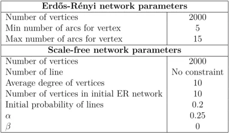
The devised simulation scenarios share a common set of rules, related to the weight as-signment strategy described by equation (3.4). The networks in which weight asas-signment techniques are tested are either scale-free or modeled after Erd˝os-R´enyi graphs. They are generated using the software Pajek [89] using the parameters in Table 3.2.

Erd˝os-R´enyi network parameters

Number of vertices 2000

Min number of arcs for vertex 5

Max number of arcs for vertex 15

Scale-free network parameters

Number of vertices 2000

Number of line No constraint

Average degree of vertices 10

Number of vertices in initial ER network 10

Initial probability of lines 0.2

α 0.25

β 0

Table 3.2: Network parameters

After the networks are generated, their evolution is simulated. We divided the simu-lations in several cycles. For each cycle, each node simulates an interaction with each of its neighbors. This interaction can have a positive, or negative outcome, which is permanently recorded by the node as a positive or negative experience.

The outcome of a transfer is determined at random according to an uniform distribution. The distribution itself depends on the node receiving the interaction, which can be a

(28)

”good” or a ”bad” node. Whether a node is ”good” or ”bad” is determined at the beginning of the simulation, according to these simple rules:

• 95% of the nodes have at most a 20% chance of unsuccessfully replying to a transfer request (”good” nodes).

• 5% of the nodes have at least 80% chance of unsuccessfully replying to a transfer request (”bad” nodes).

• The bad nodes are picked at random following a uniform distribution.

In each simulation, PageRank for a specific node, the ”monitored node” is computed, and changes in its PageRank value cycle after cycle are monitored. Once a node is assigned a certain behavior, it does not change it during the course of the simulation. An exception to this is the monitored node described below. Also, nodes do not have ”favourite” neighbors: each neighbor asking for an interaction is treated equally by the receiving node.

Computing PageRank on the network where the social weight assignment was applied is always possible since the equations guarantee that the outstrength of each node is exactly 1, making the adjacency matrix row-stochastic. The monitored node is always the node which has the highest ”topological PageRank”, that is, the PageRank calculated when all arcs in the network have unitary weight. The simulation graphs always show this PageRank for each cycle. As already mentioned, the monitored node does not follow the behavioral rules described above.

Finally, the aging functions employed in the simulation are the two candidates defined in (3.9). The parameters used in the simulation for the candidates are shown in in Table 3.3.

(29)

α β γ

Exponential N/A 0.065 64

Power 1 1 64

Table 3.3: Aging functions candidates parameters

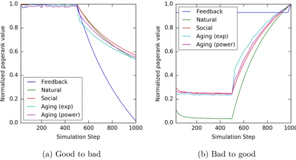
(a) Good to bad (b) Bad to good

Figure 3.1: Comparison among different weight assignment techniques in a network where some nodes behave poorly.

The goal of the simulations is to compare the behavior of the Social Weight Assignment against the other techniques described in subsection 3.1.1, i.e. the Positive Feedback approach, and the Net Feedback approach, and to establish the effect of aging applied to our Social Weight Assignment. In these simulations, the behavior of the different weight assignment techniques for a 2000 nodes scale-free network is displayed. The normalized PageRank value of the monitored node is plotted against the simulation steps, and the results for all weight assignment criteria are shown in Figure 3.1. The normalized value is used to show the relative difference among the techniques, as the absolute PageRank value by itself is meaningless.

The net feedback approach (blue line) drops much faster in simulation 1a compared to the other weight assignment criteria, and behaves quite poorly in simulation 1b. The behavior of Social (red line) and Natural (green line) Feedback approaches is quite similar, but the

(30)

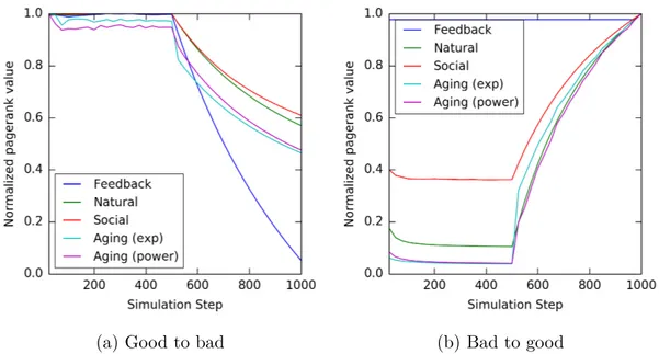
(a) Good to bad (b) Bad to good

Figure 3.2: Comparison among different weight assignment techniques in a network where all nodes behave properly.

Social approach reacts more slowly to changes. Due to this difference of slope, the two curves cross at a certain simulation step.

It is interesting to highlight the trend of the two aging functions (exponential, in teal, and power, in magenta). They highlight the presence of a shock when the node changes behavior, as its PageRank value drops (1a) or raises (1b) immediately. This is due to how the aging model works, as newer experiences can weight several orders of magnitude more than older experiences: this ensures that the model reacts very fast to sudden behavior shifts. While being a consequence of the mathematical model employed, this effect is coherent with the social aspect of the proposed criterion, as it reflects the surprise factor of a person which faces unexpected behavior from a peer they had a certain idea of. After the shock, the two curves’ slopes are comparable to the slope of the non-aging social weight assignment curve. The exponential aging function has a greater effect on the shock phenomenon compared to the power-based aging function.

Simulation 2 has same setup of simulation 1 but the error rate has been set to 0 (that means that all nodes always behave properly). The overall trend of the data analyzed

(31)

in Simulation 2 is similar to the trend of data in simulation 1a and 1b, but the slope of the social approach is steeper. This is because the Social weight assignment tends to highlight neighbors which behavior differs from the average. The two curves about the aging effect show no different behavior compared to simulation 1, so the same things can be said concerning their trend.

In conclusion, the simulations show that the social weight assignment criteria is more stable compared to the presented techniques. Moreover, it successfully reacts to sudden behavior changes (shocks) if we add the aging paramenter to the weight assignment. No other difference in terms of behavior are present between the two curves employing the aging function candidates, besides the already mentioned slope steepness.

3.2 Best Attachment

Ordering nodes by rank is a benchmark used in several contexts, from recommendation-based trust networks to e-commerce, search engines and websites ranking. During the past years it emerged in several scenarios, from trust-based recommendation networks [48, 49] to website relevance score in search engines [39, 40], e-commerce B2C and C2C trans-actions [50, 51]. Within each specific framework, different proposals exist about the meaning of nodes (agents, peer, users) and about the rank assessment algorithm; in all of them, the higher is the rank of a node, the higher is its legitimacy. The rank depends on the set of out-links each node establishes with others [90], and on the set of in-links it receives.

In the mentioned scenarios, the node rank depends on the set of links the node estab-lishes, hence it becomes important to choose appropriately the nodes to connect to. The problem of finding which nodes to connect to in order to achieve the best possible rank

(32)

is known as the best attachment problem. Given that the network is usually modeled as a directed graph G(V, E), finding the k best attachments for a given node i ∈ V con-sists in finding a set S ⊆ Si,k that maximizes the rank Pi by changing its ini to ini∪ S,

where ini = {v ∈ V : ∃e(v, i) ∈ E} and Si,k = {S ∈ V : |S| = k, S ∩ ini = ∅}. Essentially,

we need to establish k links from the k nodes that will improve i’s rank value up to the highest [91]. Intuitively, we may think that if we select the first k nodes in the ordered PageRank vector we would reach the optimal solution to the problem, but this is not usually the case. The PageRank algorithm is driven by the node backlinks, not forward links. This means that even if i connects to an highly ranked node, unless that node points towards i as well, it is not guaranteed that its Pagerank is positively affected: depending on the network topology, it may even be possible that its Pagerank can decrease. In the general case, the best attachment problem is NP-hard, because the only possible way to predict the new ranking after the node attachment is to calculate (_k

n

)

PageRanks. More accurately, the problem is actually W [1]-hard, as analytically demostrated in [92], which makes it unfeasible to compute the optimal solution in real-life scenarios, as even with small networks we would need to compute the Pagerank millions of times. Because of these computational issues, it is necessary to find an approximation algorithm to choose a solution acceptably close to the optimum in a polynomial time. In [92] however authors also show that there exist both upper and lower bounds for certain classes of heuristics. It is not always possible to calculate these bounds as sometimes the computational com-plexity of these calculations is NP-hard as well, nevertheless finding bounds of heuristics lets us rank their theoretical accuracy.

In [3], the authors propose several heuristics that aim at providing a near-optimal so-lution in reasonable time, preserving effectiveness while achieving practical feasibility.

(33)

They applied the proposed heuristics to different syntetic networks by simulation, and compared the results. In previous studies [27, 93, 25], the authors attempted a brute-force solution to the best attachment problem, and analyzed the cost of link building and its dynamic. There are however more works in literature concerning the best attachment problem. In [94], the authors use asymptotic analysis to see how a page can control its pagerank by creating new links. A generalization of this strategy to websites with multiple pages is described in [95]. In [96] the authors model the link building problem by using constrained Markov decision processes. In [97] the author demonstrates that by appropriately changing node outlinks the resulting PageRank can be dramatically changed.

3.2.1 Heuristics

As discussed, the problem to find the best set of nodes allowing us to gain the best reputation is not feasible due to computability complexity, therefore a more empirical approach through several heuristics is attempted to approximate the solution. These heuristics have both pros and cons, which will be discussed in this section.

The main goal of the heuristics is to allow a new node (called me), to find a trade-off between the minimization of steps, the cost of new links creration, and the rank position. Note that the cost of creating a link is both the computational effort needed to evaluate the increasing of rank (if any) and the cost needed to prevail on a node (x ∈ V ) to create a link with me.

The computational complexity of all stategies depends on the computational complexity of pagerank evaluation, in the following called O(P R). Using the Gauss method it would require O(|V |3), however using iterative approximation it would require O(P R) = m∗|E|,

(34)

where m is the number of iterations needed to get a good approximation [98].

In the following subsections some heuristiscs based both on naive approach are and on PageRank evaluation are presented, aiming at reducing the complexity in solving the best attachment problem.

Naive Algorithms

The simplest approach to get best attachment problem consists in selecting the nodes

k to populate S randomly until we reach the target . This strategy is naive but it

is simple to implement, and the cost to create link is proportianal to number of links only. It also serves as a benchmark for computational complexity comparisons, since its complexity only depends on the number of steps me needs to get the best position, i.e. O(random) = O(m) where m is the number of steps to converge. The algorithm is detailed in Algorithm 3.

Algorithm 3 Random Choice Algorithm

1: _{procedure Random(V, me)} ▷V is the set of vertices, me is the target node

2: T = V

3: S = ∅

4: while rankme >1 do ▷ Iterate until rank is the best

5: random select x ∈ T 6: T = T − {x} 7: S= S ∪ {x} 8: end while 9: return S 10: end procedure

Of course Random strategy is trivial and does not rely on any of the network properties. However when the topology is almost regular and the distribution of both in- and out-degree- is also regular, this algorithm performs as well as others more complex.

Another simple approach to find a node to be pointed by comes from the degree of target node me, so we can use in-, out- or full-degree of the target node as a selection criteria.

(35)

The algorithm is reported in Algorithm 4.

Algorithm 4 Degree Algorithm

1: _{procedure Degree(V, me)} ▷V is the set of vertices, me is the target node

2: T = V 3: S = ∅

4: while rankme >1 do ▷ Iterate until rank is the best

5: select x ∈ T , where degree(x) is max ▷ x node with highest degree in T

6: T = T − {x}

7: S= S ∪ {x}

8: end while 9: return S

10: end procedure

Note that the complexity of algorithm is O(Degree) = O(m) ∗ O(select), where m is the number of steps and O(select) is the complexity to find the node having maximum in-, out- or full-degree. This last term depends on the type of data structure used to store T .

Pagerank Based Algorithms

While Random approach - being a trivial one - uses no information about network topol-ogy and nodes characteristics, the next strategies aim at overcoming this limit using information about the ranking of nodes increasing as little as possible the computational complexity. Since higher rank nodes are the most popular inside the networks we select the in-link node according to its reputation. However, a change of topology due to the new connection could affect the ranking of the nodes, therefore different strategies can be outlined, depending on the how frequently ranking is evaluated, as reported below.

1. Anticipated Rank strategy: the rank is calculated just before starting the search and used throughout the whole algorithm to select the (not used) in-link node. Based on the way the ranking is computed we can distinguish two algorithms:

(36)

according to the node’s pagerank value; the idea here is to select first nodes with higher pagerank value.

• Anticipated outdeg (Algorithm 6): the ranking is computed by ordering nodes according the ratio between node’s pagerank value and node’s out degree; in this approach, we first select the node that ”transfers” the highest pagerank value to its out-neighbourhood.

2. Current Rank strategy (Algorithm 7): the rank is recalculated each iteration and the best not used node is selected. We always use current rank.

3. Future Rank strategy (Algorithm 8): algorithm evaluates all possible connection -one step behind - and select the connection giving me the best rank. This strategy should be the more effective but it is the more expensive.

Algorithm 5 Anticipated value Algorithm

1: _{procedure Anticipated value(V, me)} ▷V is the set of vertices, me is the target node

2: S = ∅

3: R = pagerank ▷ R is the set of n|n ∈ V ordered according to their pagerank value

4: repeat

5: x= first(R)|x /∈ S

6: R= R − {x}

7: S= S ∪ {x}

8: until (rankme = 1) ▷Node will always get best position before R became empty

9: return S

The complexity of the strategy Anticipated value and Anticipated outdeg is almost the same of Degree strategy, in fact PageRank is evaluated only once before starting the iteration. However the more nodes are selected, the more often network topology changes therefore the results of initial PageRank evaluation become less accurate.

Current is the second strategy based on pagerank proposed in [3]; it selects the node

(37)

Algorithm 6 Anticipated outdeg Algorithm

1: procedure Anticipated outdeg(V, me) ▷V is the set of vertices, me is the target node

2: S = ∅

3: R = pagerank/out degree ▷R is the set of n|n ∈ V ordered according to the ratio pagerank / degree

4: repeat

5: x= first(R)|x /∈ S

6: R= R − {x}

7: S= S ∪ {x}

8: until (rankme = 1) ▷Node will always get best position before R became empty

9: return S

Algorithm 7 Current Algorithm

1: _{procedure Current(V, me)} ▷V is the set of vertices, me is the target node

2: S = ∅ 3: repeat

4: compute pagerank

5: select x ∈ V |x /∈ S where pagerank is max

6: S= S ∪ {x}

7: E = E ∪ (x, me) ▷ Connect x to me

8: until (rankme = 1)

9: return S

The complexity of this algorithm is O(current) = O(m)∗max[O(select), O(P R)] and it is quite higher than all previous algorithms, since generally O(P R) is higher than O(select). However, this algorithm seems to capture the network dynamics due to creation of new links better than previous ones.

Futureis the last algorithm proposed in [3]; it tries to evaluate the best node to be pointed

by via evaluating the PageRank that will be obtained by me after the arc creation. This algorithm needs a continue re-evaluation of pagerank and its complexity is O(future) = O(m) ∗ max[O(select), O(P R) ∗ O(|V |)], that can be rewritten as: O(future) = O(m) ∗ O(P R) ∗ O(|V |)

At first glance, this algorithm seems to be optimal since it selects the node which gives the best rank, but its complexity is higher than all previous algorithms. To partially overcome this problem, a simpler heuristic that does not iterate over all nodes but selects

(38)

Algorithm 8 Future Algorithm

1: procedure Future(V, me) ▷V is the set of vertices, me is the target node

2: S = ∅

3: repeat

4: R= ∅ 5: repeat

6: connect node x ∈ V |(x /∈ R) and (x /∈ S) to node me

7: calculate pagerank

8: R= R ∪ {(x, rankx

me)}

9: disconnect x from me

10: until |R|= |V | ▷ Iterate over all nodes belonging to V

11: select (x, rank_mex ) ∈ R where rank_mex is max

12: S= S ∪ {x}

13: E = E ∪ (x, me) ▷ Connect x to me

14: until (rankme = 1)

15: return S

randomly N nodes to which apply the Future Algorithm approach can be employed.

3.2.2 Results

To study the performance of the heuristics proposed in the previous subsection, a set of experiments on two well-known family of networks were conducted: the Erdos–Renyi random networks (ER) and scale–free (SF) networks.

A random ER network is generated by connecting nodes with a given probability p. The obtained network exhibit a normal degree distribution [99]. A scale–free network (SF) [100] is a network whose degree distribution follows a power law, i.e. the fraction

P(k) of nodes having degree k goes as P (k) ∼ k−γ, where γ is typically in the range

2 < γ < 3. A scale–free network is characterized by the presence of hub nodes, i.e. with a degree that is much higher than the average. The scale-free network employed in this work is generated by using the algorithm proposed in [101] as implemented in the Pajek[89] tool.

(39)

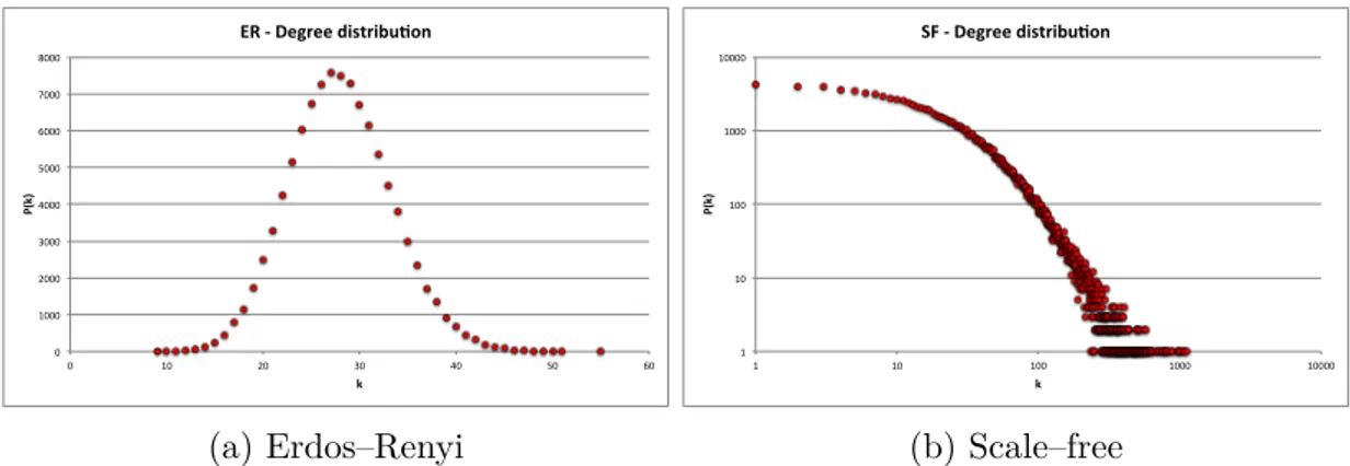
Ta-!" #!!!" $!!!" %!!!" &!!!" '!!!" (!!!" )!!!" *!!!" !" #!" $!" %!" &!" '!" (!" !" #$ % #% &'%(%)*+,**%-./0,.12345% (a) Erdos–Renyi !" !#" !##" !###" !####" !" !#" !##" !###" !####" !" #$ % #% &'%(%)*+,**%-./0,.12345% (b) Scale–free

Figure 3.3: Degree distribution for ER and SF networks ble 3.4 reports the main topological properties of such networks.

Table 3.4: Networks topological parameters

name #nodes #links average degree

ER 100000 1401447 28.028

SF 100000 1394248 27.884

In figure 3.3 the degree distributions of 100K nodes networks is shown. As expected, the ER network (figure 3.3a) exhibits a normal degree distribution, while the SF degree distribution (figure 3.3b) follows a power—law.

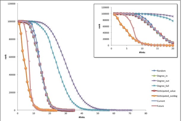
Figure 3.4 reports the rank of me with respect to the number of in-links and steps for all the algorithms presented in the previous subsection. The best rank is represented by the position 1, so at the beginning me has the worst rank, i.e. 100001. The figure shows that

Degree out and Degree full are the worst algorithms in terms of performance. Random,

Degree in, Anticipated value and Current exhibits comparable performance. Despite the

fact Random has the lower computational complexity among the proposed algorithms, it performs as well as more complex algorithms. Future and Anticipated outdeg are the best algorithms when applied to ER networks. Surprisingly Anticipated outdeg performs even better than Future, mainly during the initial part of the attachment process. In fact, as detailed in the figure inset, Anticipated outdeg permits me to rapidly achieve a good rank, even if Future outperforms it after the step number 10. Let’s note, however,

(40)

that the computational complexity of Anticipated outdeg is far less than Future, making the application to very large networks feasible.

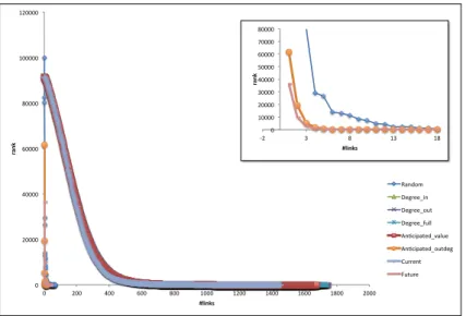
In the figure 3.5 the simulation results for SF network is shown. It’s clear that Random,

Anticipated outdeg and Future outperform the other algorithms proposed in the previous

subsection. As in the case of ER networks, the performance of the Anticipated outdeg algorithm is surprising since its trend is comparable to the more complex algorithm

Future. In addition, Anticipated outdeg allows the node me to reach the best rank in only

18 steps against the 36 required by Future. On the other hand, Random algorithm gets the best rank in 69 steps, that is a very good figure considering the size of the network (100K nodes) and the random selection strategy. This behaviour is probably due to the presence in SF networks of hubs and authority, that play a central role on the dynamic underlying the PageRank evaluation.

!" #!!!!" $!!!!" %!!!!" &!!!!" '!!!!!" '#!!!!" !" '!" #!" (!" $!" )!" %!" *!" &!" !" #$% &'(#$)% +,-./0" 12342256-" 1234225/78" 123422597::" ;-<=6>,82.5?,:72" ;-<=6>,82.5/78.23" @7442-8" A78742" !" #!!!!" $!!!!" %!!!!" &!!!!" '!!!!!" '#!!!!" !" )" '!" ')" #!" !" #$% &'(#$)%

(41)

!" #!!!!" $!!!!" %!!!!" &!!!!" '!!!!!" '#!!!!" !" #!!" $!!" %!!" &!!" '!!!" '#!!" '$!!" '%!!" '&!!" #!!!" !" #$% &'(#$)% ()*+,-" ./01//23*" ./01//2,45" ./01//26477" 8*9:3;)5/+2<)74/" 8*9:3;)5/+2,45+/0" =411/*5" >4541/" !" '!!!!" #!!!!" ?!!!!" $!!!!" @!!!!" %!!!!" A!!!!" &!!!!" B#" ?" &" '?" '&" !" #$% &'(#$)%

Figure 3.5: Heuristics performance on SF network with 100K nodes

3.3 Black Hole Metric

In 3.2’s preamble, some notions concerning node ranking were given in order to describe the problem of best attachment. Particular emphasis was given to the PageRank[52, 53] algorithm, which was used as a basis to devise the various heuristics. In this section, an extension of PageRank named Black Hole Metric [4] will be presented, which aims at solving some outstanding issues of the 18-years old metric.

In the vast amount of digital data, humans have the need to discriminate those relevant for their purposes to effectively transform them into useful information, which usefulness depends on the scenario being considered. For instance, in web searching we aim at finding significant pages with respect to an issued query [38], in an E-learning context we look for useful resources within a given topic [41, 42, 43], or in a recommendation network we search for most reliable entities to interact with [44, 45, 46, 47]. All these situations fall under the umbrella of ranking, a challenge addressed in these years through different solutions. The most well-known technique is probably the PageRank algorithm [52, 53], originally designed to be the core of the Google (www.google.com) web search engine. Since it was published it has been analyzed [102, 98, 103], modified or extended for use in

(42)

other contexts [104, 54], to overcome some of its limitations, and to address computational issues [105, 106].

PageRank has been widely adopted in several different application scenarios. In many of them though, modificiations to the algorithm are applied in order to adapt PageRank to the specific scenario. The Black Hole Metric is a generalization of PageRank whose motivation stems from the concept of trust in virtual social networks. In this context trust is generally intended as a measure of the assured reliance on a specific feature of someone [28, 7, 31], and it is exploited to rank participants in order to discover the best entities that is ”safe” to interact with. This trust-based ranking approach allows to cope with uncertainty and risks [13], a feature especially relevant in the case of lack of bodily presence of counterparts.

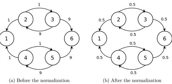
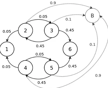
A notable limitation of PageRank when it’s used to model social behaviour, is its inability to preserve the absolute arc weights due to the normalization introduced by the applica-tion of the random walker. In order to illustrate the problem, we introduce a weighted network where arcs model relationships among entities. Entities may be persons, online shops, computers that in general need to establish relationships with other entities of the same type. Let’s suppose to have the network shown in Figure 3.6a, where each arc weight ranges over [0, 10].

Given the network topology, intuition suggests that node 1 would be regarded more poorly compared to node 6 since it receives lower trust values from his neighbors, but, as detailed later, normalizing the weights alters the network topology so much that both nodes are placed in the same position in the ranking. The normalization of the outlink weights indeed hides the weight distribution asymmetry, as depicted in Figure 3.6b. Moreover, PageRank shadows the social implications of assigning low weights to all of

(43)

(a) Before the normalization (b) After the normalization

Figure 3.6: Network with asymmetric trust distribution

a node’s neighbours. If we consider the arcs as if they were social links, common sense would tell us to avoid links with low weight, as they usually model worse relationships. If we look at the normalized weights in Figure 3.6b though, we can see that in many cases, the normalized weight changes the relationship in a counter-intuitive way. Consider the arcs going from node 2 or 4 to their neighbours: we can see that their normalized weights are set to 0.5, which, in the range [0, 1] is an average score. However, the original weight of those links was 1, a comparatively lower score considering that the original range was [0, 10].

The Black Hole Metric copes with the normalization effect and deals with the issue of the skewed arc weights, detalied in subsection 3.3.2. Note that the metric seamlessly adapts to any situation where PageRank can be used, as it’s not limited to trust networks; in the following, they are considered as a simple case study.

(44)

3.3.1 PageRank

Definitions and Notation

In order to better understand the mathematics of the Black Hole Metric, let’s to clarify the notation and provide a few definitions, which are similar to the notations used in the article of PageRank. Let us suppose that N is the number of nodes in the network. We will call A the N × N network adjacency matrix or link matrix, where each aij is the

weight of the arc going from node i to node j. S is the N × 1 sink vector, defined as:

si = ⎧ ⎨ ⎩ 1 if outi = 0 0 otherwise ∀i ≤ N

where outi is the number of outlinks of node i. V is the personalization vector of size

1 × N, equal to the transposed initial distribution probability vector in the Markov chain model PT

0 . While this vector can be arbitrarily chosen as long as it’s stochastic, a common

choice is to make each term equal to 1_/_N. T = 1

N ×1 is the teleportation vector, where the

notation 1N ×M stands for a N × M matrix where each element is 1.

In the general case the Markov chain built upon the network graph is not always ergodic, so it is not used directly for the calculation of the steady state random walker probabilities. As described in [53], the transition matrix M, used in the associated random walker problem, is derived from the link matrix, the sinks vector, the teleportation vector and the personalization vector defined above:

M = d(A + SV ) + (1 − d) T V (3.10)

(45)

the Markov chain theory, the random walk probability vector at step n can be calculated as:

Pn= MTPn−1 (3.11)

the related random walker problem can be calculated as:

P = ( lim n→∞M n)T_P 0 = lim_n→∞(MT)nP0 = M∞TP0 (3.12)

The normalization problem

Let’s calculate the PageRank values of the sample network in Figure 3.6a to highlight the flattening effect of the normalization. By applying the definitions in subsection 3.3.1 the network in Figure 3.6b can be described by the following matrices and vectors:

A= ⎛ ⎜ ⎜ ⎜ ⎜ ⎜ ⎜ ⎜ ⎜ ⎜ ⎜ ⎜ ⎝ 0 0 0 0 0 0 0.5 0 0.5 0 0 0 0 0.5 0 0 0 0.5 0.5 0 0 0 0.5 0 0 0 0 0.5 0 0.5 0 0 0 0 0 0 ⎞ ⎟ ⎟ ⎟ ⎟ ⎟ ⎟ ⎟ ⎟ ⎟ ⎟ ⎟ ⎠ S= ⎛ ⎜ ⎜ ⎜ ⎜ ⎜ ⎜ ⎜ ⎜ ⎜ ⎜ ⎜ ⎝ 1 0 0 0 0 1 ⎞ ⎟ ⎟ ⎟ ⎟ ⎟ ⎟ ⎟ ⎟ ⎟ ⎟ ⎟ ⎠ V = P₀T = 1 6 · 11×6 T = 16×1