Facoltà di Ingegneria
Laurea Specialistica in Ingegneria dell’Automazione
Tesi di laurea
Candidato:
Giulio Telleschi
Relatori:
Prof. Andrea Caiti
-
Università di Pisa
Prof. Monique Chyba
-
University of Hawaii
A
N
EW
A
PPROACH
T
O
M
ODELING
M
ORPHOGENESIS
U
SING
C
ONTROL
T
HEORY
Sessione di Laurea del 11/05/2012
Archivio tesi Laurea Specialistica in Ingegneria dell’Automazione Anno accademico 2011/2012
2
A
CKNOWLEDGMENTS
First and foremost, I would like to thank Professor Andrea Caiti for the great opportunity he offered me and for his constant enthusiasm supporting my work, and Dr. Monique Chyba for letting me join her research group, motivating me as no one else did before and have a unique chance to grow professionally. Without them, this thesis would not have been possible.
I would also like to thank John Rader for his guidance and for the fair team work we made together, and Aaron Tamura Sato for his technical support. Finally, I would like to thank the Departments of Mathematics and of Mechanical Engineering at the University of Hawaii, in the person of Dr. M. Kobayashi, for treating me as a peer and giving me a lot of gratification.
Ringrazio la mia famiglia, in ogni sua colorata declinazione, per il supporto incessante in tutti gli anni di studi e per il costante incoraggiamento che mi ha fornito anche nei momenti più difficili; Azzurra per avermi accompagnato in un’altra importantissima tratta di questo straordinario percorso e tutti gli amici, even the
3
A chi non c’è più,
perché ci sarà sempre.
4
A
BSTRACT
It has been proposed that biological structures termed fractones may govern morphogenic events of cells; that is, fractones may dictate when a cell undergoes mitosis by capturing and concentrating certain chemical growth factors created by cells in their immediate vicinity. Based on this hypothesis, we present a model of cellular growth that incorporates these fractones, freely-diffusing growth factor, their interaction with each other, and their effect on cellular mitosis. The question of how complex biological cell structures arise from single cells during development can now be posed in terms of a mathematical control problem in which the activation and deactivation of fractones determines how a cellular mass forms. Stated in this fashion, several new questions in the field of control theory emerge as the configuration space is constantly evolving (caused by the creation of new cells), and thus cannot be analyzed using traditional techniques of control theory. We present this new class of problems, as well as an initial analysis of some of these questions. Also, we indicate an extension of the proposed control method to layout optimization.
5
S
OMMARIO
Recenti studi hanno evidenziato l’esistenza di strutture biologiche, chiamate frattoni, in grado di controllare la morfogenesi delle cellule. I frattoni quindi, assorbendo i fattori di crescita prodotti dalle cellule nelle loro immediate vicinanze, danno l’input affinché le cellule procedano alla mitosi. In base a queste ipotesi, proponiamo un modello di crescita cellulare che include i frattoni, i fattori di crescita liberi di diffondersi nello spazio, le interazioni che ne scaturiscono e il conseguente effetto sulla duplicazione cellulare. Possiamo dunque formulare in termini matematici e di controllo il problema della formazione di una struttura biologica complessa composta dalle cellule per la quale l’attivazione e la disattivazione dei frattoni determina lo sviluppo della struttura. Definendo il problema in questi termini, sorgono molte domande nel campo della teoria del controllo poiché lo spazio di operativo è in continua evoluzione (a causa della creazione di nuove cellule) e quindi non può essere condotta un’analisi mediante le tradizionali tecniche della teoria del controllo. Attraverso questo studio, presentiamo una nuova classe di problemi unitamente ad una prima analisi delle domande che ne scaturiscono. Infine, è mostrata una possibile estensione del modello all’ottimizzazione di layout.
6
L
IST
O
F
C
ONTENTS
Introduction ... 9
Motivation ... 15
1. One Dimensional Model ... 20
2. Two Dimensional Model... 24
2.1 Discretization of the problem... 24
2.2 Diffusion of growth factor ... 27
2.3 Mitosis ... 33
3. Theoretical Questions and Results ... 42
3.1 Existence of solutions ... 44
3.2 Uniqueness of solutions ... 45
3.3 Notion of distance between configurations of cells ... 46
4. Model Improvements to fit Biological Experiments ... 61
4.1 Growth factor diffusion speed ... 61
4.2 Growth factor redistribution ... 64
4.3 Growth factor production ... 67
4.4 Fractone activation ... 68
5. MATLAB Code Explanation ... 77
5.1 Ambient, variables and subspaces definition ... 77
5.2 System dynamics ... 78
5.3 Mitosis ... 78
5.4 Data plotting... 79
6. Application To Layout Optimization ... 80
6.1 MATLAB code explanation ... 81
7. Future Work ... 87
8. Conclusions ... 89
7
L
IST
O
F
F
IGURES
Figure 1 - Fractones are extracellular matrix structures. ... 11
Figure 2 - Characterization of fractones in the mouse ... 17
Figure 3 - Discretisation of a fractone map ... 24
Figure 4 - Discretization: Free(t) ... 27
Figure 5 - Discretization: Fract(t)... 27
Figure 6 - Discretization: Cell(t) ... 27
Figure 7 - Discretization: Conf(t) ... 27
Figure 8 - Free diffusion ... 29
Figure 9 - Perturbed diffusion ... 32
Figure 10 - Distance distribution: an example ... 37
Figure 11 - Deformation algorithm ... 40
Figure 12 - First and last frame of a simulation with multiple cells and fractones .... 41
Figure 13 - Existence of solutions ... 44
Figure 14 - Uniqueness of solutions ... 45
Figure 15 - Cell (grey) and A Cell (light blue) discretized as circles ... 47 B Figure 16 - Walks between cells. ... 50
Figure 17 - (a) 1-connected cell space, (b) minimally 3-connecrted cell space... 51
Figure 18 - Distance from a configuration... 52
Figure 19 - Possible configuration at same Hausdorff distance... 58
Figure 20 - 2-unit channel between adjoining cells ... 63
Figure 21 - 2-unit channel between adjoining cells, three dimensional simulation ... 63
Figure 22 - Channel free from GF after mitosis... 65
Figure 23 - Growth factor redistridution as a pressure wave ... 66
Figure 24 - Growth factor production ... 68
Figure 25 - Fractone activation/deactivation ... 70
Figure 26 - Fractone not associated to a cell ... 71
Figure 27 - A fractone resulting in an obstacle ... 72
Figure 28 - An exhaustive simulation ... 76
Figure 29 - Application to layout optimization ... 85
8
L
IST OF
T
ABLES
Table 1 - Mathematics Arising from Biological Problems ... 14 Table 2 - D: distance distribution as measured from the "mother" cell ... 36 Table 3 - Parameters for GF production ... 67
9
I
NTRODUCTION
All vertebrate animals, including humans, produce new neurons and glia (the two primary specialized cell types of the brain) throughout life. Neurons and glia derive from neural stem cells, which reside, proliferate, and differentiate in specialized zones termed niches. Neural stem cells proliferate extensively during development and progressively generate the brain, a phenomenon named neurulation, or brain morphogenesis. Interestingly, neural stem cells exist and continue to generate neurons and glial cells after birth and throughout adulthood in very restricted niches, primarily the walls of the lateral ventricle. What are the mechanisms that control neural stem cell proliferation and differentiation? Neural stem cells and their progeny respond to growth factors, endogenous signaling molecules that circulate in the extracellular milieu (in between cells).
The process of neurulation and subsequent events of the brain’s formation involve multiple growth factors that induce proliferation, differentiation, and migration of cells. The distribution and activation of these growth factors in space and time will determine the morphogenic events of the developing mamalian brain. However, the process organizing the distribution and availability of growth factors within the neuroepithelium is not understood. Structures, termed fractones, directly contact neural stem and progenitor cells, capture and concentrate said growth factors, and are associated with cell proliferation ( [1], [2], [3] ). Hence, our hypothesis is that fractones are the captors that spatially control the activation of growth factors in a precise location to generate a morphogenic event.
Inspired by these biological discoveries, we propose to develop and analyze a mathematical model predicting cell proliferation from the spatial distribution of fractones. Dynamic mathematical modeling, i.e. models that represent change in rates over time, serves several purposes [4]. Using computer simulations, by mimicking the assumed forces resulting in a system behavior, the model helps us to understand the nonlinear dynamics of the system under study. Such approach is especially well suited
10 for biological systems whose complexity renders a purely analytical approach unrealistic. Moreover, it allows us to overcome the excessively demanding purely experimental approach to understand a biological system. Our primary goal in this paper is to develop a model that contains the crucial features of our hypothesis and, at the same time, is sufficiently simple to allow an understanding of the underlying principles of the observed system.
We propose to model this biological process as a control system, the control depicting the spatial distribution of the active fractones. This is a novel approach with respect to the most commonly reaction-diffusion models seen in the literature on morphogenesis, however it is not that surprising. Indeed, control theory is instrumental to overcome many challenges faced by scientists to design systems with a very high degree of complexity and interaction with the environment ( [5], [6], [7] ). Examples of its applicability in physical and biological systems are numerous ( [8], [9] ).
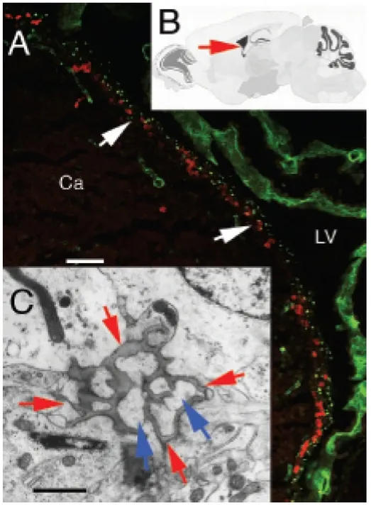
11 Figure 1 - Fractones are extracellular matrix structures associated with proliferating cells in the
neurogenic zone (neural stem cell niche) of the adult mammalian brain.1
1
(A) Visualization of fractones (green, puncta, arrows) by confocal laser scanning microscopy in the primary neurogenic zone of the adult mouse brain, i.e. the wall of the lateral ventricle (LV) at the surface of the caudate nucleus (Ca). Each green puncta is an individual fractone. The red puncta indicate proliferating neural stem cells and progenitor cells immunolabeled for the mitotic marker bromodeoxyuridine. Stem cells and their progeny proliferate next to fractones (arrows). (B) Location of the confocal image A (arrow) in a schematic representation of the mouse brain (cut in the sagittal plane). (C) Visualization of an individual fractone by transmission electron microscopy (dark-grey structure indicated by the four red arrows. The processes of neural stem cells and of their progeny, which appear light-grey (blue arrows) are inserted into the folds of the fractone. Scale bars. A: 50 μm; C: 1 μm.
12 Historical Usage of Mathematics in Biology
The history of mathematics used to solve problems arising from biology dates back several hundred years to the times of Bernoulli and Euler. Prior to the mid-1900s, though, biology served primarily as the inspiration to understanding larger problems rather than as a practical field to be studied under the rigors of applied mathematics. Many problems in the field, even simplified with strong assumptions and in their least-complex forms, were unable to be solved using traditional techniques of mathematicians due to their complexity. Researchers of the day were either forced to pay understudies to perform hundreds, perhaps thousands, of hand calculations, or they would make drastic simplifications of their models merely to gain insight into the behavior of the system, and, as a consequence, many would make incorrect conclusions when compared versus real-world data. However, at times, some models were found to be accurate when compared to known data, and thus were accepted as theory (this is most likely due to acceptable simplifications, those not significant to the model as a whole).
Once the mid-20th century arrived, and with it the advent of the computer, researchers finally had the luxury of being able to analyze complex systems without unnecessary simplifications. And with the creation of the personal computer and modern computational software (as well as the internet and supercomputing clusters) in the 1980s, scientists and researchers could now fully model the most complex system without any necessary simplifications and can find solutions (albeit numeric) for a variety of problems.
Much of what has been attempted to solve or has been solved using mathematics in the field of biology is summarized in Table 1.
Historical Usage of Control Theory in Biology
The appearance and usage of control theory in the field of biology is a relatively new idea, dating back only a few decades. The first real evidence of the usage of control theory to understand a biological process originates with Norbert Wiener [10], who developed many of the ideas of feedback and filtering in the early 1940s in collaboration with the Harvard physiologist Arturo Rosenblueth, who was, in turn, heavily influenced by the work of his colleague Walter Cannon [11], who coined the
13 term homeostasis in 1932 to refer to feedback mechanisms for set-point regulation in living organisms. Rudolf Kalman [12] often used biological analogies in his discussion of control systems theory, and so did many other early researchers. Modern biological control, enveloped in the more general field of systems biology, emanates from the work of Ludwig von Bertalanffy [13] with his general systems theory. One of the first numerical simulations in biology was published in 1952 by the British neurophysiologists and Nobel prize winners Alan Hodgkin and Andrew Huxley [14], who constructed a mathematical model that explained the action potential propagating along the axon of a neuronal cell. Also, in 1960, Denis Noble [15], using computer models of biological organs and organ systems to interpret function from the molecular level to the whole organism, developed the first computer model of the heart pacemaker. The formal study of systems biology, as a distinct discipline, was launched by systems theorist Mihajlo Mesarovic in 1966 with an international symposium at the Case Institute of Technology in Cleveland, Ohio entitled “Systems Theory and Biology” [16].
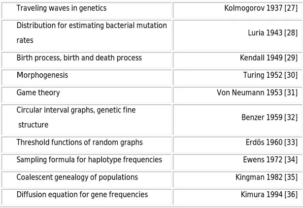
Subject Reference
Spread of diseases Bernoulli 1760 [17] Fluid mechanics of blood flow Euler 1760 [18] Age structure of stable populations Euler 1775 [19] Logistic equation for limited population
growth Verhulst 1838 [20]
Branching processes, extinction of family
names Galton 1889 [21]
Correlation Pearson 1903 [22] Markov chains, statistics of language Markov 1906 [23] Hardy-Weinberg equilibrium in population
genetics Hardy 1908 [24]
Dynamics of interacting species Lotka 1925 [25]; Volterra 1931 [26]
14
Traveling waves in genetics Kolmogorov 1937 [27] Distribution for estimating bacterial mutation
rates Luria 1943 [28]
Birth process, birth and death process Kendall 1949 [29] Morphogenesis Turing 1952 [30] Game theory Von Neumann 1953 [31] Circular interval graphs, genetic fine
structure Benzer 1959 [32] Threshold functions of random graphs Erdös 1960 [33] Sampling formula for haplotype frequencies Ewens 1972 [34] Coalescent genealogy of populations Kingman 1982 [35] Diffusion equation for gene frequencies Kimura 1994 [36]
Table 1 - Mathematics Arising from Biological Problems
The field of systems biology is large and encompassing, so much so that it, at times, is hard to define what is and is not part of the field. However, the kinds of research and problems that have laid the groundwork for establishing the field are as follows:
complex molecular systems, such as the metabolic control analysis and the biochemical systems theory between 1960-1980 ( [37] , [38] )
quantitative modeling of enzyme kinetics, a discipline that flourished, between 1900 and 1970 [39]
mathematical modeling of population growth simulations developed to study neurophysiology control theory and cybernetics [40]
Some recent problems approached by those studying control theory in the field of biology have been to model, among others:
internal workings of the cell
15 cell signal transduction processes
neural pathways
regulation versus homeostasis
RNA/DNA transcription with an emphasis on mutation gene function and interactions.
The breadth and variety of problems that can be modeled using control theory runs the gamut, from the molecular through the microscopic up to the macroscopic. Many areas of biology have been affected by many areas of mathematical science, and the challenges of biology have also prompted advances of importance to the mathematical sciences themselves. The rapidly developing field of systems biology (the merging of biology, physics, engineering, and/or mathematics) is tremendously exciting, and full of unique research opportunities and challenges, especially for the application of control theory.
Motivation
This research has been held towards three different fields of science: biology, mathematics and engineering.
Biological Motivation
A fundamental problem is to understand how growth factors control the topology of cell proliferation and direct the construction of the forming neural tissue. It has been demonstrated that extra-cellular matrix (ECM) molecules strongly influence growth factor-mediated cell proliferation. ECM proteoglycans can capture and present growth factors to the cell surface receptors to ultimately trigger the biological response of growth factors. Hence, by building a model that incorporates the most important features of the biological system, we attempt to simulate how this occurs to give more insight into how structure of biological systems takes shape under the assumption that it is driven by the presence of growth factors and activation by ECM molecules, particularly fractones.
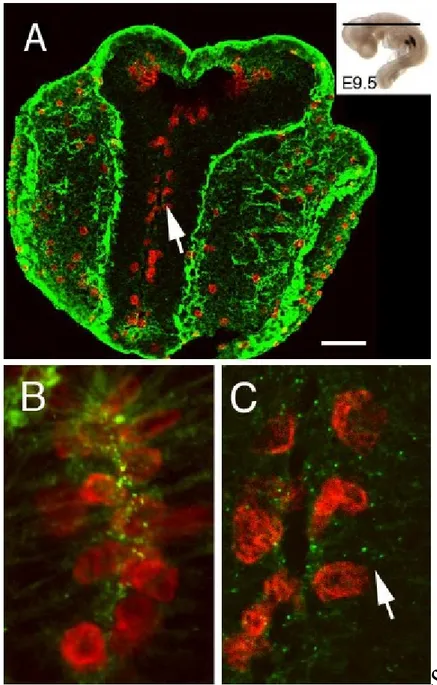
16 F.Mercier and his collaborators have discovered ECM structures that are associated with proliferating cells in the stem cell niche of the adult mammalian brain ( [1], [2], [3]). These structures, termed fractones, hold a high potential as captors of mitotic and neurogenic growth factors. In Figure 2 (A) we have a laser scanning confocal microscopy image showing the section of the whole head of an E9.5 embryo (9.5 days post-coitum). Proliferating neuroepithelial cells were visualized by phosphorylated histone-3 (PH3, a marker of mitosis) immunofluorescence cytochemistry (red). The extracellular matrix material was revealed by immunoreactivity for laminin, a ubiquitous glycoprotein found in basement membranes and fractones. However, fractones are too small to be visualized at this level of magnification. Note that cells proliferate near the lumen of the forming cavity (arrow, neural groove). The plan of section is indicated in the inset. (B) High magnification confocal microscopy field showing proliferating neuroepithelial cells (PH3 immunoreactivity, red) associated with fractone (green punctae) at E8.5. (C) Magnification of the area indicated by an arrow in A showing that neuroepithelial cells also proliferate (red) next to fractones (green punctae, arrow) at E9.5.
During our research, we analyzed a space in which there exist three unique components: fractones, cells/holes, and growth factors (GFs) that cells produce. The initial configuration is (at least) one cell and one associated fractone. The cells produce growth factors on a fixed, regular time interval and in discrete amounts. The time at which an individual cell produces growth factor, however, may be different from any other cell (depending on when each cell entered the system). Once produced, the GFs diffuse radially away from the cell into the extra-cellular diffusion space that occurs between cells. The GFs do not chemically interact with each other, and they are actively trapped by a fractone when significantly close. Once a fractone has absorbed enough GF beyond some threshold, it sends a signal to the associated cell(s) to undergo mitosis. A hole is similar to a cell, except that it does not produce GF. In fact, a hole can be thought of as a wall, a non-interacting object that the system evolves around.
17 Figure 2 - Characterization of fractones in the mouse neuroepithelium during brain morphogenesis
Mathematical Motivation
The classical models attempting to describe morphogenesis are based on Reaction-Diffusion (RD) equations developed in Turing’s “Morphogenesis” [30]. Although Turing made a great attempt to mathematically portray morphogenesis, his work is not an adequate model to describe the system given new discoveries and developments since the 1950s. With his model, Turing was describing how reactive chemicals present
18 in a static, living structure interact in a continuous medium (a skin tissue, for example) via diffusion (and, surprisingly, form wave-like patterns). For the system we are describing, reaction-diffusion equations cannot be used to study the mechanisms of morphogenesis during development as the growth factors are non-interacting.
Turing’s hypothesis came from the simplistic approach that diffusion and subsequent chemical reactions of an activator/inhibitor pair of chemicals are what drive pattern formation, leading to the following equations for a one dimensional model:
1 2 1
, 1, ,r r r r r
X f X X X X for r N
where N represents the number of cells in the system, X is the concentration of morphogens and is a diffusion constant.
Since growth factors are non-reactive, we should not use the reaction function f X
r
. To expand this model to higher dimensions, the equation must accommodate more neighbors. Thus, the 2D diffusion equation is:
( , )i j ( , )i j ( 1, )i j ( 1, )i j ( ,i j 1) ( ,i j 1) 4 ( , )i j
X f X X X X X X
Based on the hypothesis of ( [1], [2], [3] ), morphogenesis involves the capture and activation of growth factors by fractones at specific locations according to a precise timing. Also, Turing’s assumption of unchanging state space (i.e. there is no growth, or the cells do not replicate) is not applicable to our model since, as cells replicate, the system of equations describing the “diffusion-trapping” model grows by one equation for every new cell produced. This adds mathematical complexity to the problem in that the system of equations governing the model are increasing in number. As mentioned before, the fractones influence GF-mediated cell proliferation, which is also a sign that Turing’s model will not suffice, as there is no mechanism in the reaction-diffusion equations for structures with this type of action. Moreover, the distribution of fractones is constantly changing duringdevelopment, reflecting the dynamics of the morphogenic events. Therefore, the organizing role of fractones in morphogenesis must be analyzed by an alternative mathematical model.
19 Engineering Motivation
As part of engineering design, layout optimization plays a critical role in the pursuit of optimal design. Layout optimization aims at finding the optimum distribution or layout of material within a bounded domain, called the design domain, that minimizes an objective or target function, while satisfying a set of constraints (see the recent monograph and reviews ( [41], [42] , [43])).
Existing topology optimization methods rest on mathematical foundations (see, for example, [41], [44] ). And mathematically, the search space, where the optimization layout is defined, is a topological vector space of infinite dimension - usually a Sobolev space [44]. In practice, however, computational methods used to solve layout optimization can only store and compute finite amount of data. This limitation forces any numerical optimization methods to rely on approximations of the search space and of the admissible topology configurations. The popular SIMP method [41], for example, models the search space as discrete functions on the discretized design domain. In other words, each point represents the "pixel" of the desired blueprint of the optimal design. As a consequence, a good resolution of the design may require a large number of pixels, and these pixels model both void and solid regions.
Similarly to our computational methods, natural systems are also restricted to a finite encoding: the DNA. However, natural systems have devised a strikingly different solution to the finitude problem, where the DNA encodes a developmental program that when "compiled and executed" performs a sequence of tasks that develops the final structure in stages. The results are patterned, complex, and multi-scaled structures that perform multiple task functions and are generically resistant to damage.
The goal of this research will be to develop a cellular proliferation process that mimics the developmental stages of natural organisms. These laws can be evolved to respond to desired requirements, and thus be used to search for high-performing engineering layouts.
20
1. O
NE
D
IMENSIONAL
M
ODEL
We first study a simple case in order to understand how it is possible to model such a biological process, defining control inputs and basic rules that will be developed further on. Our initial assumption is that the geometric configuration of the cells is a ring of at least 3 cells. For the ring of cells, the topology is unaffected, as only the radius increases. The model is a control system that will predict the dynamic distribution of fractones (and attached cells) and their contribution to the morphogenesis process. The system will be modeled as a control system to incorporate dynamic changes in the distribution of fractones among the cells. In general, the state space of our control system represents the concentrations of a given number of growth factors at a precise location in a given configuration of cells. Mathematically, these systems are described by a differential equation of the form:
( ) ( ( ), ( )), ( )
x t f x t u t x t M (1.1) where M is a n-dimensional smooth manifold, x describes the state of the system and
:[0, ] m
u T U is a measurable bounded function called the control. Despite the fact that the field of control theory covers such a broad range, the biological process that we are analyzing presents a completely new challenge from the control theory point of view. We are primarily concerned with the affine control system:
0 1 ( ) ( ( )) ( ( )) ( ), ( ) m j j x t F x t F x t u t x t M
(1.2)where the vector field F0 is referred to as the drift and the Fjs are referred to as the control vector fields (m represents the number of available inputs, in particular if mn
we say that the system is underactuated). Let us consider the state space of our control system to be the concentrations of a given number of growth factors at a precise location in a given configuration of cells. The drift vector field will represent the diffusion property of the growth factors under the condition that no fractone is active
21 while the control vector fields represent the impact that a fractone will have on the diffusion process once it is activated. The spatial distribution of the fractones is governed by the control function:
0 if fractone inactive ( ) 1 1 if fractone active i u t for i m (1.3)
Assume that we have k growth factors diffusing among the cells; we call them Xk. Each growth factor has its own diffusion rate that will be denoted byk and 0 k
i
X represents the concentration of the growth factor Xk in the ith−cell. Note that 0th−cell is synonymous with the Nth−cell, where N represents the total number of cells. Now, we describe the system for a single growth factor. The component i of the drift vector field
,0 ( ( )) k k F X t is: ,0 1 1 ( ( )) ( 2 ) k k k k k k i i i F X t X X X (1.4)
This equation comes from Turing, and is modified to reflect that there are no cross-reaction terms (since the GFs are non-interacting) and the presence of a diffusion constant for each respective growth factor. The system X tk( )Fk,0(X tk( )) represents pure diffusion.
Now, as t , such a system tends to the steady state solution in which the
concentration of growth factor is identical in each cell. However, once a fractone associated to the ith-cell is activated, the diffusion process is perturbed; there is diffusion from the neighboring cells to the ith-cell but diffusion from the ith-cell to its neighboring cells is prevented. In other words, the fractone associated to the ith-cell acts as a captor of growth factor. In terms of the equations describing the system, when the fractone associated to the ith-cell is activated, only the component ui of the control is turned on (taking the value 1) and the control vector field Fk i,(X t describes the new diffusion k( )) process. By construction, Fk i,(X t only affects the diffusion of the (i − 1)k( )) th, ith, and (i + 1)th-cells. Now, we introduce the exchanging function that dictates whether neighboring cells give growth factor to one another by:
( ) ( k( ) k( ))( k( ) k( ))
st s t s t
22 where we define: 0, 0 ( ) 1, 0 if z H z if z (1.6)
With these notations, we have:
, ,0 1, 1, , 1 1, 1 , 1 1, 1 ( ( )) ( ( ( ))) ( ( )) ( ) ( ( )) ( ) k i k k k i k i i i i k i k k k i k i i i i k i k k k i k i i i i F X t H H F X t F X t H X X F X t H X X (1.7)
and all the other components of the control vector field Fk i,(X t are zero. If we k( )) consider multiple growth factors diffusing among the cellular structure, we must take them into account via superposition of the system and implementation of a hierarchical system to describe the affinity of a given fractone with a certain type of growth factor. This adds complexity to the system, but it is a straightforward extension.
From the point of view of control theory, system (1.2) falls into the classical theory of control systems since it is affine and fully actuated (a fractone can potentially be activated in any cell). All the components of the control are piecewise constant functions that take their values from the set {0, 1} and, given an initial distribution of fractones, it is trivial to produce a control to reach a prescribed final distribution of cells. However, to achieve our goal, we must develop a more realistic model to incorporate the activation of the growth factors that will dictate the multiplication of cells.
To refine the model we’ve developed thus far, we assume that once a given concentration for the growth factor k
X is reached at a fractone (or, equivalently, a captor), it releases the information to the attached cell to duplicate, and the concentration of growth factor in the cell drops to a lower amount. When this situation manifests, the number of cells in the ring grows from N to N+1. This implies that the state space on which our biological control system is defined is dynamic, as its dimension transforms with the cells duplication. Based on how we perceive the system to function, the control system that models it is as follows:
( ) 0 1 ( ) ( ( )) ( ( )) ( ), ( ) N t j j x t F x t F x t u t x t M
(1.8)23 where M(t) is now a space whose dimension and topology varies with time. In a simplified way, this corresponds to saying that the number of cells grows, which is reflected in the equation by the introduction of N(t). Also, the domain of control now varies since fractones can potentially become active in the new cells.
24
2. T
WO
D
IMENSIONAL
M
ODEL
We need to define the relevant components for the biological process under consideration, and their discretization: the ambient space, the cells, the bones and the fractones.
2.1 Discretization of the problem
The ambient space in which the morphogenic events take place is assumed to be a compact subset of 2
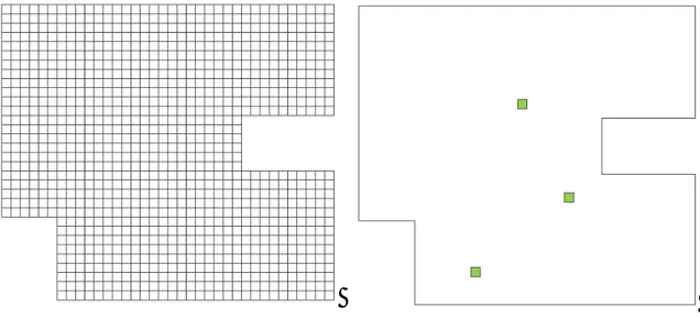
and, for simplicity, we assume the ambient space is fixed. We denote by M a discretization of the ambient space (using for instance discretization by dilatation or Hausdorff discretization, see [45] and Figure 3).
25 So, in the sequel, M is identified to a subset of 2. The precision of the discretization is initially set by the user but eventually will be determined by the experimental biological maps. To avoid any confusion with the biological cells, in the rest of this thesis, we call a cell of our discretization a unit and we identify each unit to an ordered pair of integer
i j,
. The origin unit of our discretization is chosen arbitrarily and will be identified to
0, 0
. We assume that the boundary of the ambient space in which the biological process takes place is fixed but our definitions allow for boundaries that vary with time as well.For simplicity will consider a rectangular ambient space, but we can easily modify its shape by modeling bones. Intuitively, in our discretization, a bone will be modeled as a region not accessible to our system: we can imagine it as an hole (inside the ambient space) or a wall (if it changes the boundary of the ambient space). Referring to the proper definition of M, bones are useful to design the shape of the ambient space but once we get the desired conformation, bones will not show up in our model. There is no restriction in the use of bones because they are defined unit by unit, in order to create any shape needed.
The morphogenic event will start from an initial configuration of cells immerged in what we call the ambient space. Growth factors diffuse within the ambient space but can’t go through cells. A cell border is modeled as a wall for the growth factors that are outside the cell but we’ll see further on that the cell will be able to produce growth factors that will diffuse in the ambient space. We assume that the space between the cells account for 20% of the total space occupied by the cells. This is reflected in our discretization by representing a cell as a square composed of 81 units (i.e. a 9 by 9 square) 2, while the “in-between cells” space is represented by single rows and unit-columns. Notice that at this stage of the work it is an arbitrary choice and it will be straightforward to adjust it to reflect the observations from the experimental maps. We assume the cells to be vertically and horizontally aligned.
2
From a purely theoretical point of view, there are many ways that we can represent the cells in the ambient space. Indeed, we can make the assumption that they are all circular and have the same dimension or that their shape differs in size and form. Notice that, from a practical point of view, the shape and size of the cells of the initial configurations will be given by the experimental map and its discretization. To write the dynamic model of our biological process we only assume that the size and shape of all cells are identical.
26 Finally, in our discretization, a fractone is represented as one unit. Growth factors are attracted by fractones and are stored in them.
The three important spaces to take into account into our dynamical system are: the space filled with cells, the space in which the growth factors diffuse and finally the space filled with the fractones. Those objects are defined in the following definitions. We denote by Cell t( )the configuration of cells in the ambient space at a given time t ,
and we call it the cell space. It is a closed subset of the ambient space and is identified in the sequel to a subset of M.
The diffusion space at time t , denoted by Diff t( ), represents the space in which growth factors are diffusing. It is the complement of the cell space in the ambient space and its discretization is identified to M Cell t\ ( ). At each time t , the diffusion space is split
into two components, the free diffusion space Free t( ) where the growth factors diffuse freely, and the fractone space, Fract t( ), where the diffusion is perturbed. The data of
( )
Cell t , Free t( )and Fract t( )forms what we call the configuration space at time t , and
we denote it by Conf t( ).
Note that M Cell t( )Diff t( ) and Diff t( )Fract t( )Free t( ).
Let M t( ) be one of the spaces defined above. We define the dimension of the space M at time t as the number of indices ( , )i j such that ( , )i j M t( ) where M t( ) has been identified to its discretization.
Topologically, we can interpret the above definitions as follows: we can visualize the configuration space at a given time t as a compact subset of 2
with holes depicted by the cells. On a given discretization of this topological space (varying with time), we will model the diffusion of growth factors (which is perturbed at the location of a fractone). Finally, we will incorporate into our model the mechanisms that allows duplication of cells named mitosis.
An example of how the discretization process takes place is shown from Figure 4 to Figure 7, where we can see the diffusion space (highlighted by the grid showing free units) of complex shape, thank to the use of bones, plus cells (in blue) and fractones (green units).
27 Figure 4 - Discretization: Free(t) Figure 5 - Discretization: Fract(t)
Figure 6 - Discretization: Cell(t) Figure 7 - Discretization: Conf(t)
2.2 Diffusion of growth factor
For simplicity, we assume the diffusion of a unique type of growth factor and equal sensitivity of the fractones with respect to that growth factor. However, our model will be developed such that expanding to several types of growth factors and varying fractone sensitivity to respective growth factors can be added in a straightforward way. The state space is defined at each time t as the concentration of growth factor in each
28
( )
M t . More precisely, since there is a one-to-one correspondence between units and ordered pairs of integer, we have:
DEFINITION - Let ( , )i j Diff t( ). At each time t , we introduce the concentration of
growth factor in unit ( , )i j that we denote by Xi j, ( )t . The state space M t( ) at time t is then M t( ) dim(0 Diff t( )).
Assume at first that there is no cells and no fractones. Therefore, the growth factors diffuse freely in the ambient space. We denote by the diffusion parameter associated to the considered growth factor, and in order to accurately describe the mechanism we introduce
0,1 , 0, 1 , 1, 0 ,
1, 0
.Pure dissipation is then described by:
0 ( ) ( ( ))
X t F X t (2.1)
where the components of X t( )are given by Xi j, ( )t which represents the quantity of growth factor in unit ( , )i j at time t as described chapter 1, and, assuming diffusion
occurs between a unit ( , )i j and its four neighbors, we have:
, , , ( , ) ( ) ( ( ) ( )) i j i k j l i j k l X t X t X t
(2.2)for ( , )i j Diff t( ), see Figure 8.
Assume now that a cell forms in the ambient space. The cell therefore becomes an obstacle to the diffusion process. Mathematically, rather than looking at a cell as an obstacle, we identify the cell to a hole in a topological space. The hole, depicting the location of the cell, insures that the diffusion of the growth factor takes place in the diffusion space only. By doing so, we do not have to perturb the diffusion process, instead we continuously modify the topological space in which the diffusion process takes place.
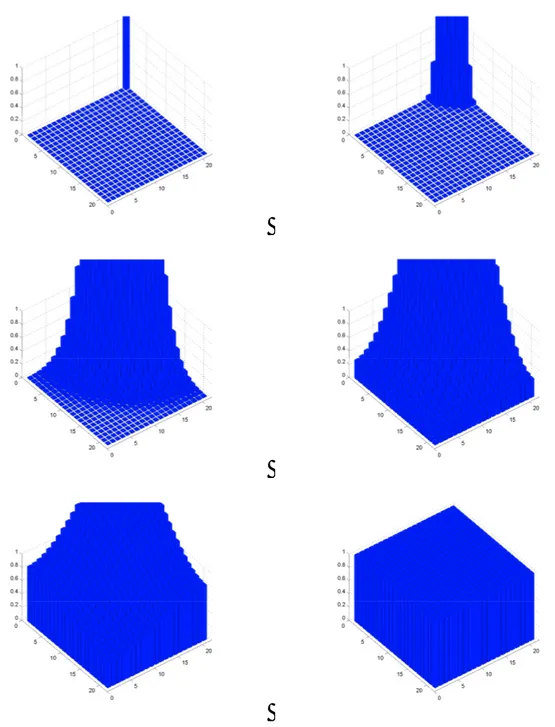
29 Figure 8 - Free diffusion
Let us describe the new state space on which the diffusion process takes place. Assume the cell is centered at unit ( , )a b . This means that at the time t at which the cell
formed, the diffusion space Diff t( )ItJt transforms into a new free diffusion space t t
I J from ItJt\
a4,,a4
b4,,b4
,we assume it is instantaneous with no loss of generality. Notice that, since several cells might be forming at the same30 time, the topological changes in the configuration space will reflect all the created holes. We then have: , , , ( , ) ( , ) ( ) ( ) ( ( ) ( )) i j i k j l i j k l i k j l Diff t X t X t X t
(2.3) for ( , )i j Diff t( ).Finally, we need to model how fractones perturb the diffusion. As mentioned before, a fractone is represented as a one unit ( , )i j of our discretization. The hypothesis is that the fractones store the quantity of growth factors that they capture, and that this quantity becomes unavailable to the diffusion process. To reflect the biological hypothesis that fractones are produced and then disappear, we introduce the following definitions.
DEFINITION - To each unit ( , )i j we associate what we call a passive fractone. A passive fractone at time t belongs to Free t( ). An active fractone at time t is defined
as a unit that belongs to the set Fract t( ). An active fractone is one that acts as a captor for the diffusion process.
The biological translation of this definition goes as follow. A passive fractone corresponds to the situation such that either no fractone is associated to the unit or one is currently produced but is not yet part of the biological process. In other words, in our representation it can be seen that Free t( ) is the set of passive fractones at time t . An
active fractone is one that acts as a captor for the diffusion process.
Assume now that there is an active fractone ( , )i j . Then there is perturbation to the diffusion process as follows. We introduce a control function ( ) ( , ( ))
0,1 It Jti j
u t u t defined on a time interval
0,T
, with T representing the duration of the cascade of morphogenic events under study. When a fractone is active at time t , the component, ( )
i j
u t of the control is turned on to 1 while it is set to zero for a passive fractone. The active fractone store the current quantity of growth factors available in unit ( , )i j and acts as captor for the diffusion process. In other words, diffusion from an unit
31
( , )i j Fract t( )to its neighbors is prevented. To represent this perturbed diffusion process, we define a control system:
0 ( , ) ( , ) ( , ) ( ) ( ) ( ) i j ( ) i j ( ) i j Diff t X t F X t F X t u t
(2.4)where X t( )is the state variable and denotes the concentration of growth factor in the diffusion space Diff t( )ItJt at time t , the drift vector field 0
F is given by (2.3) and represents the regular diffusion of growth factors taking place in the free diffusion space, and finally the control vector fields perturb the regular diffusion to account for the possible presence of active fractones. More precisely, we have under the assumption that ( , )i j is an active fractone:
( , ) , , ( , ) ( , ) ( ) ( ) ( ) i j i j i j k l i k j l Diff t F X t X t
(2.5)
( , ) , , ( , ) ( ) ( ), ( , ) ( ) i j i k j l i j k l F X t X t for i k j l Diff t (2.6)Those equations reflect the fact that the quantity of growth factor in an active fractone become invisible to the diffusion process. Once the stored quantity reaches a given threshold, the fractone signals to the cells that mitosis can occur. Moreover, a key element in our hypothesis is that the spatial distribution of fractone varies through the sequence of morphogenic events. The role of the function u ( ) introduced in (2.4) is precisely to control the location and activation of the fractones.
DEFINITION - An admissible control is a measurable function u: 0,
T
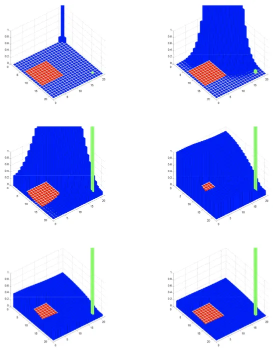
0,1 n t( ) where T represents the duration of the morphogenic event under study, and n t( ) is the number of pairs included in ItJt.In Figure 9, we represent a simulation of the perturbed diffusion process when cells and fractones exist in the ambient space. The initial distribution of growth factor is a single source (not to scale) as seen in the initial image in the upper corner above the cell, while the fractone is located near the bottom corner in green. The growth factors
32 diffuse through the free space to eventually be captured by the fractone in the last image.
33
2.3 Mitosis
As mentioned in the introduction, growth factors are regularly produced by the biological cells and then are diffusing freely in the available extra-cellular space. When the growth factor is significantly close to an active fractone, said fractone captures and concentrates the growth factor. Once the concentration of growth factor reaches a significant value, the fractone gives the order to its associated cell to undergo mitosis. In reality, the time for a cell to undergo mitosis is approximately four hours. However, by the time mitosis actually occurs, the fractone may have relocated. What is interesting is that the previous location of a fractone has been shown to be the location of new cells after the next morphogenic event. Due to this correlation, it is clear that the spatial distribution of fractones dictates the location of future morphogenic events, hence the fractones are the obvious choice to represent the controls in our system. One may argue that the reality does not match the model in that there is a time lapse in which the fractones may or may not move, and the cell undergoes mitosis. To alleviate this problem, the model is so that mitosis occurs instantaneously once an order has been issued by a fractone, and that fractone movement is also instantaneous in what we associate every available unit in Free t( )with a fractone, and that “moving" a fractone is equivalent to changing the control from 1 to 0 in one location (making this fractone inactive) and vice-versa in another location (making this fractone active). To equivalently describe this process mathematically, we state that the spatial distribution of the fractones and the concentrations of freely-diffusing growth factors dictate the location and appearance of holes (i.e. cells) in the configuration space.
Now that mitosis is occurring, a natural question arises: when a cell undergoes mitosis, how does the existing mass of cells deforms? The deformation of the mass of cells undergoing morphogenic events is extremely complex. Indeed, it involves many different criteria to take into account as well as forces to optimize. Our goal in this paper is to state and start analyzing some control problems formulated in a new setting rather than to produce the most accurate simulation of the biological process which would render such a complex system that an analytic study could not be conducted. Therefore, our criterion for the deformation of the mass of cell is based on the
34 minimization of a given distance function, based on the assumption that the mass of cell is optimizing its shape by prioritizing compactness. It is clear that we can create a slender shape, for instance, acting on the control inputs.
We assume in the sequel that we have a distance function, denoted by d, defined on the set of ordered pairs of integers. More precisely, for each a( ,a a1 2),b( ,b b1 2) , the distance between a and b is well defined by the positive real number d a b( , )
When mitosis occurs at a given time t , the configuration space Conf t( ) undergoes a topological change. Indeed, with new cells forming, they become additional holes in the ambient space, and while the dimension of Free t( ) decreases, the dimension of Cell t( )
increases. To accommodate for the formation of new cells, Cell t( ) has to deform accordingly to a prescribed algorithm. Assume unit ( , )i j represents an active fractone and we denote by C the associated cells (under our current assumptions a fractone can i
be linked up to four cells: i
14
). Since we assume all cells rigid and of equal shape, we can identify a biological cell to a single unit of our discretization.Each cell can be identified to its middle unit denoted here by ( , )a b and we can write
( , )
C a b . The deformation algorithm is defined as to preferentially deform the current mass of cells in the direction of the closest empty space in a clockwise orientation as starting from angle zero (as referenced by an axis superimposed on the center of the “mother" cell). More precisely, assume C a b( , ) duplicates. The algorithm looks incrementally for the closest unit ( , )i j Free t( )to ( , )a b (based on the chosen distance d) such that ( , )i j can be identified to a cell. Since more than one unit identified to a cell can be at the same distance from ( , )a b , we need to use a selection algorithm. There are many ways to select among those units; it could even arbitrarily be determined by the computer.
First, we need to introduce a notion of distance: let 1 ( , )a b1 1 , 2 ( ,a b2 2) , we consider the Euclidean distance:
1, 2
1 22 1 2 2E
35 As it was explained above, we assume that each cell is identified to its middle unit of its
discretization. It is therefore understood that
( , ) ( , ) ( ); 4 4, 4 4
C a b i j Cell t a i a b j b . Let Ci ( , )a bi i , i 1, 2
be two biological cells. Therefore, since between two cells we have a unit-wide channel, then a1a2mod 10 and b1b2mod 10 and d C CE( 1, 2)
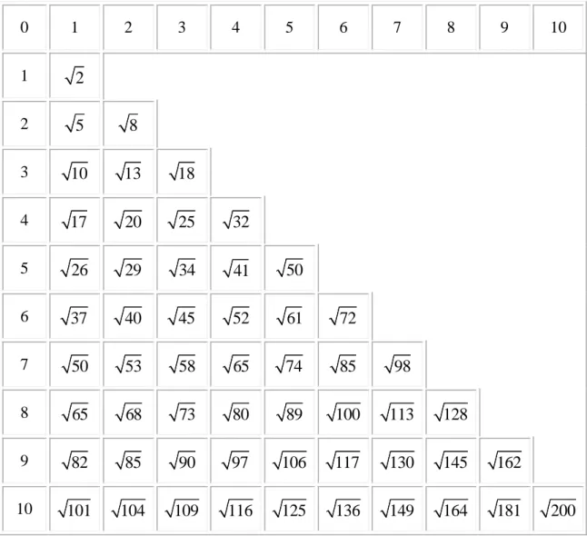
10 n2m2 | ,n m . It
follows that the deformation algorithm will search for the closest units in Free t( ) that are at distances of the form 2 210 n m from the cell undergoing mitosis. Notice that, given a cell C, the closest units multiples of 10 from C are at a distance 1 (i.e.
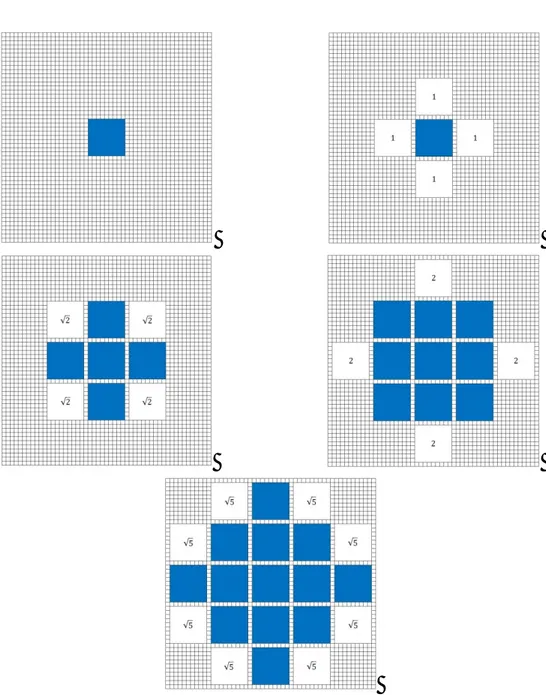
( , )n m (0,1) or (1, 0)), and there are 4 of them. The next closest units of 10 are at a distance 2 ,and there are also 4 of them. Table 2 lists some of the possible distances (divided by 10 in the table). The pattern is very clear and only one half of one quadrant is displayed since it is symmetrical with respect to the other quadrants, and the table is symmetrical about its diagonal.
As we’ll see further on, it is straightforward to relax the assumption that the distance between two connected cells is equal to 10 units or, in other words, that between two cells we have a unit-wide channel. In order to prevent confusion, we define
mod E
Dd (2.8)
36 0 1 2 3 4 5 6 7 8 9 10 1 2 2 5 8 3 10 13 18 4 17 20 25 32 5 26 29 34 41 50 6 37 40 45 52 61 72 7 50 53 58 65 74 85 98 8 65 68 73 80 89 100 113 128 9 82 85 90 97 106 117 130 145 162 10 101 104 109 116 125 136 149 164 181 200 Table 2 - D: distance distribution as measured from the "mother" cell
We have three options:
a) 12 possible units if D is an integer that is the hypotenuse of a Pythagorean triple3
b) 8 possible units if D is not along a diagonal or an axis
c) 4 possible units if D is on a diagonal or an axis, and is not the hypotenuse of a Pythagorean triple
3
A Pythagorean triple consists of three positive integers a, b, and c, such that a2 + b2 = c2. It is easy to verify from Table 2 that the Pythagorean triple (3,4,5) returns 12 units: 4 on the axis, such as (5,0) and 8 from (±3, ±4) and (±4, ±3)
37 As a resume of the notions of distance that we’ll be using, we have:
1) Distance in units: d
2) Euclidean notion of distance: d E
3) Distance between cells: D
Figure 10 - Distance distribution: an example
Now, consider for simplicity a single cell undergoing mitosis. The deformation algorithm is defined as to preferentially deform the current mass of cells in the direction
38 of empty space in a clockwise orientation as starting from angle zero (as referenced by an axis superimposed on the center of the “mother” cell). More precisely, it looks incrementally for the closest unit to ( , )i j that belongs to Free t( ). Once such a unit is detected, the deformation occurs.
Units at a same distance from ( , )i j are selected in the following order. The linear component distances, respectively, from a cell undergoing mitosis to a location toward which the mass can deform are il andi0 jl j0, for all l , where l represents the
number of possible locations at a given distance and ( ,i j represents the center of the 0 0) cell undergoing mitosis. The algorithm looks first for a unit in Free t( )such that
0 0
l
j j and chooses preferentially the max max
il . If no such unit is found, the algorithm searches for a unit in Free t( ) such that jl j0 , and chooses preferentially 0 the min
il .In the case of multiple cells undergoing mitosis, we made the assumption that there is a hierarchical rule to define which cell duplicates first: we associate to each cell an age and the oldest duplicates first (intuitively it is easy to define a scale of ages as new cells are born, and for those cells that belong to Cell t( ) |t 0 such hierarchy will be defined following the order in which the user inputs cells positions). Note that this is an arbitrary choice, that can be straightforwardly modified whenever a biological evidence dictates a more consistent rule.
Finally, if a fractone is not associate to any cell it will keep storing growth factors until a cell is close enough. At this point mitosis will occur immediately.
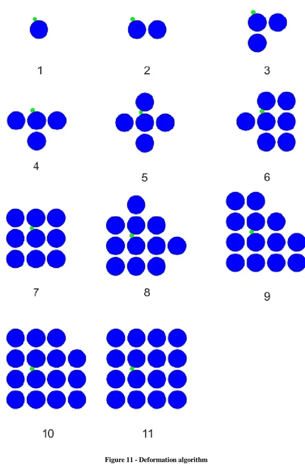
In Figure 11, we display a sequence of morphogenic events to illustrate how our deformation algorithm works. Notice that, as explained before and shown in this example, it is possible to use a discretization algorithm that associates to cells a circle inscribed in a 9 by 9 square without loss of generality. Starting from a unit cell and a single fractone that can be associated up to two cells (it is not placed at a cell corner), the sequence of images illustrate the deformation algorithm as duplication of the cell associated to the fractone occur. If we choose the origin such that the center of the initial cell is at (0, 0). we have that the initial cell space (Figure 11,1) is
39
( , )i j | 4 i 4, 4 j4
, and the final cellspace (Figure 11,11) is
( , )i j | 26 i 26, 26 j26 \
( , ) |i j i 6, 5, 5, 6,16,17 , j 6, 5, 5, 6,16,17
.Note that the ambient space is limited and gets filled up by last duplication.
When a cell undergoes mitosis and the distance algorithm has chosen a position in
( )
Free t for Cell t( ) to deform toward (let us refer to this closest selected unit at a distance D as ( , )c d ), the growth factor present in the space must move in order to make room for the deformed mass of cells. Hence, the algorithm for redistribution of GF occurs as follows:
1) it calculates the sum of the GF present in the space associated to a cell centered in unit C( , )c d where the mass of cells will deform toward, i.e.
4 , , 4 ( ) c k d l k l X t
(2.9)2) deforms Cell t( )such that ( , )c d Cell t( ).
3) counts the number of units in Free t( )Fract t( ) that are at a distance d 8 from ( , )c d .
4) distributes 70% of the sum from (1) evenly in each unit from (3).
5) counts the number of units in Free t( )Fract t( )at a distance 8d11from
( , )c d .
6) distributes the remaining 30% of the sum from (1) evenly in each unit from (5).
40 Figure 11 - Deformation algorithm
41 From the details thus far, we can glean the criteria that guide the system from one topological space to the next:
a) in the absence of cell production of GF, the initial concentration of growth factor(s) dictate how many times mitosis can possibly occur (maximum number of cells, maximum number of configurations),
b) the group of cells arrangement(s) will dictate how GF is distributed throughout, thus determining possibility for mitosis,
c) the number of fractones present will determine the maximum change in dimension at any given time t,
d) the affinity of the individual fractone to a certain GF,
e) how often the cells, now producing GFs, do this and in what amounts, f) the amount of any one GF required to initiate mitosis,
g) the “reset value” a fractone assumes post-mitosis, and h) how many cells each individual fractone is associated with.
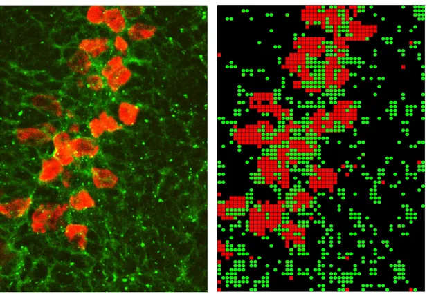
Following the mitosis algorithm defined above, we can generate a complex simulation with multiple active fractones involving several morphogenic events to reach the final desired configuration (Figure 12).
42
3. T
HEORETICAL
Q
UESTIONS AND
R
ESULTS
We can state our problem form a biological point of view:
PROBLEM -Given an initial and final configuration of cells in a prescribed ambient space, determine an initial concentration of growth factors and a dynamic spatial distribution of fractones such that the mass of cells transforms from its initial configuration to its final configuration.
Let us now rephrase this using the mathematical definitions introduced previously. To summarize, the quantity of growth factor in each unit of our discretization is regulated through the following affine control system:
0 ( , ) ( , ) ( , ) ( ) ( ) ( ) i j ( ) i j ( ), ( ) ( ) i j Diff t X t F X t F X t u t X t M t
(3.1)where the state space M t( ) dim( Diff t( )) varies with time, the vector fields F0,F( , )i j are given respectively by equations (2.3) and ((2.5),(2.6)), and such that u ( ) is an admissible control. What is unusual in the considered problem with respect to traditional control problems is that the initial and final conditions are given in terms of
(0)
Cell and Cell T( ) rather than in terms of X(0) and X T( ). More precisely, we have:
PROBLEM - Given A, Cell(0) and Cell T( ), determine X(0) and an admissible control u ( ) such that Cell(0) transforms into Cell T( ) under the evolution of system (3.1) and the prescribed rules for mitosis.
43 Notice that the admissible control is determined by the fractone set Fract t( ) at almost every time t
0,T
.The key element in our model is the role played by the fractones as controllers. Under our hypothesis, they regulate cell's proliferation and differentiation. Growth factor intervenes in cell proliferation, but the fractones are the mechanism guiding and regulating GF. In our model, the production and diffusion of GF determines the time (or equivalently the order) at which the morphogenic events take place but it is the fractones that control the process. For instance, production of GF can always be altered such that a given active fractone will reach the GF threshold at a precise time. Moreover, the results presented in this section are based on having a unique active fractone at a time. Therefore, the diffusion and production of GF does not play any role in generating the morphogenic events (it only provides temporal information). For this reason, in this chapter, we consider the simplified problem where we neglect the GF diffusion and focus on how spatial distribution of fractones regulate cell proliferation. Once again, this is not a restrictive simplification and our results can be simulated using the complete model.
The results presented in this chapter are based on the assumptions made in chapter 2, in particular we consider the algorithm for deformation of the mass of cells described above.Now that the main problem has been stated, it is clear that the algorithm we have chosen for deforming Cell t( ) (the “clockwise” arrangement starting at angle zero) is arbitrary since any two spaces are equivalent if they are rotations of a factor of 90 degrees of each other. If we had picked a different algorithm (either in direction of cell deformation or starting angle from the mother cell), the two different algorithms would produce final configurations that were a rotation of 90 n degrees from each other (for
1, 2, 3
n ).
The first two results deal with existence and uniqueness of solutions for our mathematical problem. Notice that cells are discretized as circles inscribed in a 9x9 square, without loss of generality as stated before.