3D Physics-Based Numerical Simulations of the MW6 May 29 2012 Emilia Earthquake

3D PHYSICS-BASED NUMERICAL SIMULATIONS OF THE M

6 MAY

29 2012 EMILIA EARTHQUAKE

C. SMERZINI1, I. MAZZIERI2, R. PAOLUCCI1

1

Department of Civil and Environmental Engineering - DICA, Politecnico di Milano, Milano, Italy

2

MOX-Laboratory for Modeling and Scientific Computing, Department of Mathematics, Politecnico di Milano, Milano, Italy

E-mail contact of main author: chiara.smerzini@gmail.com

Abstract. The aim of this contribution is to show 3D physics-based numerical simulations of earthquake ground motion in the Po Plain (Northern Italy) during the Mw 6.0 May 29, 2012 earthquake. The availability of a wide set of near-source records together with the knowledge on the deep structural geologic setting of the Po Plain have made this earthquake a challenging case study to verify the capabilities of physics-based simulation techniques. A spectral element model was constructed up to frequencies of about 1.5 Hz, including a 3D seismic velocity model of the Po plain, characterized by an irregular buried morphology with thickness of the plio-quaternary sediments varying from hundreds of meters to some kilometers, and an improved kinematic finite-fault rupture model, calibrated based on the available strong motion records. Numerical simulations were performed using SPEED, an open-source high-performance code, based on the Discontinuous Galerkin Spectral Elements Method (DGSEM). Overall, the comparison between strong motion records and numerical results was satisfactory, with better results for the NS component. Numerical simulations were capable of reproducing the most relevant features of ground shaking in the Po Plain during the 29 May earthquake, such as the impressive small-scale variability of near-fault ground motions, the large values of fault-normal velocity, of nearly 60 cm/s, at the up-dip stations, the generation of surface waves by the submerged topography of the Po Plain becoming predominant at long periods already at some 10 km distance from the epicenter, the spatial distribution of ground uplift with peak values of about 10 cm on the hanging wall side of the fault. Parametric analyses are also discussed to study the impact of the main modelling parameters regarding the soil behavior as well as the finite-fault rupture model.

Key Words: 3D numerical simulations, spectral elements, Po Plain earthquake, near-fault ground motions

1. Introduction

In recent years, numerical simulations of seismic wave propagation including a full 3D model of the seismic fault rupture (either kinematic or dynamic), source-to-site propagation path and complex topographic and site effects (e.g. alluvial basin) have gained an increasing attention worldwide (see e.g. [1-4]). Several numerical techniques are available, based on Finite Differences ([5, 6]), Finite Elements ([7]), and Spectral Elements ([8-10]). The most appealing features of the 3D numerical approach are: (i) modelling of the full wavefield from the extended fault rupture to the site of interest; (ii) description of the 3D variability of the dynamic visco-elastic properties of soils, having an impact on the spatial variability of ground motion; (iii) modelling of complex interaction of source effects (directivity, focal mechanism,

etc..) and localized soil irregularities; (iv) possibility to generate realistic scenarios from future earthquakes of concern for the seismic hazard at the site. On the other hand, the price for such advantages is given by the following main drawbacks: (i) frequency limitation of deterministic simulations, hardly larger than 2-3 Hz approximately; (ii) computational cost; (iii) level of detail of input geological and geotechnical data.

The main aim of this paper is to present 3D physics-based numerical simulations of the May 29 2012 Po Plain earthquake, part of an intense seismic sequence which struck a densely populated area in the Po Plain in the Emilia-Romagna region (Northern Italy) from May to June 2012. The seismic sequence was characterized by two mainshocks, the MW 6.1 May 20 earthquake at 02:03:53 UTC with epicenter at (44.89°N, 11.23°E) and 6.3 km depth, and the subsequent MW 6.0 May 29 earthquake at 07:00:03 UTC with epicenter at (44.85°N, 11.09°E) and 10.2 km depth, near the town of Mirandola ([11], http://www.bo.ingv.it/RCMT). The May 29 earthquake presents a series of interesting features, that make its study particularly challenging from a scientific point of view, i.e., (i) its dramatic impact in a densely populated urban area with a high concentration of industrial activities; (ii) the complex geological setting of a deep and large sedimentary basin such as the Po Plain; (iii) the availability of a wide near-fault strong motion dataset at deep soft sites.

Numerical simulations are performed using an innovative high-performance computer code called SPEED ([10]) based on the Discontinuous Galerkin Spectral Elements Method (DGSEM), which is particularly useful in tackling multi-scale seismic wave propagation problems in highly heterogeneous media. The application of such an approach, based on the rigorous numerical solution of the seismic wave propagation problem, including detailed 3D models both of the kinematic fault rupture and of the source-to-site propagation path, allows us, on one side, to validate the numerical model by comparison with the available earthquake recordings and, on the other side, to shed light on the most salient aspects of the seismic response at deep alluvial sites as well as of the variability of site response with respect to source-to-site propagation path, directivity effects coupled with complex local site response. After showing an overview of the seismotectocnic and geologic context, the paper presents the numerical method as well as the computational model used to simulate the May 29 Po Plain earthquake. The results of the 3D numerical simulations are, then, discussed, with reference in particular to: (i) comparison with recordings at different strong motion stations; (ii) ground shaking maps in terms of Peak Ground Velocity (PGV) and permanent ground uplift and their correlation with observed data; (iii) parametric analyses to investigate the effect of different assumptions regarding the kinematic source representation, anelastic attenuation (constant vs frequency proportional quality factor Q) and soil behavior (linear vs non-linear visco-elastic model).

2. Seismotectonic and geologic context

The 2012 Po Plain seismic sequence occurred on the southern portion of the Po Plain, a subsident EW trending foreland basin reflecting the evolution and interaction of two opposing verging fold-and-thrust belts, the Southern Alps, to the North, and the Northern Apennines foothills, to the South, which developed in response to the collision of the African and European plates from the Cretaceous onward ([12]). The Po Plain is filled with Plio-Quaternary marine and continental deposits, whose thickness ranges from a few tens of meters

on the top of buried anticlines up to about 9 kilometers in the eastern part of the basin toward the Adriatic sea. Information on the geologic setting of the Po Plain has been mostly provided by extensive hydrocarbon exploration conducted in the 1970s and 1980s ([13, 14]), hydrological studies ([15]) and by new Geological Map of Italy (1:50,000 scale,

http://sgi.isprambiente.it/geoportal). Recent works focusing on the collection and elaboration of such information can be found in [16] and [17]. The structural map of Italy is reproduced in FIG. 1.

Three main arcs of blind, N-verging thrusts and folds compose the outermost sector of the Northern Apennines, corresponding to the Po Plain, namely, from west to east: Monferrato, Emilia and Ferrara-Romagna. The 2012 Emilia seismic sequence reactivated the central section of the Ferrara-Romagna arc around the town of Mirandola (see surface projection of the causative fault in FIG. 1). The seismic sequence was recorded by different accelerometer networks operating on the Italian territory (see e.g. [18, 19]). It is worth underlining that 34 stations recorded the earthquake within an epicentral distance Re < 30 km, providing a wide and high quality near-fault strong motion dataset (see filled dots in FIG. 1).

FIG. 1 Structural map of Italy, reproduced from [14], where the different shades of green denote the depth of the base of Pliocene; the epicenter (star) along with the surface projection of the fault of the

29 May earthquake and the available strong motion stations (filled dots) are also indicated.

3. The numerical code: SPEED

The open-source software package SPEED (SPectral Element in Elastodynamics with Discontinuous Galerkin: http://speed.mox.polimi.it/), developed in the framework of a joint research program between the re-insurance company Munich RE and Politecnico di Milano, is designed for the simulation of large-scale seismic wave propagation problems including the coupled effects of a seismic fault rupture, the propagation path through Earth’s layers, localized geological irregularities, such as alluvial basins, and soil-structure interaction problems (see e.g. [10]). Based on a discontinuous version of the classical spectral element (SE) method, as explained in [20], SPEED is naturally oriented to solve multi-scale numerical

problems, allowing one to use non-conforming meshes (h-adaptivity) and different polynomial approximation degrees (N-adaptivity) in the numerical model. SPEED is designed for multi-core computers or large clusters (e.g., Fermi BlueGene/Q at CINECA), taking advantage of the hybrid MPI-OpenMP parallel programming.

The present version of SPEED includes the following features: i) different seismic excitation modes, including kinematic finite-fault seismic ruptures models; ii) both linear and non-linear visco-elastic soil materials; iii) different attenuation models with frequency proportional quality factor ([21]) or frequency constant quality factor following the Generalized Maxwell body model (GMB) (see [22, 23]); (iv) paraxial absorbing boundary conditions ([24]); (v) time integration by either the second order accurate explicit leap-frog scheme or the fourth order accurate explicit Runge-Kutta scheme.

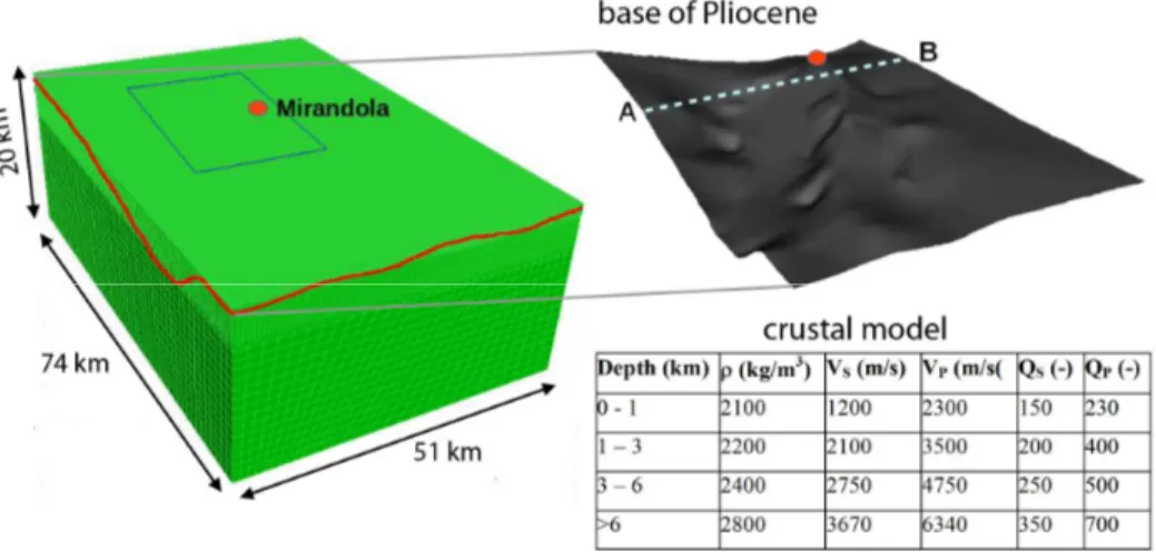
4. Computational model

The computational model adopted for the numerical simulation of the MW 6.0 May 29 earthquake extends over a volume of about 74x51x20 km3 and includes the following distinctive features (see FIG. 2):

- kinematic representation for the seismic fault rupture of the 29 May earthquake; - inclusion of a 3D velocity model of the Po Plain, taking into account the spatial

variation of the most relevant geologic discontinuities beneath the surface sediments, and a horizontally layered crustal model (see table in FIG. 2);

- flat free surface due to the small topographic variations of the investigated area;

- linear visco-elastic behavior with frequency proportional Q factor (Q0 is defined at the reference frequency f0 = 0.67 Hz);

Details about the aforementioned aspects are given in the following. Different modeling assumptions regarding the soil behavior will be addressed in Section 7.

FIG. 2: 3D mesh model of the May 29 Po Plain earthquake with indication of the shape of the base of Pliocene formations (see shades of green in FIG. 1).

4.1 Kinematic fault model

Starting from a seismic source inversion study based on observed coseismic deformations ([25]), the kinematic slip model has been improved by considering the large number of available near-source strong motion records to obtain a satisfactory fit between synthetics and observations. Further details on the calibration of the slip model can be found in [26]. The resulting slip distribution together with the kinematic source parameters (fault geometry, location of hypocenter, scalar seismic moment, rise time, source time function) are shown in TABLE 1. The source model is characterized by rather shallow asperities with maximum displacement of about 70 cm, lying at about 6 km depth, which, coupled with the depth of the hypocenter location, favor up-dip directivity effects that may explain the large velocity pulses observed in the Mirandola area.

4.2 3D velocity model

The 3D seismic velocity model adopted in the simulations is summarized in TABLE 2. Two main geologic interfaces were considered: first, the base of Quaternary sediments (zQ) was estimated from the geological cross-sections available within the study area combined with the quantitative evaluation of sediment thickness at several selected stations to provide the best fit on near-source record; second, the base of Pliocene formations (zP) was derived from the structural map of Italy (see shaded tones in FIG. 1, top panel). Modelling the variability of the Quaternary sediments thickness throughout a small spatial range around Mirandola, was found to play a key role to simulate with reasonable accuracy the prominent trains of surface waves observed along the Mirandola structural high.

4.3 Mesh

The numerical model is discretized using an unstructured conforming hexahedral mesh with characteristic element size ranging from 150 m at the surface to about 1500 m at the bottom of the model, see FIG. 2. The mesh can propagate frequencies up to about 1.5 Hz using a third order polynomial approximation degree. Hence, the model consists of 1’975’240 spectral elements, resulting in approximately 150106

degrees of freedom. The time integration has been carried out with the leap-frog scheme, choosing a time step equal to 0.001 s for a total observation time T = 30 s.

The simulations have been carried both on the IDRA cluster located at MOX - Department of Mathematics, Politecnico di Milano, Italy (http://hpc.mox.polimi.it/hardware/) and on the FERMI cluster located at CINECA, Bologna, Italy (http://www.hpc.cineca.it/). As indicator of the parallel performance of the code SPEED, we report herein that the total simulation time (walltime) for a single run on Fermi using 4096 cores was about 5 hours.

TABLE 1: Kinematic fault parameters. Fault Origin (FO) refers to the uppermost fault vertex at zero strike.

Fault parameter Value for 3D modelling

M0 9.35 10

17

Hypocenter (°N, °E, Depth) (44.851, 11.086, 10.4)

L / W (km) 22 / 12

Fault Origin FO (°N, °E) (44.900, 10.914)

Top depth (km) 3.7

Strike / Dip / Rake (°) 95 / 60 / 90

Rise Time  (s) 0.7

Rupture Vel. VR (km/s) 0.85VS Slip time function s(t)

 

TABLE 2: 3D velocity model. zQ and zP denote the base of Quaternay and Pliocene, respectively.

Geologic Unit Depth z (m)  (kg/m3) VS (m/s) VP (m/s) QS (-) Quaternary z ≤ 150 1800 300 1500 30 150 < z ≤ zQ 1800 + 6(z-150)0.5 300 + 10 (z-150)0.5 1500 + 10 (z-150)0.5 VS/10 Pliocene zQ < z ≤ zP 2100 + 4 (z-zQ) 0.5 _{800 + 15 (z- z} Q) 0.5 _{2000 + 15 (z- z} Q) 0. VS/10 Before

Pliocene z > zP See crustal model (FIG. 2)

5. Comparison with strong motion observations

FIG. 3 shows the comparison between synthetics and observations in terms of three-component velocity waveforms at six representative SM stations (see location in FIG. 1). Both recorded and simulated waveforms were band-passed filtered with an acausal 3rd order Butterworth filter between 0.1 and 1.5 Hz, the latter being the frequency resolution of the numerical model. On the whole, the agreement between synthetics and records is good in both time and frequency domain, especially on the horizontal NS and vertical component for almost all considered stations. In particular, the agreement of the large NS velocity pulse, with filtered PGV of around 50 cm/s, at the closest stations to the epicenter (i.e., MRN and MIR01) is remarkable and points out the relevant role of up-dip directivity effects on ground motions.

The agreement for the EW component is not as satisfactory as for the NS component, especially at those stations located at short epicentral distance, approximately less than 5 km, while the comparison improves at larger distances. This is probably due to the insufficient complexity both of the seismic fault and of the geological models, being nearly symmetric in the epicentral area with respect to the NS direction. A more detailed description of the performance of the simulations, measured through quantitative goodness of fit criteria, can be found in [26].

In FIG. 4 the comparison between observations and synthetics is reported also for a roughly NS array of temporary stations (MIR array as sketched on the right panel of the figure) in terms of velocity waveforms only for the NS component. It is found that numerical simulations can predict with reasonably accuracy the onset of a train of northwards propagating surface waves, generated by the buried morphological irregularity of the Mirandola structural high. This is a peculiar feature of the Po Plain earthquake: a complex superposition of body and surface waves in the near-source region, the latter becoming predominant already at some 10 km, as highlighted by the long period components in the coda of the signals.

FIG. 3: Comparison between recorded (black line) and simulated (red line) three-component velocity time histories (0.1-1.5 Hz) at six representative strong motions stations.

FIG. 4: Comparison between recorded (black line) and simulated (red line) NS velocity waveforms (0.1-1.5 Hz) along the MIR array.

6. Spatial variability of near-fault ground motion

FIG. 5 (left) illustrates the spatial distribution of PGV (gmh, geometric mean of horizontal components), as predicted by our physics-based 3D numerical simulations. For comparison, the observed gmh values of PGV, obtained at the available SM stations in the same frequency range of 3D numerical simulations, are depicted by filled dots. The comparison with the available SM data points out that numerical simulations reproduce with good accuracy the peak ground motion amplitudes (around 60 cm/s at Mirandola) as well as the spatial distribution of seismic shaking in the epicentral area. Although not shown here for sake of brevity, the two-lobed pattern of the PGV map turns out to be fairly consistent with the spatial distribution of macroseismic intensity, IMCS (see [27]).

As a further check of the accuracy of the numerical simulations, we show in FIG. 6 the comparison between the map of permanent ground displacement, as computed by SPEED (left), with the geodetic observations (right) made available from the Synthetic Aperture Radar (SAR) Interferometry survey COSMO-SkyMed ([11]). The geodetic measures provide a value of maximum ground uplift on the hangingwall of the fault of about 10 cm, which is substantial agreement with the synthetic estimates (computed as the average of the unfiltered vertical displacements over the last 5 s of the signal), except for a slight under-prediction of uplift on the Western side of the fault area.

FIG. 5: PGV (gmh, geometric mean of horizontal component) map from 3D numerical simulations with indication of the observed values at the strong motion stations (filled dots). Adapted from [26].

FIG. 6: Map of permanent ground uplift simulated by SPEED (left) and observed by COSMO-Skymed InSAR processing (right), from [26].

7. Parametric analyses

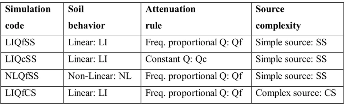
To analyze the impact of the main modelling parameters regarding the soil behavior as well as the finite-fault rupture model, parametric simulations were carried out by varying the hypothesis concerning: i) the soil behavior: linear (referred to hereafter as LI) vs non-linear (NL); ii) anelastic attenuation features: frequency proportional vs constant quality factor Q (Qf vs Qc, respectively); iii) the degree of complexity of the kinematic source model characterized by either constant – “simple” source (SS) - or stochastic kinematic parameters – i.e. “complex” source (CS). Specifically, in addition to the reference simulation presented in the previous

sections, namely, LIQfSS (linear visco-elastic + frequency proportional Q + simple source), three further simulations were performed, as summarized in TABLE 3.

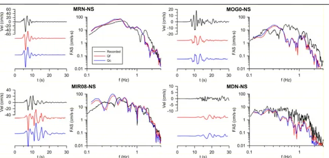
The assumed parameters are summarized in the following sub-sections, which will focus on the comparison of the parametric analyses with respect to the reference simulation. For sake of brevity, attention will be limited to four strong motion stations located at short to intermediate epicentral distances, namely, MRN (Re = 4.1 km), MIR08 (Re= 7.3 km), MOG0 (Re= 16.4 km) and MDN (Re= 27.5 km), and to one ground motion component, i.e., NS component, which is the most critical for this earthquake.

7.1 Effect of quality factor

For the simulations with constant Q (Qc), the Generalized Maxwell Body (GMB) model was assumed with the following parameters: n = 3, min = 20.1 rad/s (note that max = 100  min), and we fix QP() = VP/10 and QS() = VS/10 for the soils inside the alluvial basin (for the values in crustal layers see table in FIG. 2).

FIG. 7 shows the comparison between simulations LIQfSS and LIQcSS. Note that assumption of frequency proportional Q implies that all frequencies are equally attenuated, while a constant (hysteretic) Q leads higher frequencies to be attenuated more with an exponential trend. Given the short distances involved, less than 30 km, and also the maximum frequency of the simulation, equal to 1.5 Hz, the effect of quality factor turns out to be rather limited. However, the effect of Q starts being tangible at distant stations, such as MDN, where, the amplitudes of higher harmonics (f > 0.6 Hz) are more attenuated under the hypothesis of constant Q.

TABLE 3: Summary of parametric analyses.

Simulation code Soil behavior Attenuation rule Source complexity

LIQfSS Linear: LI Freq. proportional Q: Qf Simple source: SS

LIQcSS Linear: LI Constant Q: Qc Simple source: SS

NLQfSS Non-Linear: NL Freq. proportional Q: Qf Simple source: SS LIQfCS Linear: LI Freq. proportional Q: Qf Complex source: CS

FIG. 7: LIQfSS vs LIQcSS: comparison of velocity time histories and corresponding Fourier amplitude spectra for the NS component at four representative stations (MRN, MIR08, MOG0,

MDN).

7.2 Effect of non-linear visco-elastic soil behavior

For the non-linear simulations, the G/G0- and damping- curves, as derived by [28], were used for the top 150 m layers, see FIG. 8.

In FIG. 9 the comparison between LIQfSS and NLQfSS is presented for the same component (NS) and set of representative stations as considered previously. Overall the effect of non-linearities is not very significant. The effect of non-linear behavior is more pronounced at those stations located at very short distances (Re < 8 km), i.e. MRN and MIR08, where peak ground motion values reach significant values, up to about 55 cm/s. At these stations, the lengthening of period due to non-linear effects in the soft alluvial deposits can be found in the low period range (< 1 Hz). In the high period range, say between 1 and 1.5 Hz, a counterintuitive effect is noted in particular at MRN station: amplitudes for the NL cases are larger than the ones for the LI case, probably due to additional spatial heterogeneity features introduced by the non-linear assumption.

FIG. 8: G/G0- and damping- curves adopted for the non-linear simulations (from [28]).

FIG. 9: LIQfSS vs NLQfSS: same as in FIG. 7.

7.3 Effect of stochastic source parameters

Following the procedure described in [29], random perturbations of kinematic fault parameters, such as rise time, rupture velocity and rake angle, satisfying the Von Karman spatial correlation model with along-strike and down-dip correlation lengths equal to around 3 km, were assigned. The parameters are listed in TABLE 4.

FIG. 10 illustrates the effect of a “complex” source model (LIQfCS) with respect to the “ simple” one (LIQfSS) with constant average parameters across the fault plane, under the hypothesis of frequency proportional Q and linear behavior. It is noted that the effect of the random source parametrization is to increase moderately the amplitude of frequencies above around 0.5 Hz. At MOG0 such an effect is less obvious probably due to the limited influence of the source details and up-dip directivity conditions, as this station is located along the fault strike direction (other stations are oriented as the fault normal approximately) near the western border of the fault trace.

TABLE 4: Parameters for the correlated random fault rupture model.

Source parameter Average Value Max variation w.r.t. mean Correlation

coefficient with slip

Rise time 0.7 0.50 0.50

Rupture Velocity 0.85VS 0.30 0.30

FIG. 10: LIQfSS vs LIQfCS: same as in FIG. 7.

8. Conclusions

Stimulated by the availability of a wide set of strong motion records as well as of detailed knowledge of the subsurface soil model, this work has focused on the generation of 3D physics-based numerical simulations of the May 29 2012 Po Plain earthquake.

Numerical simulations were carried out through SPEED, a discontinuous Galerkin spectral element code. Comparison between synthetics and observations was satisfactory at the majority of strong motion stations, especially on the NS component (which is the one that recorded the largest amplitude of almost 60 cm/s), while less convincing results were obtained for the EW component probably owing to insufficient complexity both of the seismic fault and of the geological model. Some important evidence of the observed earthquake ground motion was accurately reproduced, such as, at very short epicentral distances (< 5 km), the large fault normal velocity peaks at the up-dip stations and the remarkable small-scale variability, and, at larger distances (already at some 10 km), the predominance of northwards propagating surface waves, the map of ground uplift on the hanging wall side of the fault, and the two-lobed pattern of the horizontal PGV map.

Furthermore, the parametric analyses illustrated in the paper have shown that the modelling assumptions regarding the soil behavior (attenuation rules and linear vs non-linear behavior) and the complexity of the source may have an impact on the simulated ground motions, depending on the source-to-site distance and level of excitation.

The May 29 2012 earthquake was a challenging case study to validate and explore the capabilities of the existing physics-based numerical approaches to predict the variability in space and time of the most relevant strong ground motion features, based on a full 3D model of the seismic source process, the propagation path and localized geologic features. Such simulations are, in fact, expected to become, in near future, the most promising tool for the prediction of earthquake ground shaking scenarios, in alternative to standard approaches based on Ground Motion Prediction Equations, especially for the following aims: i) better constrained seismic hazard assessment in those magnitude and distance ranges which are

poorly constrained by recorded data, i.e., typically in the near field and for large magnitude earthquakes (MW>7.0-7.5); ii) for seismic hazard and risk analyses of large urban areas, where preserving the full spatial correlation of ground motion may be crucial, and of critical structures, such as nuclear power plants, for which a detailed simulation of the physics of the earthquake may have a great impact on the reduction of uncertainty (sigma); iii) deeper understanding of the variability of earthquake ground motion and of its spatial correlation features resulting from the complex combination of the fault rupture process and wave propagation effects.

Acknowledgements

This work was partly funded by ENEL, Italy, under contract n. 1400054350, in the framework of the international SIGMA Project, by the Italian Department of Civil Protection, within the DPC-RELUIS (2014-15) RS2 Project, and by MunichRe, Germany. The CINECA award under the LISA and ISCRA projects is also gratefully acknowledged, for the availability of high performance computing resources and support.

REFERENCES

[1] JONES, L.M., et al., “The ShakeOut scenario”, Technical Report USGS-R1150, U.S. Geological Survey and California Geological Survey (2008)

[2] GRAVES, R.W., et al., “CyberShake: a physics-based seismic hazard model for Southern California”, Pure and Applied Geophysics 168 (2010) 367–381.

[3] PAOLUCCI, R., et al., “Physics-based earthquake ground shaking in large urban areas”, in Perspectives on European Earthquake Engineering and Seismology, Second European Conference on Earthquake Engineering and Seismology, Istanbul, 24-29 August (2014) [4] BILEAK, J., et al., “The ShakeOut earthquake scenario: Verification of three simulation

sets”, Geophysical Journal International 180 (2010) 375–404.

[5] GRAVES, R. W. “Simulating seismic wave propagation in 3D elastic media using staggered-grid finite differences”, Bull. Seismol. Soc. Am. 86 (1996) 1091–1106

[6] PITARKA, A., “3D elastic finite-difference modeling of seismic motion using staggered grids with nonuniform spacing”, Bull. Seismol. Soc. Am. 89 (1999) 54–68

[7] BIELAK, J., et al. “Parallel octree-based finite element method for large-scale earthquake ground motion simulation”, Computer Modeling in Engineering and Science

10 (2005) 99–112.

[8] FACCIOLI, E., et al., “2D and 3D elastic wave propagation by a pseudo-spectral domain decomposition method”, J. Seismol. 1 (1997) 237–251

[9] KOMATITSCH, D., VILOTTE, J.-P. “The spectral-element method: An efficient tool to simulate the seismic response of 2D and 3D geological structures”, Bull. Seismol. Soc. Am. 88 (1998) 368–392.

[10] MAZZIERI, I, et al., “SPEED: SPectral Elements in Elastodynamics with Discontinuous Galerkin: a non-conforming approach for 3D multi-scale problems”, International Journal of Numerical Methods in Engineering 9 (2013) 991--1010.

[11] PEZZO, G., et al., “Coseismic deformation and source modeling of the May 2012 Emilia (Northern Italy) earthquakes”, Seism. Res. Lett. 84 (2013) 645–655.

[12] BURRATO, P., et al., “Is blind faulting truly invisible? Tectonic-controlled drainage evolution in the epicentral area of the May 2012, Emilia-Romagna earthquake sequence (Northern Italy)”, Annals of Geophysics 55 (2012)

[13] PIERI, M., GROPPI, G., “Subsurface geological structure of the Po Plain, Italy”, CNR, Progetto Finalizzato Geodinamica, 414 (1981) 1–13.

[14] BIGI, G., et al., “Structural model of Italy 1:500,000”, CNR Progetto Finalizzato Geodinamica (1992)

[15] RER (Regione Emilia Romagna, Servizio Geologico Sismico e dei Suoli) & ENI-AGIP “ Riserve idriche sotterranee della Regione Emilia-Romagna”, Di Dio (Ed.), S.EL.CA., Florence (1998)

[16] FANTONI, R., FRANCIOSI, R., “Tectono-sedimentary setting of the Po Plain and Adriatic foreland”, Rend. Fis. Acc. Lincei 21 (2010) S197S209.

[17] MOLINARI, I., et al., “Development and testing of a 3D seismic velocity model of the Po Plain sedimentary basin, Italy”, Bull. Seismol. Soc. Am. 105 (2015) 753–764

[18] LUZI, L., et al., “Overview on the strong-motion data recorded during the May–June 2012 Emilia seismic sequence”, Seism. Res. Lett. 84 (2013) 629–644.

[19] CASTRO, R. R., et al., “The 2012 May 20 and 29, Emilia earthquakes (Northern Italy) and the main aftershocks: S-wave attenuation, acceleration source functions and site effects”, Geophysical Journal International 195 (2013) 597–611.

[20] ANTONIETTI, P. F., et al., “Non-conforming high order approximations of the elastodynamics equation”, Comput. Meth. Appl. Mech. Eng. 209-212 (2012), 212 – 238 [21] STUPAZZINI, M., et al., “Near-fault earthquake ground-motion simulation in the

Grenoble valley by a high-performance spectral element code”, Bull. Seismol. Soc. Am.

99 (2009) 286–301.

[22] EMMERICK, H., KORN, M., “Incorporation of attenuation into time-domain computations of seismic wave fields”, Geophysics 52 (1987) 1252-1264.

[23] MOZCO, P., et al. “The Finite-Difference modelling of earthquake motions: waves and ruptures”, Cambridge University Press (2014)

[24] STACEY, R., “Improved transparent boundary formulations for the elastic-wave equation”, Bull. Seismol. Soc. Am. 78 (1988) 2089–2097.

[25] ATZORI, S., Personal Communication (2012).

[26] PAOLUCCI, R., et al., “Anatomy of strong ground motion: near-source records and 3D physics-based numerical simulations of the Mw 6.0 May 29 2012 Po Plain earthquake, Italy”, Geophysical Journal International, in press (2015)

[27] GALLI, P., et al., “Rilievo Macrosismico MCS speditivo, Terremoti dell’Emilia - Maggio 2012”, Tech. rep., Dipartimento della Protezione Civile, Final Report (2012) [28] FIORAVANTE, V., GIRETTI, D. “Amplificazione sismica locale e prove dinamiche in

centrifuga” (in Italian), Parma (2012).

[29] SMERZINI, C., VILLANI, M. “Broadband numerical simulations in complex near field geological configurations: the case of the MW 6.3 2009 L'Aquila earthquake”, Bull. Seismol. Soc. Am. 102 (2012) 2436–2451.