Department of Economics and Statistics
Doctoral Thesis in Economics Cycle XXXIII
Coordinator Prof. Michelangelo Vasta
Three Essays on the measurement of
socioeconomic inequalities and well-being
Scientific-disciplinary sector: SECS-P/01
PhD student: Giovanna Scarchilli
Supervisor: Prof. Paolo Brunori
Academic Year: 2020-2021
lmente da SCARC HILLI GIOVA NNA C=ITDr. Giovanna Scarchilli
Submitted to the Department of Political Economy and Statistics, University of Siena, in partial fulfilment of the requirements for the degree of Doctor of Philosophy in Economics.
Abstract
The complex transmission mechanism of socioeconomic inequalities takes place in several spheres of life. This Doctoral Thesis, composed of three essays, focuses on the characterisation of some components of inequalities and their spread through social groups. In the three contributions, innovative techniques have been exposed and em-pirically assessed to extend the literature on the measurement of well-being and the study of social inequalities. The first essay represents a study on teenagers’ leisure time activities distribution and how it relates with income and subjective well-being realisations. Taken from the German Socioeconomic Panel (SOEP), the information on leisure time activities has been processed with a network-based technique to build a multidimensional index proxying well-being. The second essay presents an evolutionary analysis of cumulative deprivation for the Italian working-age population between 2007 and 2018. A rank-based multidimensional approach is applied for the identification of the cumulatively deprived people. Therefore, an assessment of the statistical multidi-mensional dependence lying across the identified deprivations is provided following a copula-based technique. The third essay contains a focus on the transmission of health inequality through the socioeconomic background of people. A machine-learning tech-nique is used to derive the population partitioning into social groups and to define the different opportunity backgrounds. Furthermore, the study provides insights re-garding the varying effect of individual health-related behaviours on the health status. The 2011 sample of UK Household Longitudinal Study data is used for the empirical application.
Keywords: socioeconomic inequalities, multidimensional indicators, economic com-plexity, copula function, inequality of opportunity.
List of Figures iv
List of Tables vi
List of Abbreviations viii
1 Introduction 1
2 Measuring the complexity of leisure time: a new methodological pro-posal to study how the use of leisure time relates with well-being 7
2.1 Introduction . . . 7
2.2 Methodology . . . 11
2.2.1 Concluding remarks on the methodology . . . 15
2.3 Data . . . 17
2.4 Empirical application . . . 20
2.5 Conclusions . . . 27
2.6 Theoretical Appendix . . . 29
2.6.1 Random Walk definition . . . 29
2.6.2 Algebraic interpretation of the Method of Reflections . . . 29
2.6.3 Nestedness test . . . 31
Bibliography . . . 32
3 The evolution of cumulative deprivation: a multidimensional copula-based approach 34 3.1 Introduction . . . 34
3.2 Methodological framework . . . 39
3.2.1 Copula Function . . . 39
3.2.2 The measures of dependence and the copula sections . . . 42
3.3 Data . . . 47
3.4 Results and discussion . . . 50
3.5 Conclusions . . . 63
3.6 Theoretical Appendix . . . 66
3.6.1 The positional outcomes are the margins of the cumulative dis-tribution function FX . . . 66
3.6.2 The probability Integral Transform Theorem . . . 66 iii
4 Model-based Recursive Partitioning to estimate Unfair Health
In-equalities 70
4.1 Introduction . . . 70
4.2 Inequality of Opportunity: from theory to practice . . . 75
4.2.1 Model frameworks . . . 75
4.2.2 Estimation methods and IOP measurement . . . 80
4.2.3 Criticism around the traditional empirical applications . . . 83
4.2.4 A new generation of empirical applications: a detailed illustration 84 4.3 Estimation Strategy . . . 90 4.4 Data . . . 92 4.5 Estimation Results . . . 95 4.6 Conclusions . . . 101 Bibliography . . . 103 Appendices 106
A Data and Tables 106
B Data and Tables 110
2.1 The Individual-Activity network, an example . . . 10
2.2 Network of individuals and activities sorted by their Complexity . . . . 16
2.3 Complexity VS Ubiquity - 2006 . . . 21
2.4 Complexity VS Ubiquity - 2011 . . . 22
2.5 Complexity VS Ubiquity - 2016 . . . 23
2.6 Interpreting of Individual Complexity as Human Flourishing . . . 24
2.7 Average complexity by parental support - Top 20 VS bottom 80 complex people. . . 27
3.1 Independence Copula (two dimensions) . . . 41
3.2 Fréchet-Hoeffding Bounds (F-H) . . . 42
3.3 Contour plot of the Independence copula . . . 44
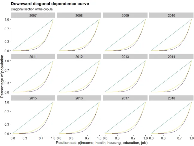
3.4 Downward Diagonal Dependence Curve . . . 45
3.5 Cumulative deprivation from a time series perspective . . . 52
3.6 Cumulative deprivation from a time series perspective . . . 53
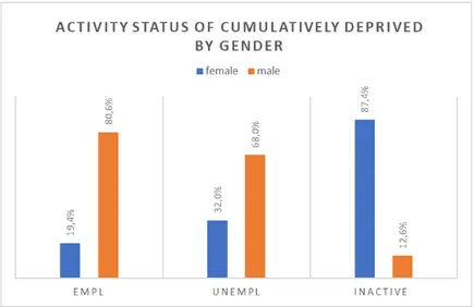
3.7 Cumulatively deprived males and females by activity status . . . 54
3.8 Yearly downward diagonal dependence curves . . . 56
3.9 Downward diagonal dependence indices: comparing the full 5-dimensional set with 4-dimensional sets . . . 58
3.10 Percentage of cumulatively deprived who are counted in the AROPE index 60 3.11 Comparison between cumulative deprivation incidence (left-axis) and other socioeconomic indicators: AROPE rate (right-axis) and Absolute poverty incidence (left-axis). . . 61
3.12 Poverty thresholds comparisons . . . 62
3.13 Poverty thresholds comparisons . . . 63
3.14 Poverty thresholds comparisons . . . 63
3.15 Poverty thresholds comparisons . . . 64
4.1 Type-specific income distributions . . . 77
4.2 Relation between allostatic load and effort . . . 96
4.3 Model-based partitioning: Health to effort relation by circumstances. . 98
4.4 Health-to-effort relation by type . . . 99
4.5 Type specific effort densities. . . 100
A.1 Summarising the average individual complexity by levels of life satisfac-tion - Size of each level group . . . 109
2.1 Spearman Correlations table . . . 24
2.2 Average Complexity by life satisfaction level - 2011 . . . 25
2.3 Average Complexity by household income decile - 2011 . . . 26
3.1 Comparing two hypothetical societal multidimensional distributions . . 36
3.3 Description and methods of construction of the selected well-being di-mensions . . . 49
3.4 Presence of cumulative deprivation among three most frequent cases . . 51
3.5 Population in Cumulative Deprivation by Socio-Demographic Charac-teristics . . . 54
3.6 Partial dominance comparisons . . . 57
4.1 Summary statistics: Allostatic load (H) and Effort (E) . . . 92
4.2 Correlation between effort and lifestyle variables . . . 93
4.3 Descriptive statistics - Circumstances . . . 94
4.4 Regression coefficients for each terminal node (population type) . . . . 97
4.5 Within type descriptive statistics . . . 98
4.6 Average health outcome by type and effort quantile . . . 100
4.7 Direct Unfairness for each specific effort quantile - Bootstrapped results 101 4.8 Fairness Gap for each specific reference type - Bootstrapped results . . 101
A.1 Summary statistics - Year 2006 . . . 106
A.2 Summary statistics - Year 2011 . . . 107
A.3 Summary statistics - Year 2016 . . . 107
A.4 Mean Difference Test . . . 108
A.5 Mean difference between the two samples . . . 108
B.1 Average diagonal dependence indices comparisons . . . 111
B.2 Total population: Cumulative deprivation, gender and activity status . 113 C.1 Missing values among circumstance variables, net of the item missingness present on purpose . . . 114
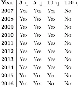
A-F Alkire and Foster, (2011)
AROPE At Risk of Poverty and Social Exclusion ARP At Risk of Poverty
DDI Diagonal Depenendence Index DU Direct Unfariness
EU-SILC European Union Survey on Income and Living Conditions F-H Fréchet-Hoeffding Bounds
F&S Fleurbaey and Schokkaert, (2009) FG Fairness Gap
FMM Finite Mixture Models ICI Individual Complexity Index IOP Inequality of Opportunity LCA Latent-Class Analysis LWI Low Work Intensity
MOB Model-Based recursive Partitioning MoR Method of Reflections
PCA Principal Component Analysis RCA Revealed Comparative Advantage SAH Self-Assessed general Health
SOEP German Socio-Economic Panel
Introduction
Perhaps stimulated by the disillusionment that the financial and economic crisis of 2008 has put forward, within the last decade the topics of poverty and well-being have gained increasing attention both in the academic world and in the public debate. On the policy side, we have witnessed at many examples of institutional and governmental initiatives to observe and monitor the social and economic conditions of people. In the EU, among the most famous relevant policy stimuli can be found the European Union’s 2020 growth strategy (2010), and the Sarkozy Commission on the Measurement of Economic Performance and Social Progress (2008), led by J-P Fitoussi and the former Nobel prizes J. Stiglitz and A. Sen.
In the following years, the OECD’s project on Measuring the Progress of Soci-eties (2013), the European Pillar of Social Rights - with a constant update of ‘social scoreboards’ officially entering the European Semester of economic policy coordination since 2017 -, and the UN’s Agenda 2030 for Sustainable Development (SDGs, 2013) have been some of the outcomes of the aforementioned contributions.
Despite the initial enthusiasm which characterised the period of programming poli-cies for realising and implementing the European targets, the ten-year-after analysis on the fulfilment of the EU2020 strategy came across with some delusion. Furthermore, the recent COVID-19 pandemic has newly exacerbated old vulnerabilities, wiping out years of economic recovery and social progress. A sign of this significant impact has been the recent rise of the inactive and unemployed population as being primarily composed of self-employed, young, females, and temporary-contract owners. On top of that, we are witnessing at the surge of new forms of weaknesses. For example, the lockdown caused an abrupt increase in the school dropout incidence across the coun-tries’ most economically poor areas. This phenomenon will strongly contribute to the increase of inequalities due to different opportunities.
Given the situation illustrated above, the academic and non-academic stakehold-ers have always had a keen interest in studying, on the one side, the phenomenon of socioeconomic inequalities, and, on the other, the related policies and their outcomes. The academic attention towards the studies of socioeconomic inequalities can be traced back to the seminal contribution of A. Sen (1980; 1987). Sen stressed on the necessity of studying societies going beyond the sole income measure and considering societal welfare in a broader sense. In so doing, he gave a notable contribution to the spreading of studies related to well-being. These studies led the researches to employ multidi-mensional approaches to be able to tackle them. Beside the theoretical component, the increased coverage of life dimensions in survey data and the growing number of com-putational techniques to aggregate and process the data-collected information gave a valuable contribution to this subject matter.
From a political and philosophical point of view, there is no unique and all-encompassing definition of the concept of ‘well-being’. Nevertheless, there is general agreement that well-being is the outcome of a complex system of interrelationships between the so-cial and economic sphere, including subjective and objective aspects. It is precisely the word multidimensional that represents a common thread across the three essays displayed in this thesis.
From an analytical perspective, social scientists have dealt with the measurement of well-being using a variety of statistical tools and models - each and every variety is motivated by given assumptions. The underlying assumptions of the models are both related to prescriptive or normative decisions of the researcher, and to the various necessary decisions related with the empirical application. Despite the clear distinction between the definition of the two types of assumptions, there can be some overlap in the implications of both, when applied. As a result, it is noticeable that among applied researchers in socioeconomic inequalities and well-being two subgroups have emerged: on the one hand, those who favour purely normative assumptions, whilst on the other, those who rely on data-driven techniques to make a decision on certain assumptions. The differences emerge on several stages of the studies on well-being, poverty, and inequalities measurements - among them, the definitions of poverty and well-being, the construction of relevant population groups which are the target of a policy, the setting and validation of relevant parameters for the empirical analysis.
This PhD thesis belongs to that "group" that employs data-driven techniques. However, it does not actually reject to make normative considerations on the phenom-ena under study. Indeed, it is believed that data-driven methods does not represent a perfect substitute to the normative choice of a policy maker. While the data-driven
methods are able to provide clear information on what is happening in the society, normative positions state what should be happening in the society. Therefore, the for-mer could be seen as a support to address traditional normative issues, which did not find a universal ethical agreement. Moreover, the most relevant innovation brought by data-driven methods is the capacity to recognise new matters and find new solutions, which could be unexpected when approaching those studies that take normative deci-sions. Furthermore, data-driven methods could be very useful to solve some relevant practical issues related to traditional empirical approaches, which are acknowledged to be determining serious biases in the results.
Combining ideas from economic theory, philosophy, sociology, and data science this thesis provides innovative tools to interpret socioeconomic inequalities and measure well-being. Despite their "distance" regarding the means used in each empirical appli-cation, the essays together attempt to provide a set of tools to enrich with practical computational examples specific parts of the literature on well-being and inequalities. The recurring innovative element of the thesis is precisely the exploration and adapta-tion of new multidimensional measurement techniques. Furthermore, each contribuadapta-tion attempts to contextualise the novelties within the well-being and inequalities’ litera-ture domain. However, it should be emphasised that such approaches all refer to the individual sphere, and therefore they do not take into account trends in inequalities related to different observation units, e.g. households and territorial.
This dissertation consists of three essays, each of them is presenting an innovative technique to study well-being measurement, which supported by an illustrative empir-ical application of the new approaches’ advances and limitations. The chapters follow the structure of academic papers. Each essay is self-contained and can be read inde-pendently.
In the first essay, in Chapter 2, a network-based approach is used to build a mul-tidimensional index of well-being for teenagers. The well-being status of people is proxied by processing information about several leisure activities. This study aims to assess how the information on the use of time, if observed at youth, can add valuable information on future well-being realisation.
The specific multidimensional index technique employed for this experiment is the "Economic Complexity Index" of Hausmann and Hidalgo (2014). This technique uses the information provided by the network which maps the links between two entities, namely individuals and everyday life activities, in order to provide a ranking of the sample considered. The everyday activities are different in terms of the required effort and cost to be sustained. For this reason, there is high variability in the distribution
of people’s time employment.
Behind the adoption of the "Economic Complexity Index", which provides a rank-ing of people accordrank-ing to their use of time, is that, not only specialisation matters, but also diversity is the key to measure human complexity. Firstly, the choices and capabilities of individuals are identified through the observation of the "specialisation" of people in a specific activity, i.e., whether such activity is considerably present in the overall activity set of a person. Second, each activity is defined by its “sophistication”. Third, the eclecticism of individuals in terms of the multiplicity of their activities and interests, is considered. The data used for computing the Complexity index comes from the special module dedicated to 17 years old respondents of the German Socio-economic Panel (SOEP), which contains information on their weekly activities. An attempt to use the complexity index as a predictor of subjective and material well-being as recorded in later waves of the survey is proposed, despite the strong sample attrition. From the exercise it emerged that a high complexity for individuals is associ-ated with social activities. Very ubiquitous activities, such as watching TV, are instead associated with low-ranked people in the complexity score. Very specialised activities, e.g., playing an instrument, are instead quite rare and associated with mid-complex people. The complexity ranking are correlated with current subjective well-being per-ception, and with the economic conditions of the individual in the future.
As stressed within the literature on poverty and social exclusion, there are many forms of deprivation which tend to come together in societies. The evolution of cumu-lative deprivation is addressed in Chapter 3, regarding the working-age population in Italy between 2007 and 2018. Cumulative deprivation is characterised by disposable income, health status, housing quality, job conditions and educational attainment. All the dimension-related outcomes are observed at the individual level in each single year using the cross-sectional EU-SILC data.
In this paper, a copula-based technique is adopted to estimate the dependence lying among the multiple dimensions of cumulative deprivation. Copulas are used in statistics to evaluate the degree of dependence within a rank-based multidimensional framework; therefore, they have been gaining attention in social studies for inspecting the properties of interrelations taking place among different unit variables. A very recent contribution by Decancq (2020) offers a toolkit to address the analysis of the dependence at the extremes of the distributions’ multiple dimensions of well-being: the diagonal dependence index.
In the period considered, the cumulatively deprived population in Italy shows a growing trend, amounting approximately to one million individuals in 2018. A
visi-ble peak of the phenomenon, with respect to the total sample, emerges in 2014 and 2015, highlighting a visible correlation with the trend of the estimated dependence index for the empirical multidimensional copula. The presented index of multidimen-sional dependence could be interpreted as measuring the degree of association between the various forms of deprivations taken into consideration. Given its proximity to the concept of poverty, cumulative deprivation has been contextualised with respect to the current estimates of relative and absolute poverty provided by the Italian Na-tional Statistical Institute (ISTAT). A descriptive comparison is provided between the maximum income of cumulatively deprived people by household type and geographic location, with two poverty income thresholds (the AROPE and the ISTAT’s Absolute poverty estimated thresholds).
The last essay, in Chapter 4, provides a zoom on a narrower well-being aspect, the individual health. The COVID-19 pandemic’s disruption has put under the spotlight the highly unequal distribution of health characterising current societies. Furthermore, health deprivation has shown strong links with deprivation of other facets of life. In-dividual health is hereby conceived as an objective status of well-being summarising a series of biomedical characteristics of the person. The health inequality is studied from a multidimensional perspective, more precisely, referring to the theory of Inequality of Opportunity in order to assess its relation with other socioeconomic inequalities. The socioeconomic drivers of inequality of opportunity (IOP) in health are investigated and some light is shed on the methodological progress that characterises the IOP models. IOP in health is assessed controlling also social group-specific trends of health-related behaviours in the determination of the health outcome. Despite the health-related behaviour is considered as a proxy of effort, its connection with the social background is kept into consideration within the model framework. The application introduces a new methodology – the Model-Based Recursive Partitioning (MOB) – to derive the population groups while estimating, within each group, the relation between the health status and the effort variable. This study represents an empirical application of the measure of the “direct unfairness” and the “fairness gap”, as proposed by Fleurbaey and Shokkaert (2009).
The empirical application is conducted using the UK Household Longitudinal Panel Survey. This dataset, in wave 2, contains data nurse-recorded on a sub-sample of the whole database regarding physical biomarkers. This information has been aggregated into a general index defining the physiological health condition of each individual. The evidence coming out by the adoption of the MOB technique shows a significant role of the socioeconomic background of people in determining health outcomes. Furthermore,
it emerges clearly that, the behaviours are significantly affecting the health status with a different magnitude according to the social group of belonging. Despite the lower return to efforts that we observe among the most disadvantaged social groups, the distribution of behaviours show a slightly higher average effort for those with poorer socioeconomic background.
Measuring the complexity of leisure
time: a new methodological proposal
to study how the use of leisure time
relates with well-being
2.1
Introduction
"The quality of life depends on people’s objective conditions and capabili-ties." Stiglitz et al. (2009)1
Although per capita income is still, by far, the most popular measure of well-being, there have been various proposals to extend the horizon of its measurement. Inspired by the works of Fleurbaey et al. (2008); Stiglitz et al. (2009), many scholars have studied well-being from a multidimensional perspective, involving both material and subjective aspects of life. Overall, well-being can be either measured as a multidi-mensional composite indicator through the aggregation of multiple items (Costanza et al., 2016; Deutsch and Silber, 2005; Peña-López et al., 2008; VanderWeele, 2017), or as a single-domain measure such as material, or subjective well-being (Diener, 2009; Kahneman and Krueger, 2006).
While studying individual well-being - both material and subjective - a growing attention has been paid to the observation of the use of time. In their detailed study on the use of time across countries, Esteban Ortiz-Ospina and Roser (2020), for the project
1This statement is one of the twelve recommendations of the Report of the Commission on the
Measurement of Economic Performance and Social Progress written by Stiglitz et al. (2009)
"Our World in Data", stated: "Studying how people spend their time represent an important perspective for understanding living conditions, socioeconomic opportunities, and general well-being".
Regarding the literature on well-being and time use, on the one side, there are stud-ies focusing on analysing social inequalitstud-ies and the allocation of leisure time activitstud-ies (Aguiar and Hurst, 2007; Burchardt, 2008; Lippe et al., 2010; Merz and Rathjen, 2014). On the other side, scientific production is widening following the work of Kahneman and Krueger (2006), which proposed to combine the use of time with affective ratings to analyse a societal well-being score and a rank the activities observed. In both cases, the time use is valuable information for proxying well-being. The latter studies aim at giving more consistency to the notion of subjective well-being and life satisfaction, while assuming the intrinsic value of an activity that can be defined by the emotions reported by the individual. The former studies keep the analysis perspective on a less personal level and they analyse how the use of time relates not only with subjective well-being but also with other notions of well-being.
With this study, the information on the distribution of leisure time use across the population is analysed to produce an index that could rank activities and individuals invoking the various notions of life-satisfaction and material well-being, by gathering them into a broader concept of human flourishing (VanderWeele, 2017).2 The study
presented introduces a data-driven methodology to collect and process information on leisure time use data, and to rank activities performed in the leisure time and individuals observed in a certain period of their life.
The aim of this paper is that to introduce a way to study a specific social group ac-cording to the use of leisure time observed, and furthermore, that to contextualise such information in the broader box of well-being notions. The main underlying assumption of this methodology is that the distribution of the use of time across individuals and leisure activities create a complex network of capabilities and opportunities, which can evaluate both the single activity and the individual with respect to the others. In the context of activity-related capabilities, specialisation is a plus. However, specialisa-tion is not enough to observe multifaceted abilities or social integraspecialisa-tion. In order to observe whether ones’ abilities are valuable and enrich the individual well-being, it is possible to refer to the diversity of specialisations and the ubiquity of the activities. These two "ingredients" characterise the so-called individual complexity and the activ-ity complexactiv-ity. The information extrapolated through the complexity rankings is used to proxy the means and capabilities acquired by the person and necessary to study
2VanderWeele (2017) defines human flourishing as a multi-domain concept involving the
future realisations of material well-being and life satisfaction.
With this paper, individual complexity is defined and its relation with well-being is explored. The considered leisure time activities provide a wide range of information due to their quantitative and qualitative heterogeneity. The subjects of the empirical application correspond to the sole group of teenagers. The decision to focus on a specific age group is that the variability of activities and leisure time use strongly depend on the age distribution. Moreover, the choice of this specific cohort represents a way to proxy individual capabilities formation and both relate them with current socioeconomic conditions and with future well-being realisations.3
As already anticipated, the main innovation of the study is the adoption of a new technique for processing information on the time use distribution. “Borrowed” from the macroeconomic literature on trade and growth, the adopted measure is the Economic Complexity Index. The Economic Complexity represents a measure of the capability of a country to be the major exporter of a diverse series of goods which are rare and highly required, and it has been successfully translated in the added value of knowledge accrued by a country through development and economic growth. This widely notorious measure, in the specific purpose of this study, is given the name of Individual Complexity Index, when referred to the people, and Activity Complexity Index, when referred to the activities observed.
This indicator – which is hereby believed to have a good potential within the use of cross-sectional micro-economic data – aggregates the data making use of the Method of Reflections (MoR), an algorithm presented by Hausmann and Hidalgo (2014) for creating their Economic Complexity Index. The main information necessary for the implementation of the new Individual Complexity Index is provided by the network which maps the links between two entities: the individual and the activities he makes in his free time. The algorithm’s inputs are the diversity of the people’s activity sets and the ubiquity of every single activity across the population. The MoR is a recursive algorithm that repeatedly corrects one measure with the other to enlighten the in-depth information on each person and activity, which does not emerge at first sight.
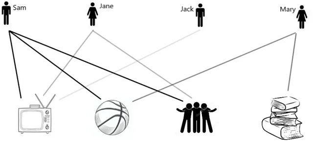
Figure 2.1 is a graphical representation of the concepts of diversity and ubiquity through a very simple example of individual-activity network.
As it is possible to see from the figure, Sam watches TV, plays basketball and spends time with friends. Therefore, one could say that he has a diversity score of 3, whilst Jane and Mary have a diversity of 2 and Jack only of 1. There are in total three people watching TV, thus this activity has a ubiquity score of 3. Despite Mary and
3This conceptualisation takes inspiration to the work of Sen (1993) only in the form of the
Figure 2.1: The Individual-Activity network, an example
Jane have the same diversity, Jane is doing an activity that is very ubiquitous, whereas Mary reads a lot of books, which is quite rare.
The algorithm of Hausmann and Hidalgo (2014) captures all this information in an iterative way and produces a complexity ranking of all the people and the activities.
With this application, it is possible to observe a wide set of leisure activities carried out by a population of 16/17-years-old individuals: the data used for the computation come in fact from a special model built on respondents aged 16/17 of the German Socio-Economic Panel (SOEP). The network linking people and individuals is computed the observation of the activity-specific distribution of time use across people. The link between a person and the activity is indicating that the person devotes a considerably high amount of time to that activity with respect to the rest of the people. The aim of this application is the exploitation and the exploration of the informative power of Individual Complexity and the evaluation of its capacity to proxy individual well-being in various forms.
The complexity index is assumed to be useful to describe the well-being of people. More specifically, a positive relation is expected between complexity and well-being in various forms. The impact of material household well-being is assumed to be positive as well on the current complexity.
Therefore, the analysis is run over two binaries. On one side, the complexity out-come is contextualised with respect to the leisure time activities observed and with the current subjective and material well-being of the teenager. On the other side, an
analysis on the interrelation between individual complexity and future realisations of well-being is provided. The analysis presented does not investigate causation rules but simply correlation patterns.
The empirical application represents an initial exploration of the possible adapta-tion of this technique to a different context. From a technical perspective, the use of the MoR’s aggregation technique contextualised within multidimensional well-being, enables to contribute to the literature on composite indicators regarding data-driven weighting procedures.4 Within the family of data-driven methods, the frequency
tech-niques are widely used among multidimensional poverty indices. Given the association of the frequency of (no-)deprivation concept with the ubiquity and diversity, the pre-sented complexity index could be placed within the data-driven weights classification, in particular linking it to the frequency techniques.
The paper is structured in the following sections. Section 2.2, contains an illustra-tion of the methodological background of the Economic Complexity Index. In Secillustra-tion 2.3 follows a description of the data used for the empirical application. In Section 2.4, the empirical results and interpretations are provided. The last Section reports a conclusive discussion on the empirical application.
2.2
Methodology
The MoR computation’s first step is the construction of the individual-activity network, which is created by following a relative frequency rule. The (bipartite) individual-activity network can be associated with a binary bi-adjacency matrix M. The links of the bipartite network are determined by an index transformation of the original quantity of unit time that an individual spends averagely on the specified activity.
The applied transformation represents a weighting procedure of the importance of the activity in terms of, i) the whole activity set of the specified individual, ii) the total amount of the activities considered, which, afterwards is converted into a binary matrix. This transformation can provide a measure of Revealed Comparative Advantage, which is hereby interpreted as a measure of Revealed Comparative Affection (Revealed Comparative Advantage (RCA)) of an individual regarding a certain activity. The so-called RCA, or "Balassa Index", has been adopted by Hausmann and Hidalgo to generate the binary bi-adjacency matrix necessary to implement the algorithm for the complexity computation, the Method of Reflections.
The rationale behind the RCA computation is to derive the value of the match
4See Decancq and Lugo (2013) for an extensive discussion on the role of weights in
between all individuals and the activities basing on the person’s revealed comparative affection towards each activity. The matches define a bipartite network that filters the links between the individual and the activity, keeping only the individual affections. By means of this, the concept of well-being which can be extrapolated is adapted to this exercise of grasping the differences across peoples’ opportunities, stimuli and interests, and, consequently, at ranking them.
The input for the RCA computation is the original data matrix containing the time spent per activity, P
n×m, where i = 1, ..., n and a = 1, ..., m respectively the number of
the individuals and of the activities. The value for each match between individual i and activity a in the RCAi,a results from the following operation:
RCAi,a =
si,a
ta
(2.1) where the value si,a represent the time spent by individual i on activity a with
respect to the total time spent on leisure activities by individual i. This value is collected in a matrix S obtainable by dividing the total time each person spend in the activities considered P
a
pi,a to the original P matrix. This matrix represents a
scaling factor for the time-unit spent by the individual i in each activity as a ratio of total (a = 1, ..., m) activities done. The value ta represents the sum of all the time
each individual has devoted to a specific activity a, its corresponding collection for all activities is the vector T .
S n×m= Pn×m/ X a xi,a, Ta 1×m =X i S n×m (2.2)
Dividing Si,a by the element Ta, a further scaling of the individual amount of time
per activity is provided with respect to the other people. The RCA matrix from Eq.2.1 illustrates, for every individual, the revealed comparative affection towards each activ-ity. In other words, the RCA shows which individual is devoting a "greater than usual" portion of time in a certain activity.
When RCAi,a > 1, it means that an individual i does an activity a for a portion of
time that is greater than the average amount of time dedicated to such activity by other people. Furthermore, such activity is a considerable part of the overall ith individual
activity set. Defining the bi-adjacency matrix as M, the value of the match in the case of an RCAi,a> 1, is mi,a = 1. Alternatively, the value of the match is mi,a = 0, if the
portion of activity done by an individual is very small compared to its activity set and the total amount of consumption of this good, (RCAi,a ≤ 1). Therefore, single value
of the bi-adjacency matrix, mi,a, is used to build the individual-activities bipartite network as follows: Mi,a= 1 if RCAi,a > 1 0 if RCAi,a ≤ 1 (2.3) The M matrix has size (n × m).From now on, any reference to the activity per person coincide with the match as shown in Eq.2.3 in which the individual shows a greater than 1 revealed comparative affection towards a specific activity.
The RCA represents the first step of the weighting scheme between dimensions of leisure time. At this stage, the weight is converted into a binary variable dividing the population in two groups, namely the individuals who keep the dimension as essential and those who do not. This procedure attaches “same weight” equal to 1 to all the dimensions with a high RCA score. Otherwise, it equals to 0. All the activities are considered as perfect substitutes and they are measured with the same unit, i.e. time. Thus, the activities are observed through a frequency approach.
Afterwards, the information retained is the degree of the nodes within the individual-to-activity network Mi,a. The node degrees in this bipartite network are respectively
the measures of diversity and ubiquity: ki,0 and kg,0. The node degree of individual1 is
equal to the sum of all the edges that start from a particular vertex, the individual1,
connecting another vertex.
The diversity measure of a specific individual is the sum of all the activities done by an individual:
ki,0 =
X
a
Mi,a (2.4)
While the ubiquity measure of a specific activity is the sum of all the individuals who consume it:
ka,0=
X
i
Mi,a (2.5)
The diversity vector ki,0 n×1
, and the ubiquity vector ka,0 1×m
, contain respectively the mea-sure computed for each individual and good.
The Index of Individual Complexity, can be obtained by the standardisation of the resulting vector ki,N where the subscript represents the Nth iteration of the Method
of Reflections for the individual i. Symmetrically, the Activity Complexity can be obtained by the standardisation of the resulting vector ka,N. 5
com-The Method of Reflections is an iterative algorithm combining the information provided by the individual-activity network properties. Each iteration computes a value representing an approximation of the conditional probability to move through the network’s links to reach a specific individual starting from a different one. Before explaining its implicit meaning, it is worth to present its algebraic construction.
The MoR performs N iterations simultaneously for the individuals and the activi-ties. The first iteration brings respectively to the average ubiquity of the activities done by individual i (Eq.2.6) and the average diversity associated to activity a (Eq.2.7):
ki,1 = 1 ki,0 X a Mi,aka,1 (2.6) ka,1= 1 ka,0 X i Mi,aki,1 (2.7)
Therefore, by recursively plugging the output in Eq.2.6 in the successive iteration of Eq. 2.7, up to the Nth time, it is possible to obtain the following results:
ki,N = 1 ki,0 X a Mi,aka,N −1 (2.8) ka,N = 1 ka,0 X h Mi,aki,N −1 (2.9)
Plugging the recursion at (N − 1) of Eq.2.9 in the recursion at N of Eq.2.8, it is possible to obtain a formula that expresses the diversity recursion as a function of the initial conditions and the diversity of the other individuals (i0) who perform the same
activities of i. ki,N = X i0 ˜ Mii0ki0,N −2 (2.10)
The new system obtained contains a matrix called ˜Mii0.
˜ Mii0 = X a Mi,aMi0,a ki,0ka,0 (2.11) The Eq.2.10 represents the individual-activity network as a Random Walk process and ˜Mii0 is the transition matrix. Eq.2.11 expresses the probability of reaching
indi-vidual i, starting from indiindi-vidual i0 and passing through the activities they carry out.
plexity (Hausmann and Hidalgo, 2014). For what concerns the activity complexity the Nthiteration approaches an odd number around 19.
The bigger is the similarity of two individuals’ activity set, the higher will be their proximity in the final ranking obtained by the Complexity Index.6
We can say that at the Nth iteration, k
i,N is a linear combination of the elements
of the initial step ki,0 where the coefficients result by the product of all the degree of
nodes lying in the path, which connect the individual i0 to individual i (Hidalgo and
Hausmann, 2009).
With a higher number of iterations, it is possible to grasp more information from both characteristics. Therefore, the correlation between the initial and the final itera-tions is decreasing in the number of iteraitera-tions.
Given that the sequence ki,s converges to a vector with all equal values for s → ∞,
the difference between subsequent elements in the sequence of ki,N and its limiting value
progressively shrinks (wi = ki− ki,N). According to the algebraic interpretation of the
matrix ˜M, the iterative process let the result of Eq.2.10 to converge to the eigenvector of the matrix in Eq.2.11 associated with the second highest eigenvalue of the matrix
˜ M.7
Given that we are working with a bipartite network, the even and odd iterations have different meanings. More precisely, there is a clear interpretative distinction between these two variables (Caldarelli et al., 2012). For what concerns individuals, the even variables (ki,0, ki,2, ...) are generalised measures of diversification of their activity
sets, while the odd variables (ki,1, ki,3, ...), are generalised measures of the ubiquity of
the activities. Furthermore, the two sequences ki,N and ka,N are inversely related. This
means that people who are highly diversified in terms of activities done, will more likely being doing also activities which are rare (less ubiquitous), while very common activities will tend to be associated with less diversified people.
2.2.1
Concluding remarks on the methodology
The RCA index can extract the information concerning the individual level of affection towards a specific activity defined through a relativistic approach. This index collects only information regarding the time-use unit measures, but it attaches a constant sub-stitutability measure to all the activities considered. The value judgements regarding each activity depend only on their distribution across the population, and the frequen-cies observed imply a certain data-driven outcome on the network.
6Section 2.6 illustrates the definition of a Random Walk process in the network theory framework. 7(Kemp-Benedict, 2014). An extensive discussion on this statement is presented in the Theoretical
Recalling the inverse relationship between diversity and ubiquity, and contextualis-ing it in the macroeconomic context, it is possible to find the emergence of a contrast between the traditional Ricardian theory of specialisation and the message brought by the Method of Reflections. While Ricardo predicted that specialisation in a narrow sector is the ”virtuous” path for growth of a country, the Economic Complexity conveys a different message. The rationale behind MoR and Economic Complexity is that, not only specialisation matters, but also diversity is a pathway to growth.
Therefore, as far as high complexity is associated with high diversity, low ubiquity will be as well related with high complexity. In order to provide a graphical intuition of this relation, Caldarelli et al. (2012) suggest to represent the individual-activity network - the binary matrix P - having sorted all the people and all the activities by increasing complexity. More precisely, the activities - the columns of the matrix - are sorted in ascending complexity from the left to the right. The people - the rows of the matrix - are sorted in ascending complexity from the bottom to the top.
Fig.2.2 shows the bi-adjacency matrix of the bipartite network of people and activ-ities in 2011, both elements are sorted by increasing Complexity Index scores.8
Figure 2.2: Network of individuals and activities sorted by their Complexity
It is worth reminding that the network shows the links between the people and the activities assigned with the RCA index. The dark red spots identify those individuals dedicating a higher quantity of time with respect to the average time spent by other people to a specific activity (RCA index = 1). The more red spots are appearing
alongside a row, the more diversified is the individual activity set. Likewise, the more red spots are appearing alongside a column the more frequently is the single activity appearing across various activity sets. On the contrary, the orange spots show a non-significant consumption amount (RCA index = 0).
People at the bottom of the y-axis of figure 2.2, are associated with the lowest complexity. The higher the complexity of the activities, the more on the right corner a given activity will appear.
If complexity preserves the relation with diversity and ubiquity as explained above, the resulting matrix should look like a triangular matrix. If we would have observed a higher polarisation towards specialisation, this matrix would have looked like a block diagonal matrix, whilst, instead, it is more likely to be an upper triangular matrix. In order to algebraically test whether the diversity and ubiquity contribute to define a complex system, Caldarelli et al. (2012) propose to test the nested structure of the matrix of the bipartite network.9 In graphical terms, a nested bi-adjacency matrix
shows that the number of the links in each row, from the lower to the upper one, is a subset of the previous row.
Being the individual-activity network a nested structure, some characteristics con-cerning both the activities and the individuals observed are implied. First, a randomly chosen activity appearing in a highly diversified individual’s activity set will likely be a non-ubiquitous activity. By contrast, a randomly chosen activity that appears in poorly diversified activity sets will less likely be complex good. Second, a randomly chosen individual who does very frequently a highly ubiquitous activity is not likely to be highly diversified. Conversely, a randomly chosen individual that does most of the time a rare activity is more likely to be highly diversified. The system’s nestedness is also a necessary condition of well-behaviour of the algorithm of the MoR adopted to obtain the Complexity Index.
2.3
Data
The empirical application has been realised using data on the use of time from the Youth Questionnaire of the SOEP. The SOEP is a wide-ranging representative lon-gitudinal study of private households. The computation is provided on a constant activity set for population samples referred to different years 2006, 2011 and 2016. The dataset containing the leisure activities questionnaire is referred to young respon-dents aged 16 or 17. Furthermore, the same individuals who took part to the 2011
9The nestedness is a statistical property of bipartite networks when are represented as a triangular
youth questionnaire sample have been sampled from the individual adult dataset of 2016. The following list exposes the SOEP data sets were necessary for the empirical application. The list indicates the number of observed individuals net of the missing values on the leisure activities and on the sample attrition.
• wjugend: Individual questionnaire for people aged 16-17, year 2006 (N = 286) • bbjugend: Individual questionnaire for people aged 16-17, year 2011 (N = 506) • bgjugend: Individual questionnaire for people aged 16-17, year 2016 (N = 493) • bbh: Household questionnaire, year 2011 (N = 506)
• bbp: Individual questionnaire, year 2016 (N = 188)
The reasons that led to the employment of the youth questionnaire are mainly three. Firstly, there is a trade-off between the specificity of the activities observed and the variety of the individuals’ characteristics. For example, the average disposable leisure time for an adult with a family is lower than the one of a teenager. Given that the person-to-activity network is obtained with a frequency approach, the age is a source of heterogeneity for which it is necessary to control. The ideal application would be a computation of the complexity ranking for each specific age class. Furthermore, an age specific computation allows for varying the activity set considered. Secondly, the choice of the data on the teenagers allows to measure the value of leisure time when there is no - or at least lower -, trade-off between it and the income earnings. Lastly, a possible connection with the Equality of Opportunity theory could be done if consid-ering the value of Individual Complexity as an outcome variable whose determinants beyond individual control are represented by the current household economic status. On the contrary, the Individual Complexity is considered to be a determinant of fu-ture realisations of material well-being status and both current and fufu-ture subjective well-being status.
The activities for which the time frequencies are observed are watching television, surfing on the internet, listening to music, playing an instrument or singing, doing sport, dancing or acting, doing tech-activities (coding and programming), reading, spending time with girl/boyfriend, best friends, clique, going to a youth centre, volunteering activity, going to religious initiatives, relaxing (or none of the other alternatives).10
The complexity algorithm adopts a relativistic perspective which strictly depends on the distributions observed at time t. Thus, there could be some dependence of
the outcome on the activities distribution characteristics regarding each point in time. The empirical computation is performed for three different years in order to control, at least partly, for the relativistic perspective inherent to the results. The data which have been employed exploit the panel structure of the SOEP - following the same individual throughout time -, and through the observation of different samples in different years. Each activity is associated with a score, which defines the frequency of use of a person. The frequencies have been normalised on a monthly scale, as shown in the following table:
Survey time definition Frequency per month
Daily 1
Weekly 10/30
Monthly 4/30
Rarely 1/30
Never 0
The Complexity Index is the result of a recursive bipartite iteration, hence, both the individual and the activities are ranked – in this regard, it is interesting also to observe an activity-specific pattern in the ranking process-.
Therefore, in order to extrapolate some useful insights regarding the activity rank-ing, the activities have been divided into two groups, whether they are considered as social or non-social activities.
On data attrition
The merge between the 2011 teenager dataset with the individual adult data of 2016 presents the 62% of attrition. Hence from the 506 individuals in the original sample the population observed five years later is composed of 188 individuals (the 37%). Among those people who do not appear in the individual questionnaire five years later, the 53% are people who, having changed their place of residence with respect to the household included in the panel, vanish form the questionnaire. The remaining 47% of missing matches appear only in the households questionnaire. There has been a drastic reduction of the representative power of the outcoming dataset. Therefore, there might be strong biases emerging from the analysis due to the plausible correlation between social and economic conditions of those who could afford leaving parental home before 23 and those who could not. It is plausible that parents support the longer education of their children with a longer cohabitation. This could mean that the people who remain
in the panel are mostly people who decided to continue their studies with tertiary education. By contrary, who left the parental home between 18 and 23 might be who economically emancipated through work or who, with the financial support of their parents could leave the parental home for continuing the education elsewhere. Given that most of the general socio-demographic information is not available in the youth questionnaire (the gender is missing as well), it is not easy to identify specific attributes who correlate with the disappearance from the panel, neither to assess which portion of them are missing at random. Therefore, the entity of the attrition could be verified through the mean difference analysis between the attributes observable within the two samples. As it emerges from the table A.4 in the Appendix A, the complexity ranking on the sub-sample of people observed five years later does not show a statistically significant mean with respect to the total sample. Moreover, table A.5, shows that there is no significant change in the means of each activity between the two samples. Hence, although the Complexity index’s descriptive parameters are not demonstrated to be significantly varying across the samples, the level of attrition brings with it obvious problems in the ability to generalise what emerges from the time analysis.
2.4
Empirical application
Economic growth models traditionally conceive the specialisation as a strength. The primary reference may be the Ricardian model of specialisation. The experiment of Hausmann and Hidalgo (2014) shows however, that this prediction is not correct: the “diversity” factor also plays a central role in the development of a country. Although this study’s subject switches from the country to the individual, the same principle stands for the latter unit of observation. The higher is the diversity and the complexity of people, the better we would expect to be their well-being status.
By contrast, the more a specific activity is spread out across the population, the less complex will be the individuals who mostly spend their time on it. As a result, there is an inverse relationship between the complexity of activities and their ubiquity scores.
The illustration of the complexity outcome is presented initially from the point of view of the activities, afterwards, from the point of view of the individuals. This is due to the fact that understanding how complexity relates with certain activities helps to understand as well the individual complexity measure as a function of the leisure time activities.
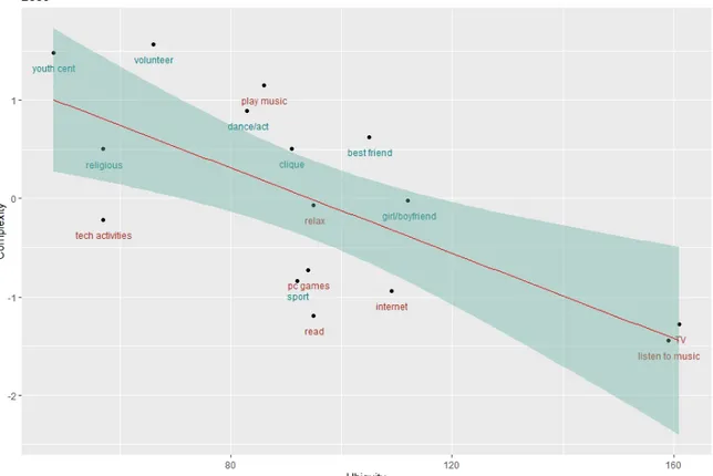
A complete picture regarding the activities’ complexity could be provided by the observation of the relation between complexity and ubiquity. Therefore, figures 2.3,
2.4 and 2.5 depict the relation identifying the activities’ characteristics for the three years considered. It is possible to consider these figures as able to provide a sort of ”identikit” of the complex activities and to evaluate whether it emerges a stable rela-tionship between the observed activities and their complexity ranking across time.
Figure 2.3: Complexity VS Ubiquity - 2006
Figures 2.3, 2.4 and 2.5 show the relation between the complex activities and their ubiquity score. As expected, there is an inverse relationship between the complexity of an activity and its ubiquity. From a year-by-year perspective, it emerges that, despite not all the single observations fall in the confidence interval, the rankings assigned to the different activities in terms of complexity and ubiquity of activities is somehow stable.
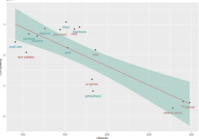
Dividing the activities into two groups according to whether these are social or individual activities, it emerges that social activities are mostly associated with higher complexity. This relation results visibly stable across years. The ”social” activities are those including people of similar age spending time with each other. In the plots, it is possible to distinguish the social from the non-social activities by the colour of the labels. In all the three years, a higher concentration of social activities is evident
Figure 2.4: Complexity VS Ubiquity - 2011
in the graph’s top-left corner, where the complexity score is high. The worst ranked activities are stable across the years: spending time watching TV, listening to music and, for 2016, being on the social networks. These activities are widespread across a population of 17-years-old individuals and, for this reason, they clearly end up being the less complex.
Which is a plausible interpretation of the Individual Complexity ranking? In which way is such ranking related to a human flourishing notion? How can be the top-ranked complex people described? We discuss the answer providing some outstanding results. As seen from the previous figures, there is a pattern which emerges spontaneously across each yearly complexity VS Ubiquity plot, the distribution of social activities. Indeed, it emerges that social activities are non ubiquitous and always associated with high complexity.
The relationship between the scores of the individual complexity and the intensity of social activities is a notable support of the intuition concerning the role of social activities.
Figure 2.5: Complexity VS Ubiquity - 2016
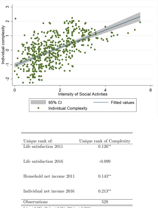
Figure 2.6, shows the fitted relation between the individual complexity and the intensity of social activities appearing in the time use set of people.
Based on the amount of social activities every person declared to be doing on a weekly or daily basis, figure 2.6 shows a dispersion plot throughout complexity scores. From the plot emerges a strictly positive relation between the two series, a further element in the support of the interpretation which links individual complexity with human flourishing.
In which way is Human Flourishing - intended as a fertile network of social connec-tion and active social participaconnec-tion - positively linked to both subjective and objective dimensions of well-being?
Although it has been already depicted how any evolutionary analysis may not be fully reliable due to the panel data attrition as illustrated in Section 2.3, it will follow a discussion on how the complexity index correlates with contemporary and future realisations of income and life-satisfaction. Table 2.1 illustrates the Spearman rank correlations between the Individual Complexity and both current and future material and subjective well-being.
Figure 2.6: Interpreting of Individual Complexity as Human Flourishing
Unique rank of: Unique rank of Complexity
Life satisfaction 2011 0.126∗∗
Life satisfaction 2016 -0.099
Household net income 2011 0.143∗∗
Individual net income 2016 0.213∗∗
Observations 529
∗ (p < 0.05),∗∗ (p < 0.01),∗∗∗ (p < 0.001)
As it emerges from table 2.1, there are significant rank correlations between the complexity and the material conditions observed in 2011 and 2016, and between the complexity and the contemporary individual satisfaction. Future subjective life-satisfaction appears to be uncorrelated with the ranking of past complexity, yet it turns out to be negatively related with complexity. This is somehow not surprising given the strong role of temporary feelings involved in the subjective well-being measures, which make it hardly comparable across time.
Despite the analysis presented does not provide a basis for a causation relation, the association of complexity with contemporary and future well-being metrics is intended to justify two distinct empirical studies. On one side, a more accurate definition of teenager complexity may result from the role of contemporary household characteristics and well-being. On the other side, individual complexity could be studied form the perspective of a future well-being determinant.
The contemporary relation between complexity, life-satisfaction and household in-come is further explored in the next tables. Tables 2.2 and 2.3 respectively provide a purely descriptive relation between the average complexity and by levels of life satis-faction and by income deciles.
More accurately, tables 2.2 and 2.3 show the average individual complexity levels in 2011 for life-satisfaction levels and current household income deciles.
Individual Complexity Life satisfaction (mean) (sd) (N)
1 -1.288 . 1 3 0.222 1.051 10 4 -.5385 1.027 14 5 0.0446 0.890 30 6 -0.147 0.957 36 7 -0.064 1.001 80 8 -0.0589 1.013 166 9 0.104 0.978 125 10 0.316 1.021 43 Total 0.002 0.998 505
Table 2.2: Average Complexity by life satisfaction level - 2011
A visible increase in the average complexity in the population observed emerges in the group of higher-income deciles and the higher life-satisfaction levels. How-ever, especially by focusing on life-satisfaction, it is noticeable that some groups are dramatically small, therefore they lack of valuable generalising power over the whole
Individual Complexity Income deciles (mean) (sd) (N)
1 -0.309 0.984 49 2 -0.185 0.889 56 3 -0.127 1.014 54 4 -0.134 0.907 41 5 0.152 1.013 57 6 0.151 0.929 50 7 -0.016 0.968 58 8 0.217 1.113 44 9 0.029 1.077 48 10 0.239 1.055 47 Total -0.001 1.002 504
Table 2.3: Average Complexity by household income decile - 2011
population.11 Due to the small sample size, which gets even tighter in merging the
data set in the future years, it is not possible to provide any parametric insight into the complexity-to-well-being relation.
In order to keep an opportunity-oriented perspective, the distribution of teenagers’ complexity has been compared through the observation the parental support provided on studies and life choices. Figure 2.7 provides a descriptive illustration of the parental support variation through two groups of individual complexity. The average level of peoples’ complexity is observed by the subjective perception of parental support in education and by distinguishing the individuals from belonging to the top fifth-ranked complex people and the rest.
Even though the role of parental support in education is positively affecting indi-vidual complexity, it does not emerge any heterogeneity in the impact between the top 20 complex people and the bottom 80.
11Figure A.1, in Appendix A, summarises the relation between complexity and life-satisfaction
Figure 2.7: Average complexity by parental support - Top 20 VS bottom 80 complex people.
2.5
Conclusions
The Individual Complexity Index is a multidimensional composite indicator summaris-ing information on the use of time which has been used to enrich the description of individual well-being. The employment of this particular index within micro-data could represent innovation for processing a hidden part of the information available in the data. The MoR, the weighting function adopted, aggregates information following a data-driven approach that evaluates the activity set in terms of two particular charac-teristics, namely the diversity of the activity sets and the ubiquity of all the activities across the sample. The Complexity Index is computed by applying the Method of Reflections, an algorithm generally used in macroeconomic studies, which provided interesting interpretations on country-growth rankings.
The motivation behind the employment of data on the use of time is that, it is considered to be adding valuable information to the picture of well-being status, both from the material and subjective point of view. Indeed, good material conditions of the household can amplify the possibilities to invest in non-remunerative activities, as well as the subjective perception of life status is qualitatively determined by the leisure activities.
By observing the use of time distribution throughout leisure activities, it has been possible to both rank the activities and the people. Therefore, the complexity scoring has been used as a new perspective to observe people’s well-being status and material
outcomes.
From this empirical application, the individual complexity could be building up a definition of well-being as human flourishing. The concept of human flourishing could be associated to the ancient Greek adjective poly-tropon, used in the Odyssey to describe Ulysses. This word, which literally means ”many wayed”, is a metaphorical adjective which stands for a multi-faced deep complexity. Ulysses is a person with thousands of resources; his diversity represents his ability to adapt and survive in various situations. From the point of view of the existing literature on the Economic Complexity, new possible scenarios of application of this methodology has been presented translating its macroeconomic original interpretation to an individual-based context.Besides the empirical outcome, this measure could represent an attractive data-driven approach within the context of standard well-being index construction.
Nevertheless, the empirical analysis presents numerous shortcomings concerning both the methodology and the data used. Regarding the former, this computational method strongly depends on the sample specific network structure. For this reason, the ability to use the results to make more general considerations is somewhat limited. In order to partly overcome this shortfall it has been provided a computation for different years and samples.
Despite the reduced representative power of the data, it emerged the presence of a significant relation between Complexity and selected metrics of both material and subjective conditions. Besides that, it has been already argued that the main limitation of this empirical application is the data set attrition, which did not allow to provide a complete picture of the Complexity score’s predictive power with respect to future well-being dimensions.
Future developments of the study could consider the extension of the benchmark well-being dimensions to provide a more comprehensive definition of Individual Com-plexity. Additionally, in the light of the serious attrition in the sample when con-structing a panel, it might be more appealing to develop a parametric analysis on the explanatory power of Individual Complexity over contemporaneous material and sub-jective well-being dimensions. Last, in the light of the problematic sample attrition for realising the analysis with respect to future well-being realisations, the exploration of other panel data sources could be taken into account for observing the impact of Individual Complexity on future realisations of well-being dimensions.
2.6
Theoretical Appendix
2.6.1
Random Walk definition
In a network, the probability of moving to vertex j after having done t steps to reach vertex i, is given by the following Markov chain12:
πj,t+1 = X i|j∈N (i) 1 di πi,t (2.12)
The ith node of the graph has a certain degree, di that represents the number of links
that depart from it. The Eq. 2.12 shows that this probability is obtained by the summation of all the N links starting form i and going backward. This probability will be different from zero if the edge j belongs to one of those N links. Going from the single step representation to a full network, all the links can be represented by the transition matrix P , whose elements are pi,j = d1i. If there is no connection between
e.g. i and the nth vertex, then p
i,n= 0. It is possible to represent the probability that
the process at vertex i transits to vertex j at next step in matrix notation using the transition matrix:
πTt+1 = πtT P (2.13)
The Eq. 2.13 for N → ∞ represents a probability distribution of the process until N steps. Going to infinity, the distribution for (N + k) steps it will not vary.
2.6.2
Algebraic interpretation of the Method of Reflections
The connection between the Method of Reflections and the eigenvector of the matrix˜
M can be done through Eq. 2.13 substituting the elements of such system with the elements of the ˜M matrix of Eq. 2.10. Therefore, 2.10 is represented as a problem of linear algebra (Kemp-Benedict, 2014).
ki,N = ˜M ki,N −2 (2.14)
Given that the diversity corresponding to individual i at the Nthiteration converges
to a constant number, we can write this concept as: ki = lim
N →∞ki,N (2.15)
12Such a process is called Markov chain because is a process which depends strictly on the starting
The same statement holds for the row vector of diversity ki. Now, given that for
N → ∞ ki,N and ki,N −2 are indistinguishable, we can rewrite the Eq. 2.14 as:
k = ˜M k (2.16)
Matrix ˜M is the transition matrix of the Random walk, i.e., all its columns the coefficients are 0 ≤ mi,j ≤ 1 and their sum column-wise is equal to 1; hence we can
assess that is also row-stochastic.
The linear system in (2.14), for a high number of iterations is equal to(2.16) and co-incides with the concept of eigenvector centrality of the ˜M matrix. More precisely, last equation is equivalent to the eigenvector centrality of a row stochastic matrix (Mealy et al., 2018). The eigenvector centrality of a matrix is the row vector corresponding to the highest eigenvalue λ. If ˜M is row stochastic, its highest eigenvalue is λ = 1 and the associated eigenvector will have the same value on each component13. Let ˜M be a
squared invertible matrix, its eigenvector associated to the eigenvalue λ, is a vector k such that the following equality holds:
˜
M k = λ k (2.17)
The last two equations are equivalent. The Perron-Frobenius theorem implies that, given the presented properties of the ˜M matrix, the power iteration shown at Eq. 2.14 converges to the eigenvector associated with the highest eigenvalue of ˜M that have been defined in Eq. 2.16.
What follows from the Perron-Frobenius theorem is that, Eq. 2.14 coincides with the power iteration that, starting from an initial value kc,0 that is not orthogonal to
kc,N, will converge to kc,N as the iteration grows.
Therefore, the linear system described at Eq. 2.14 converges to this constant eigen-vector, that is exactly the eigenvector centrality of ˜M. Furthermore, given that for a high number of iterations the heterogeneity shrinks, there is no need to look at the eigenvector centrality to obtain the Individual Complexity Index (ICI), but we need to look at the sequence ki,N when there is still some variability in order to be able to
draw a cardinal ordering of the values.
In the limit of large N, these deviations are proportional to the eigenvector of ˜Mwith the largest eigenvalue less than one. That is, they are proportional to the eigenvector associated with the second largest eigenvalue v2. The eigenvector associated with the
secondhighest eigenvalue of the linear system in Eq. 2.16 defines the direction of the