Three Essays on Indian Economy

(1)

UNIVERSITÀ DEGLI STUDI DI SIENA

DEPARTMENT OFECONOMICS ANDSTATISTICS

DOCTORALTHESISINECONOMICS

CYCLE: XXIX

COORDINATOR: Prof.Ugo PAGANO

Scientific Disciplinary Sector: SECSP/ 05 ECONOMETRIA

T

HREE

E

SSAYS ON

I

NDIAN

E

CONOMY

Doctoral Candidate:

Chaithanya J

AYAKUMAR

Under Supervision of:

Prof. Marco P. T

UCCI

(2)

(3)

Three Essays on Indian Economy

by

Chaithanya Jayakumar

Submitted to the Department of Economics and Statistics on October 31, 2016, in partial fulfillment of the

requirements for the degree of Doctor of Philosophy in Economics

Abstract

The research work focuses on the applicability of parametric approaches such as Time-Varying and Sign Restricted Vector Auto Regression (VAR), Structural Vector Autoregres-sion (SVAR) models for some problems faced by the Indian Economy. The study is based on three issues, which are categorised as the following three chapters 1. Analysing In-flation in India using Time-Varying SVAR Model 2. Twin Deficit Hypothesis and its Rel-evance in India: Time-Varying VAR Approach 3. Oil Shocks and Its Impact On Indian Economy: Sign Restricted SVAR Model.

In the first chapter using Time-Varying SVAR Impulse Response Functions (IRFs), it is checked whether crude oil price shock has brought about changes in the inflation (p), output growth (x) and interest rate (i) of Indian economy. It is based on the procedure followed by Nakajima (2011). The results indicate that sudden oil price shock is followed by an increase in inflation. The increase in inflation is later accompanied by a decline in output growth, to which Reserve Bank of India (RBI) responds by raising the interest rate, thereby making the inflation move towards the stability level as specified by the RBI i.e. (5-5.5%).

In the second chapter, Time-Varying Vector Autoregression (VAR) has been employed to prove the existence of twin deficit hypothesis in India following the methodology by Nakajima (2011). The budget deficit and trade deficit are interrelated through the phe-nomena termed as twin deficit hypothesis. To understand the phephe-nomena, the study has tried to understand the impact of the fiscal shock on macro variables in India namely current account deficit as a percentage of GDP, Real effective exchange rate of India and real GDP of India. The impact of the fiscal shock on macro variables is studied, as main-taining a sustainable level of budget deficit is considered to be a necessary condition for the maintenance of a comfortable level of current account balance. The results indicate that fiscal deficit and current account deficit are related in the Indian context, and twin deficit hypothesis holds.

(4)

the macroeconomic impact of oil shocks on the Indian economy. Three types of shocks have been identified using sign restrictions, namely an Oil Supply Shock, Oil Demand Shock created by Global economic activity and an Oil-specific Demand Shock following the identification procedure of Baumister, Peersman and Van Robays (2012). The results indicate that output growth and inflation react very differently to the fluctuations in oil prices as the type of the shock is concerned.

(5)

Acknowledgments

It has been a long and tough journey for me to reach the education level of PhD. De-spite the personal problems I suffered in the initial years of PhD, I thank all of you who stood beside me and gave me the courage to move ahead in life and complete my PhD. However, there are some special people to whom I would like to express my sincere grat-itude. First of all my Achan(father), Amma(mother), Mamman(uncle) and Sopu(Aunty) who supported me to carry on higher education, despite the strong opposition from the family and society. Nothing would have been possible if I did not meet Professor Marco Tucci. Professor Tucci not only guided me to write my Thesis but also supported me at times when I lost confidence. I also thank Professors like Bandi Kamiah and Tiziano Razzolini for all the valuable suggestions they gave me which helped me in the success-ful submission of my dissertation. Even I would like to thank Dr.Angela Parenti for her comments given at the Pontignano Annual Meetings. Special thanks to Jouchi Nakajima, who was very kind and humble in sharing the code and replying to queries whenever I contacted him. I am also thankful to Prof.Sushanta Mallick who gave me the opportu-nity to be a Visiting Scholar at Queen Marry College, University of London. I am also very grateful to Prof. Phanindra Goyari, Prof.Manohar Rao and Prof.Vijayamohanan Pil-lai for giving me academic advice and moral support at times of breakdown. My friends especially Rohin Roy and Krishnasai Simhadri for the technical assistance they offered me. Bhanu Dada, I thank you sincerely for always supporting me and restoring con-fidence in me. My brother Anoop Sasikumar and Somnath Mazumdar, you too are the most special people in my life who made me what I am today. My sincere gratitude to Sri Premji Krishnan without whom I wouldn’t have submitted my Thesis. Finally, I thank my colleagues especially Viswanath Devalla, who made my travel to Italy possible, Prof.Ugo Pagano, Francesca Fabri and all the faculty and administrative staff at the Department of Economics and Statistics, the University of Siena for all the support that they have of-fered me. Last but not the least my dear friends Alessia, Valentina, Bianca and Michela, I thank you for making me enjoy life at Siena and never feel homesick.

(6)

(7)

List of Figures

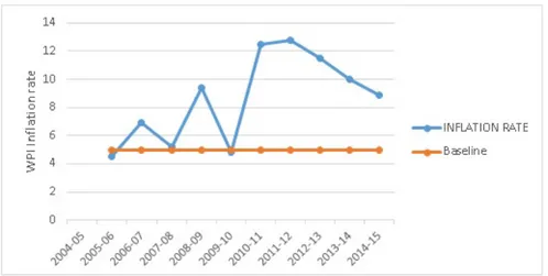
1-1 Annual Rate of Inflation . . . 18

1-2 Stochastic Volatility Plot of Inflation . . . 35

1-3 Stochastic Volatility Plot of Output growth . . . 36

1-4 Stochastic Volatility Plot of Interest Rate . . . 36

1-5 Stochastic Volatility Plot of Crude Oil . . . 36

1-6 Time Varying Simultaneous Relation of Inflation Shock to Output growth . 37 1-7 Time Varying Simultaneous Relation of Inflation Shock to Interest Rate . . 38

1-8 Time Varying Simultaneous Relation of Inflation Shock to Interest Rate . . 38

1-12 IRF of crude oil price shock to inflation in a Constant VAR Model . . . 41

1-13 IRF of inflation shock to output growth in a Constant VAR Model . . . 42

1-14 IRF of inflation shock to output growth in a Time-Varying VAR Model . . . 42

1-15 IRF of output growth to inflation in a Constant VAR Model . . . 42

1-16 IRF of output growth to inflation in a Constant VAR Model . . . 43

1-17 IRF of output growth to inflation in a Time-Varying VAR Model . . . 43

1-18 IRF of crude oil price shock to interest rate in a Constant VAR Model . . . . 43

1-19 IRF of crude oil price shock to interest rate in a Time-Varying VAR Model . 44 1-20 IRF of inflation shock to interest rate in a Constant VAR Model . . . 44

1-21 IRF of inflation shock to interest rate in a Time-Varying VAR Model . . . . 44 1-22 IRF of output growth shock to interest rate in a Time-Varying VAR Model . 45 1-23 IRF of output growth shock to interest rate in a Time-Varying VAR Model . 45

(10)

2-1 Current Account Deficit and Fiscal Deficit Trend in India. . . 52

2-2 Stochastic Volatility Plot of Fiscal Deficit . . . 63

2-3 Stochastic Volatility Plot of Current Account Deficit . . . 63

2-4 Stochastic Volatility Plot of Real Effective Exchange Rate . . . 63

2-5 Stochastic Volatility Plot of Real GDP . . . 64

2-6 Time-Varying Simultaneous Relation of Real GDP shock to FD . . . 65

2-7 Time-Varying Simultaneous Relation of Real GDP shock to REER . . . 65

2-8 Time-Varying Simultaneous Relation of FD shock to REER . . . 65

2-9 Time-Varying Simultaneous Relation of real GDP shock to CAD . . . 66

2-10 Time-Varying Simultaneous Relation of real FD shock to CAD . . . 66

2-11 Time-Varying Simultaneous Relation of REER shock to CAD . . . 66

2-12 Constant Impulse Response Functions/Constant VAR . . . 67

2-13 Time-Varying Impulse Response Functions/Time-Varying VAR . . . 68

3-1 Average Price of Crude Oil in India Note: based on the data of Ministry of Petroleum and Natural Gas (PPAC) . . . 78

3-2 The impulse response functions (IRF) of the variables output growth and Inflation (WPI) to an oil supply shock . . . 84

3-3 The impulse response functions (IRF) of the variables output growth and Inflation (WPI) to an oil demand shock driven by global economic activity 84 3-4 FEVD for India’s GDP, Shock 1: oil supply shock, Shock 2: oil demand shock and Shock 3: oil-specific demand shock . . . 85

(11)

List of Tables

(12)

(13)

List of Abbreviations

AIC Akaike Information Criteria

ARDL Auto Regressive Distributed Lag

BRICS Brazil Russia India China South Africa

BVAR Bayesian Vector Auto Regression

CAD Current Account Deficit

CPI Consumer Price Index

ECM Error Correction Model

FDI Foreign Direct Investment

FD Fiscal Deficit

FRBM Fiscal Responsibility and Budget Management

GCC Gulf Cooperation Council

GDP Gross Domestic Product

HICP Harmonised Index of Consumer Prices

IRF Impulse Response Function

(14)

OECD Organisation for Economic Co-operation and Development

RBI Reserve Bank of India

REER Real Effective Exchange Rate

REH Ricardian Equivalence Hypothesis

STAR Smooth Transition Threshold Auto Regression

SVAR Structural Vector Auto Regression

TV-SVAR Time Varying Structural Vector Auto Regression

TV-VAR Time Varying Vector Auto Regression

US United States

VAR Vector Auto Regression

VECM Vector Error Correction Model

WPI Wholesale Price Index

Nomenclature

C Consumption Expenditure

c crude oil price

C A Current Account

c ag d p current account deficit as a percentage of GDP

f g d p fiscal deficit as a percentage of GDP

(15)

I Investment

i interest rate

l g d p real GDP of India

M Imports

N F Y A Net Factor Income from Abroad

p inflation

R Government transfers

r eer real effective exchange rate

S Savings

Sg Government saving

Sp Personal disposable income

T Taxes

X Exports

x output growth

Gj GDP growth

Pj Price level

Poi l real price of crude oil

Qoi l world oil production

(16)

(17)

Chapter 1 Analysing Inflation in India using

Time-Varying SVAR Model

1.1 Introduction

In today’s world, maintaining low and stable price is essential for improving country’s economic growth. Central Banks devise a framework to fuel the growth of the country. It is a major institution for maintaining economic growth and price stability in a coun-try. Monetary Policy in India is looked after by the Reserve Bank of India (RBI). Recent Monetary Policy in India is driven by multiple objectives like maintaining price stabil-ity, ensuring an adequate credit flow to foster economic growth and financial stability. The relative emphasis on these objectives varies from time to time depending on evolv-ing macroeconomic developments. Consumer Price Index (CPI) data show that India has suffered from chronic inflation for the past five years. In last five years, CPI per-sistently stayed higher than the Central Bank’s limit (which is 5.0%- 5.5%) [22]. For the past decade, we see that the trend line of inflation is high, though it has moved from double digits to a single digit with 8.9% in recent period, it is still not a good sign. For a developing country like India, high inflation is not a good sign for the following reasons:

1. High inflation implies greater burden on average earning people, mainly affects poor. Uncontrolled inflation can lead to distributional inequality in the society.

(18)

Figure 1-1: Annual Rate of Inflation

2. High inflation dries average household savings and decline in overall investment. As a result credit crunch stumbles the economic growth.

3. As inflation rises, high-risk premia in financial markets become prominent. The impact will adversely affect the nominal interest rates. The Higher nominal inter-est rate is a threat to the economy.

4. Higher inflation leads to the appreciation of real exchange rate. Global trade com-petitiveness gets affected through the fluctuations of the currency exchange rate.

1.1.1 Research Problem

Many studies have been carried out to analyse inflation using Time-Varying SVAR ap-proach, in developed countries like Australia, USA and so forth. In recent years, Time-Varying SVAR methodology has been employed in the past studies in Gulf Cooperation Council (GCC) and Brazil Russia India China and South Africa (BRICS). However, very few studies using the applicability of the Time-Varying SVAR approach in understanding the inflation effects in India have been carried out. This approach widens the scope of this chapter. In other words, this chapter tries to check the effect of crude oil price shock on macro variables (output growth and interest rate) and to check how it produces ef-fects in inflation. So the chapter aims to check whether oil price shock has brought

(19)

about any changes in the above-stated macro variables in India. Moreover, the study tests whether the monetary policy mechanisms adopted by the Central Bank has helped in controlling inflation in India. However, in this chapter only those models are looked into which have applied Vector Auto Regression (VAR), Structural Vector Auto Regres-sion (SVAR) and time-varying VAR and SVAR. The chapter mainly focuses on Time Vary-ing Structural Vector Auto Regression (TV-SVAR) approach in understandVary-ing the impact of crude oil price shock on inflation, how RBI responds to this situation and whether RBI has been effective in controlling inflation.

1.2 Literature Review

Most of the countries’ Central Bank target for a low and positive inflation. Persistently high inflation can damage countries economic as well as social growth. Though various models have been employed for understanding inflation dynamics, it is only by the end of late 1990’s that the Time-Varying Vector Auto Regression (TV-VAR) and Time Varying Structural Vector Auto Regression ( SVAR) started gaining importance. In the TV-VAR models proposed in the recent years, we can categorise it into the following three types based on its parameter specification. They are Type 1: Here the parameters are treated as latent variables and are assumed to follow random walks without drifts. The works of Cogley and Sargent [6] [7], Primiceri [19], Canova, Gambetti and Pappa [5], Nakajima, Shiratsuka and Teranishi [16] have employed this technique. Type 2: Here the parameters switch between regimes and are driven by latent state variable which fol-lows a Markov switching process. The work of Sims and Zha [23] is a good example of this category. Type 3: Here the parameters change from one regime to another smoothly (permanently) in time and the specification is the multivariate extension of the Smooth Transition Threshold Autoregression (STAR) model. This technique was developed in the work of He, Terasvirta and Gonzalez [9]. Amongst the three types my chapter fo-cuses on Time-varying parameter SVAR with Stochastic Volatility which falls under Type 1 category.

(20)

1.2.1 Time-Varying Parameter SVAR with Stochastic Volatility

It was Cogley and Sargent [6] who employed three variables (inflation, unemployment and interest rate) and two lags with time-varying coefficients in a VAR model to study the persistence of inflation in the US after World War II. However, this model faced a major limitation i.e. the absence of stochastic volatility. Later Cogley and Sargent [7] im-proved on their previous model by introducing stochastic volatility into the VAR model but with a non-varying structural shock. In other words, this model has drifting co-efficients which allow for changing the variances. This model thus permits stochastic volatility of the shocks, but the contemporaneous responses to shocks do not alter over time. Later Primiceri [19] came up with a model which used three variables namely, inflation, unemployment rate and short-term nominal interest rate with a lag of two periods in time varying SVAR framework to study the Monetary Policy and the Private Sector behaviour of the US economy. In contrast to the work of Cogley and Sargent [7], the framework of his allowed all the parameters to change for the US economy. Fol-lowing the work of Primiceri, many works came up employing the framework of time varying SVAR. Some of these works were like that of Canova, Gambetti and Pappa [5] who used five variables (real output, hours, inflation, federal fund rates and money sup-ply) in time varying SVAR framework to check the dynamics of output growth and infla-tion in the US, euro area and U.K. Benati and Surico [2] employed a time-varying VAR model with stochastic volatility and the following variables (short-term interest rate, in-flation, output growth and money growth to understand the inflation gap persistence in the US economy. Baumeister, Durinck and Peersman [1] used a TVP-VAR model for un-derstanding the effects of excess liquidity shocks on economic activity, asset prices and inflation in the euro area. The variables used in the study were real GDP, HICP consumer prices, short-term interest rate, real asset price index and broad monetary aggregate M3. Later Cogley, Primeceri and Sargent [8] used a time-varying VAR model with drifting co-efficients and stochastic volatility including three variables i.e. inflation, unemployment and the short-term interest rate to understand the inflation gap persistence in the US economy. Nakajima, Shiratsuka and Teranishi [16] employed a TVP-VAR model

(21)

under-standing the effects of monetary policy commitment in the Japanese economy. Again Nakajima, Kasuya and Watanabe [15] had used a Bayesian TVP-VAR model to study the Monetary Policy effect on the Japanese economy. Mumtaz and Sunder-Plassmann [14] used a TVP-VAR to study the time-varying properties of the real exchange rate for the U.K, Eurozone and Canada by taking into account three variables.

However, very few studies using the applicability of the Time-Varying SVAR approach in understanding inflation, through monetary policy transmission mechanism in India have been carried out. It is only by the end of the year 2000 that the applicability of VAR, SVAR and TV-VAR and TV-SVAR models started gaining importance in India. It was Bhat-tacharya and Sensharma [3] who first used SVAR model for understanding the monetary policy signals in pre and post Liquidity Adjustment Facility (LAF) period in India using SVAR model. In the pre-LAF period, they found that CRR performed better than RBIâ ˘A ´Zs signalling target Bank Rate. In post LAF period the repo and reverse repo rate were iden-tified to be effective instruments of signalling in money, bond and forex market. How-ever, it remained unaffected in the stock market. Later Biswas, Singh and Sinha [4] built a model to forecast inflation in India and also the Index of Industrial Production (IIP) growth using Bayesian Vector Autoregression (BVAR) model. Authors claim that their prediction made with BVAR framework is better than making predictions through VAR model. In a study of Patnaik [18], to identify the major causes of inflation in India using a VAR model she concludes that inflation in India could be found to be mainly demand driven. The supply side effects persist, but it is not sustainable. The author argues for a better stabilisation policy. Mallick [11] in his paper used an SVAR approach to captur-ing the macroeconomic effects of monetary policy in the Indian context. He found that supply shocks were the dominant source of inflation and interest rate play a better role in stabilising inflation in India than the exchange rate. Later, Mishra and Mishra [12] tried to capture the monetary transmission mechanism for Indian economy by using VAR approach. Their results suggest that demand effects of interest rate are stronger than the exchange rate effects. The paper also shows the potential conflict between ex-change rate and the interest rate, which acts as a primary concern for inflation targeting in India. The work of Kumar, Srinivasan and Ramachandran [10] became significant as

(22)

they tried to build a model of inflation using time varying parameter for India. To de-termine the dynamics of inflation they used RBI’s preferential parameters and the slope of Phillips Curve. The model is estimated using the median -unbiased estimator. They conclude that exchange rate and good luck helped in inflation reduction while monetary policy and structural change have played a non-trivial role. However, it was Mohanty and John [13] who first employed Time-varying SVAR with stochastic volatility approach to examine the factors that may have contributed to inflation in India. Crude oil prices, output gap, fiscal policy and monetary policy were taken as the variables other than in-flation for their study. They conclude by saying the drivers of inin-flation are frequently changing in India and also comment that the role of monetary and fiscal policy to con-tain the inflation has failed, irrespective of the nature of the shock to inflation.

1.3 Methodology

The paper focuses on the usage of Time-Varying SVAR model for the following reasons:

1. A large number of studies have been carried out on the transmission of monetary policy shocks using SVAR models. The role played by changes in the volatility of these shocks has been ignored in the existing SVAR model. The studies do allow time-varying shock volatility, but do not incorporate a direct impact of the shock variance on the endogenous variables. But, Time-Varying SVAR model helps to overcome this problem. (Mumtaz and Sunder-Plassmann, [14]).

2. The model must include time variations of the variance and covariance matrix of the innovations, to make changes in policy, structure and their interactions. This reflects both time variation of the simultaneous relations among variables of the model and heteroscedasticity of the innovations. This could be done by develop-ing a multivariate stochastic volatility modelldevelop-ing strategy for the law of motion of the variance and covariance matrix. This could also be stated as the advantage of the Time-Varying SVAR model compared to the other models (Primiceri E Gior-gio, [19]).

(23)

3. TV-SVAR models are faster in capturing the structural changes in inflation than the rolling VAR models. The TV- VAR models are far superior to the VAR models (K. Triantafyllopoulos, [24]).

1.3.1 The Basic Model

Let us consider a simple VAR model with constant parameters and with no restriction on the AR lag structure.

Ay_t = F1y_{t −1}+ ... + Fsy_{t −s}+ ut (1.1)

where y_t denotes a k × 1 vector of variables with a lag length of ‘s’, A is the matrix of contemporaneous coefficients while F1, F2, ..., Fsare the matrices of coefficients, ut is

assumed to have mean 0 and fixed variance-covariance matrixΣ. The structure of the matrix A is A =          1 0 · · · 0 α21 1 · · · 0 · · · · αk1 αk2 · · · 0         

In other words, the equation could be rewritten as

yi ,t= x

0

i ,tβt+ ui ,t i = 1,...,n t = 1,...,T (1.2)

where yi ,t denotes the observation on the variable i at time t, xi ,t is a k-vector of

lagged dependent explanatory variables. Considering all the endogenous variables jointly Eq.(1.2) looks like

y_t= X0tβ + ut (1.3)

where y_t =£ y1t, y2t, . . . , ynt

¤0

(24)

y_t=          y_1,t y_2,t .. . y_n,t          X0_t=          x0_1,t 0 · · · 0 0 x0_2,t . .. ... .. . . .. ... 0 0 · · · 0 x0_n,t          β=          β1 β2 .. . βn          ut=          u1,t u2,t .. . un,t         

Now considering a model with time-varying parameters and no restriction on the AR lag structure Eq.(1.2) can be written as:

y_{i ,t}= x0i ,tβi ,t+ ui ,t i = 1,...,n t = 1,...,T (1.4)

Here yi ,t denote the observation of variable i at time t. Let xi ,t be a k-vector of

ex-planatory variables in equation Eqt.(1.4). Now considering all the yi ,t’s jointly Eq.(1.3)

looks like:

yt= X

0

tβt+ ut (1.5)

Here y_{i ,t} denote the observation of variable i at time t. Let xi ,t be a k-vector of

ex-planatory variables in Eq.(1.5). Now considering all the y_{i ,t}’s jointly in Eq.(1.5) looks like1: y_t=          y_1,t y_2,t .. . y_n,t          X0_t=          x0_1,t 0_1×k2 · · · 0_1×kn 0_1×k1 x0_2,t . .. ... .. . . .. . .. 0_1×kn 0_1×k1 · · · 0_1×kn−1 x0_n,t          βt=          β1,t β2,t .. . β_n,t          ut=          u1,t u2,t .. . un,t         

The vector of innovations ut is assumed to have a multivariate normal distribution

with mean zero and a covarianceΩt i.e. ut∼ (0,Ωt). This matrix can be decomposed

using a triangular factorization i.e. AtΩtA

0

t =Σt Σ

0

t 2where At andΣt are n × n matrices

having the following structure.

1_{for better explanation see Appendix A} 2_{See the Appendix A for explanation}

(25)

At=          0 · · · 0 α21,t 1 . .. ... . .. .._. _{. ..} ₀ αn1,t · · · αnn−1,t 1          Σt=          σ1,t 0 · · · 0 0 σ2,t · · · 0 0 . .. ... ... 0 · · · 0 σn,t         

Assuming ut= A−1t Σtεt,εt where is a n-vector whose components have independent

univariate normal distribution. Thus Eq.(1.5) can be rewritten as:

yt = ct+ B1,tyt −1+ ... + Bk,tyt −k+ ut (1.6)

This model was employed in the work of Primeceri [19], Cogley and Sargent [6], [7] and Nakajima [17]. However, these models had some differences which are explained below briefly by comparing each of these models.

COGLEY AND SARGENT [6]

The aim of this paper was to provide evidence for the evolution of measures of the persistence of inflation, prospective long-horizon forecasts (means) of inflation and un-employment. The model has also employed three variables. (Inflation, unemployment and the real interest rate) Moreover, two lags for estimation. The data for the sample spans from 1948: Q1 to 2000: Q4. The primary results were that there was a long run mean, persistence and variance of inflation have changed. The Taylor principle was vio-lated before Volcker (pre-1980) and the monetary policy was too loose. The model could be explained as follows: The measurement equation used is similar to Eq.(1.5) stated above i.e.

yt= X

0

tθt+ εt (1.7)

Here y_t is a n-vector of endogenous variables. θt is a k vector of coefficients. X

0

t is a

n × k matrix of predetermined/exogenous variables and εt is a n × 1 vector of prediction

errors. The vector y_t includes inflation and other variables that are useful for predicting inflation. The coefficients of VAR are considered as a hidden state vector and the state vectorθt are postulated to evolve according to:

(26)

ρ(θt +1| θt,V ) ∝ I (θt +1) f (θt +1| θt,V ) (1.8)

With I(θt)= 0, if the roots of the associated VAR polynomial are inside the unit circle

and 1 otherwise. V is the covariance matrix defined as:

f (θt +1| θt,V ) ∼ N (θt,Q) (1.9)

Eq.(1.9) is represented as the driftless random walk, which becomes the transition equation such as

θt= θt −1+ vt (1.10)

Here vt is an i.i.d Gaussian process with mean 0 and covariance Q. the innovations

(ε0_t, vt0) are assumed to be i.i.d with zero mean and covariance matrix.

Et= ¡ε_t vt ¢h ε0 t , v 0 t i = V =   R C0 C Q  

R is a n × k covariance matrix for the measurement innovations, and Q is the k × k

covariance matrix for the state innovations, and C is a k × n covariance matrix. The authors use Bayesian methodology soθt’s are parameters, and the elements R, Q and C

are treated as hyperparameters.

PRIMICERI [19]

The paper studies the changes in the monetary policy in the US over the post-world war period. There are three variables employed namely inflation, unemployment and real interest rate and two lags have been used for estimation. The data is from 1953: I to 2001: III. The main results were that the systematic responses of the interest rate to inflation and unemployment trend toward a more aggressive behaviour and this had a negligible effect on the rest of the economy. The model could be explained as follows:

The model follows Eq.(1.6) and is written as:

(27)

The VAR’s time-varying parameters collected in the vector y_tare postulated to evolve according to

ρ(θt | θt −1,Q) ∝ I (θt) f (θt| θt −1,Q) (1.12)

with I (yt) being an indicator function rejecting unstable draws thus enforcing a

sta-tionarity constraint on the VAR and with f (θt| θt −1,Q) given by:

θt= θt −1+ ηt ηt∼ N (0,Q) (1.13)

The time-varying matrices Ht and At are defined as

Ht=       h1t 0 0 0 h2t 0 0 0 h3t       At=       1 0 0 α21,t 1 0 α31,t 0 1       (1.14)

With hi ,t evolving as geometric random walks, lnhi ,t = lnhi ,t −1+vi ,t.

ht is defined as ht=[ h1,t, h2,t, h3,t, h4,t ¤0

the non zero and non-one elements of the matrix At, are postulated by collecting in the vectorαt=[α21,t, ...αn1,t, ...αnn−1,t

¤0

to evolve as driftless random walks. This model has drifting coefficients and a fully varying covari-ance matrix. It permits changes in the contemporaneous responses to standard shocks, which is in accordance with the lower triangular structural VAR. To compute the spec-ification, the elements below the main diagonal of At are stacked by rows into an

n(n-1)/2×1. Vector αt=[α21,t, ...αn1,t, ...αnn−1,t

¤0

. Vectorωt=[ logσ_1,t, ..., logσn,t

¤0 .

Thus the dynamics of the time varying parameters are determined by the following state of equations:

βt= βt −1+ γt γt∼ N (0,Q)(1.15)

αt= αt −1+ ζt ζt ∼ N (0,Q)(1.16)

(28)

Eq.(1.15)-Eq.(1.17) clearly explains the random walk structure of the TV Parameter. Here the covariance matrices Q and W of the vectors of state innovationγ_tandη are left unrestricted but the covariance matrix S of the vector of state innovationsζt is assumed

to be block diagonal with blocks corresponding to different rows of At. The joint

distri-bution of the innovations is postulated as [ logσ_1,t, ..., logσ_n,t¤0 [εt,γt,ζt,ηt]

0

∼ N(0,VA)

where VAis assumed to be block diagonal with blocks In, Q, S and W.

Thus when a comparison is made between Cogley and Sargent [6] and Primeceri [19], we find that in the former there are drifting coefficients but a fixed covariance matrix of the innovations. This rules out any changes in the variances or contemporaneous responses to the shocks. It is based on Eq.(1.2). The coefficients are assumed to fol-low Eq.(1.12), but the covariance matrix of the observation innovations is constant i.e.

Ωt=Ω,t= 1...T. The joint distribution of innovations is postulated [ut, γt]

0

∼ N (0, VC)

where the matrix VCis assumed to be block diagonal with blocksΩ and Q.

COGLEY AND SARGENT [7]

This paper was an improvement over the paper of Cogley and Sargent [6]. The pre-vious model faced a major limitation of the absence of stochastic volatility. This paper improved on this by introducing stochastic volatility into the VAR model, but with a non-varying structural shock. The model is based on Eq.(1.6). The model could be explained as follows:

The measurement equation used is Eq.(1.7) and the transition equation used is Eq. (1.10). In Eq.(1.7) y_tis a vector of endogenous variables, Xt includes a constant plus lags

of y_tandθtis a vector of VAR parameters. In the measurement equation Xt= InN xtand

xt includes all the regressors (i.e. lags of yt as well as the constant). Thus the

measure-ment equation could be rewritten as:

yt= Θtxt+ εt (1.18)

Here the relationship betweenΘt andθt is given byΘt= vecθ

0

t. The innovations vt

(29)

distributed with the variance that evolves over time: εt∼ N (0, Rt) (1.19) With Rt= B−1H−1t 0 (1.20) Here B is lower triangular matrix with ones on the diagonal and Htis a diagonal with

elements that vary over time according to drift less, geometric random walk.

ln hi ,t= ln hi t −1+ σiηi ,t (1.21)

Now when the Eq.(1.15) is pre-multiplied by B we obtain

Byt = Btxt+ ut (1.22)

Where Bt= BΘt which are the structural form coefficients and ut= Bεt is a vector

of uncorrelated errors. Let at be defined as vec(B

0

t)= (BN Ip)θt where p is the number

of regressors in each equation. Pre multiplying Eq.(1.7) by BN Ip gives the transition

equation for structural parameters which is also a random walk:

at= at −1+ ˜vt, ˜vt ∼N(0, ˜Q) with ˜Q= (BN Ip) Q (BN Ip). Since Q is unrestricted in this

work of Cogley and Sargent this transformation does not alter any assumption. Thus, this model has drifting coefficients but only allows for changing the variances. This model thus permits stochastic volatility of the shocks but the, contemporaneous re-sponses to shocks do not change over time. The coefficients and the log standard de-viations are assumed to follow Eq.(1.15)-(1.17), but it is assumed that At=A, t= 1...T. The

joint distribution of innovations is postulated as [εt,γt,ηt]

0

∼ N (0, VB) where matrix VB

is assumed to block diagonal with blocks In, Q and W.

Nakajima [17]

The work carried out by Nakajima to analyse the monetary policy commitment in Japan using three variables namely inflation, output and interest rates3. In the previous

3_{The study used two types of interest rates, namely short-term interest rates and medium-term interest}

(30)

works, it is noticed that the time-varying coefficients were only capturing temporary shifts in the coefficients. However, in the methodology employed by Nakajima the time-varying coefficientsαt captures both the temporary and permanent shifts in the

coef-ficients. In other words, a structural break is also being captured in this methodology. The TVP model is as follows:

yt = x 0 tβ + z 0 tαt+ εt, εt ∼ N(0, σ2t), t = 1,...,n (1.23) αt +1= αt+ ut, ut∼ N(0, Σ) (1.24) σ2 t = γexp(ht), ht +1= φht+ ηt, ηt∼ N(0, σ2t), t = 1,...,n − 1 (1.25)

Here Eq.(1.23) is a regression equation where yt is a scalar of response, x

0

t and z

0

t are

k × 1 and p × 1 vectors of covariances respectively. In this equation there is a constant

co-efficient and time-varying co-efficient. The constant co-efficient is β which is a k vector and the time-varying co-efficient isαt which is a p vector. The effects of xt on yt

are assumed to be time-invariant, while the regression relations of zt to yt are assumed

to change over time.

In Eq.(1.24) the time-varing coefficientsαtare assumed to follow first-order random

walk process. In other words , we can say thatαt captures both the temporary and

per-manent shifts in the coefficients. Eq.(1.25) captures the stochastic volatility. Here the log-volatility, htis modelled to follow AR(1) process in the equation. This has been done

to avoid the spurious movements ofαt. In other words, it can be said that the

station-ary condition is assumed in the following equation asηt ∼ N(0, σ2t). Moreover,φ is also

assumed as |φ|< 1. The disturbance of the regression is εt, which follows a normal

distri-bution with time-varying variancesσ2_t as shown in Eq.(1.23). In crux Eq.(1.23)-Eq.(1.25) are assumed to follow the following assumptions:

1. α0= 0 2. u0∼ N(0, Σ)

(31)

3. γ > 0

4. ht = 0

After having a survey of all the works employing time-varying VAR, the analytical framework of the proposed study would be based on the methodology followed by Naka-jima [17]. The analytical framework is explained in the next section.

1.3.2 Analytical Framework (TV-SVAR with Stochastic Volatility)

To understand the impact of crude oil price shock on macro variables and to check how it produces dynamic effects in inflation in India, the study employs a four-variable VAR. It includes inflation (p), output growth (x), interest rate (i)4and crude oil prices (c)5[25]. Here inflation is calculated based on Whole Sale Price Index (WPI). The data on infla-tion and output growth is obtained from the Reserve Bank of India (R.B.I) website [20]. The data for crude oil is obtained from the World Bank data on international commodi-ties [23]. The data employed is quarterly data Q1:1996 to Q4: 2013. The lag of 2 periods is taken based on Akaike information criteria(AIC). Hence there is a possibility of sea-sonality in the data set. This issue is tackled by using cubic spline methodology. The data uses WPI, as the measure of inflation for the following reasons:(i) WPI has a wider coverage of items compared to CPI and is much more directly affected by international commodity prices in comparison to CPI. This study tries to understand whether oil price shock has brought about any change in the macro variables and crude oil price is an in-ternational commodity. (ii) Data on WPI is available on a weekly basis in comparison to CPI data. Thus the data on WPI helps us to capture the impact of shocks better. (iii) During the present study period, the RBI did not change the inflation measure from WPI to CPI. Thus to capture the effectiveness of the policy decisions taken the study resort to WPI as a measure. Thus, Time-Varying Impulse Response Function (IRF) is used to check whether oil price shock has brought about changes in the macro variables stated above. Using the Time-Varying IRF we check the following:

4_{Here interest rate refers to nominal interest rate} 5_{Here crude oil prices refer to the World Brent Oil Prices}

(32)

1. Impact of crude oil price shock to inflation. 2. Impact of crude oil price shock to output growth. 3. Impact of inflation shock to output growth.

4. Impact of crude oil price shock on the interest rate. 5. Impact inflation shock on the interest rate.

6. Impact of output growth shock to the interest rate.

The Structural identification restriction for SVAR are estimated as follows:

1. Crude oil price is considered to be exogenous to the framework.

2. Inflation is said to respond immediately to the crude oil prices and with output growth and interest rate with a lag of one period.

3. Output growth is sensitive to interest rate and inflation. 4. Interest rate is sensitive to output growth and inflation.

Yt is a n-vector of the following 3 variables [πt,xt,it] at time t with crude oil prices

(ct) considered to be be exogenous to the system. The structural identifications are

in-corporated into Eqt.(1.1)6. Following Eqt.(1.1) - (1.6), the TVP -VAR is formulated on Nakajima’s work [17] as follows7:

yt = ct+ B1tyt −1+ B2tyt −2+ B3tyt −3+ ut (1.26)

Here ut= A−1t Σtεt. Thus the equation could also be rewritten as follows:

yt = ct+ B1tyt −1+ B2tyt −2+ B3tyt −3+ A−1t Σtεt (1.27)

Here y_t= X0tβt where in the case of B1t the expansion will be as follows:

6_{See the Appendix A for the structural identification imposed on the variables.} 7_{Refer Appendix A for the software and package information}

(33)

B1t=          b11 b12 b13 · · · b1n b21 b22 b23 · · · b2n .. . ... ... · · · ... bn1 bn2 bn3 · · · bnn          1t =          b0₁ b0₂ .. . b_n0          1t =          b₁0, 1t b₂0, 1t .. . b_n0, 1t          Xt=          1y0_{t −1} 0 0 · · · 0 0 1y0_{t −1} 0 · · · 0 0 0 1y_{t −1} · · · 0 0 0 0 · · · 1y_{t −1}          β=                    c1 b1, 1t c2 b2, 1t .. . cn bn, 1t                   

In this similar manner B2t and B3t will be formulated. Thus we can say that Bt =

[vec(B 1, t )0, vec(B 2, t )0, ..., vec(B n, t )0]. Other than these the parameters in Eq.(1.27) fol-low a random walk process as folfol-lows:

β_{t +1}= βt+ uβt, at +1= at+ uat, ht +1= h + uht(1.28)          εt u_βt uat uht          ∼ N          0,          I 0 0 0 0 Σ_β 0 0 0 0 Σa 0 0 0 0 Σht                  

for t=s + 1,...,n, where β_s+1∼ N (µβ0,Σβ0), as+1∼ N (µa0,Σa0) and hs+1(µh0,Σh0).

Other than this the TVP-VAR model has the following properties

(34)

of lower-triangular elements in At and ht +1=(h1t,...,hkt)

0

with hj t=logσ2_{j t} for j =

1, ..., k, t = s + 1.

2. The parameters are not assumed to follow a stationary process such as AR(1), but the random walk process.

3. The variance and covariance structure for the innovations of the time-varying pa-rameters are governed by the papa-rameters,Σβ,ΣaandΣh.

4. Prior is set for the random walks. The prior distribution of the variance-covariance matrix is assumed to follow inverse-Wishart. The prior distribution of the initial states of time varying coefficients is assumed to be normally distributed. This is estimated using Gibbs sampling in (Markov Chain Monte Carlo) algorithm.

1.4 Results

The study focuses on the usage of time-varying Impulse Response Function(TV-IRF) with stochastic volatility following the methodology of Nakajima [17] to analyse the im-pact of crude oil price (c) shock on inflation (p), output growth (x) and the interest rate

(i). First, the stochastic volatility is plotted for all the variables. The stochastic

volatil-ity helps in understanding the significant spike periods. Secondly, the Time- Varying Simultaneous Relations of all the variables are plotted. The Time- Varying Simultane-ous Relations helps in understanding the relationship between the different variables employed. Next, the impulse response functions are calculated. Here IRFs is estimated by fixing the initial shock as the average of stochastic volatility measure for each vari-able and using the simultaneous relations at each point. The estimated time varying coefficients are used to compute the IRFs from the current to future periods. Finally, the impact of the variables in a VAR and Time-Varying SVAR model are compared us-ing an Impulse Response Function (IRF). This comparison is made to understand the significance of using a TV-SVAR model to understand the impact of an oil shock on the specified macro variables.

(35)

Figure 1-2: Stochastic Volatility Plot of Inflation

1.4.1 Stochastic Volatility Plot

In figure 1.2 the stochastic volatility plot of inflation is considered. Here the spike could be seen in the year 2009. The reason for the spike could be attributed to the global fi-nancial crises of 2008, as a result of which the prices are said to increase. In figure 1.3 the stochastic volatility plot of output growth is considered. Here we see two spikes, one in the year 2006 and the other in the year 2009. The spike in 2006 is a positive out-put growth spike as the Foreign Direct Investment (FDI) inflows stood at 5.5$ billion in 2004 [25]. This made India be the 10th largest regarding overseas investment received. However, the spike in 2009 is for a negative output growth which happened gain due to the global financial crises. In the case of interest rate, we see two spikes which are seen increasing from the year 2000 with a huge fluctuation in 2009. Here again, the severe impact of the global financial crisis could be found. According to the Monetary Policy Report of 2013 [21] the interest rate recorded it’s highest and lowest interest rates in the following years were the spikes are depicted. This could be observed from figure 1.4. In figure 1.5 we find that there are two stochastic volatility spikes for crude oil price. Around 2001, the spike could be attributed to multiple issues such as the 9/11 attacks and the uncertainties surrounding major economies. Further, the collapse of the dot com bub-ble may be also taken into consideration.The spike around 2009 could be attributed to the oil price collapse after the 2008 financial crisis.

(36)

Figure 1-3: Stochastic Volatility Plot of Output growth

Figure 1-4: Stochastic Volatility Plot of Interest Rate

(37)

Figure 1-6: Time Varying Simultaneous Relation of Inflation Shock to Output growth

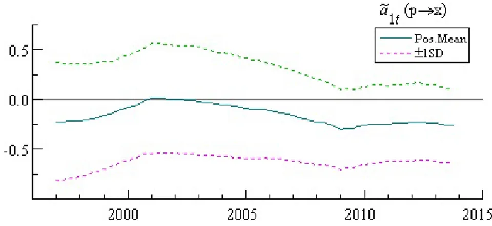
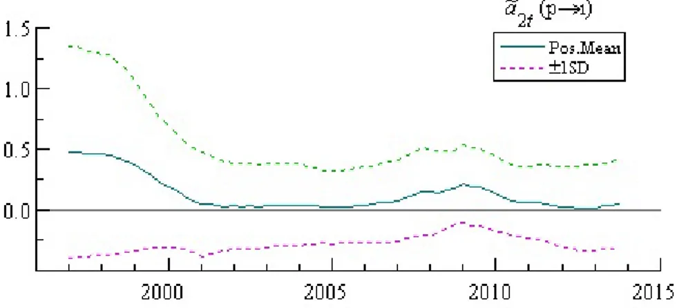
1.4.2 Time - Varying Simultaneous Relation

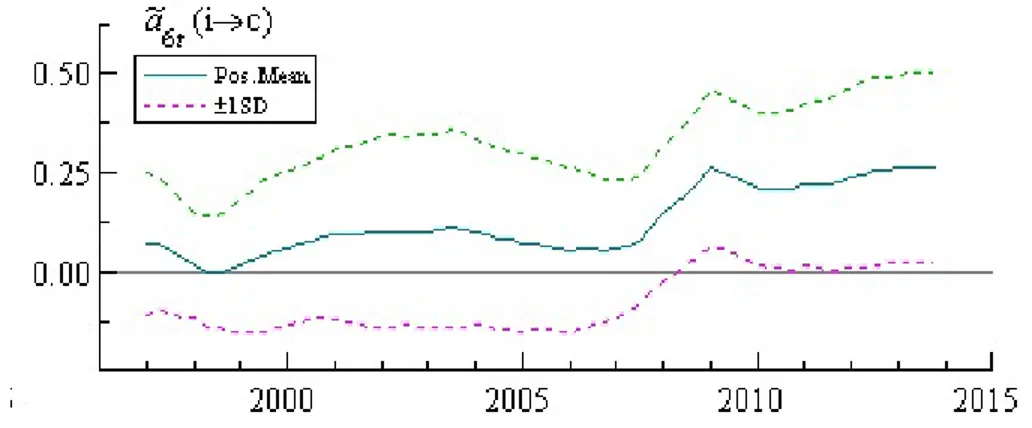
Next, the time varying simultaneous relation, a salient feature of TVP-VAR is analysed. In figure 1.6 the time varying simultaneous relation of inflation shock to output growth is observed. Here it is noted that the simultaneous relation of the shock of inflation to output growth remains negative throughout the period. In figure 1.7 the time varying simultaneous relation of inflation shock to interest is observed. It is found that interest rates remain positive throughout the period. In figure 1.8 the shock of output growth to interest rate is considered. It is found that the shock of output growth to interest rate remains positive till 2004 later fluctuates and becomes positive after 2005. In other words, the simultaneous relation of the interest rates to output growth shock vary over time. This is similar to the shock of inflation to crude oil remains as it varies throughout the period of analysis. This is seen in figure 1.9. The shock of output growth to crude oil price remains negative till 2008 and becomes positive after 2008 in response to the global financial crises.In other words, we can say that in figures 1.10 the simultaneous relation of output growth to crude oil price vary over time. While the shock of an interest rate to crude oil price is positive with fluctuations and making it at a high positive rate after 2008, in responses to the global financial crises. This could be observed in figure 1.11.

(38)

Figure 1-7: Time Varying Simultaneous Relation of Inflation Shock to Interest Rate

(39)

(40)

1.4.3 Time - Varying Impulse Response Functions and Comparison with

VAR Models

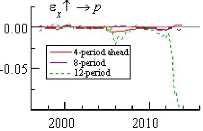
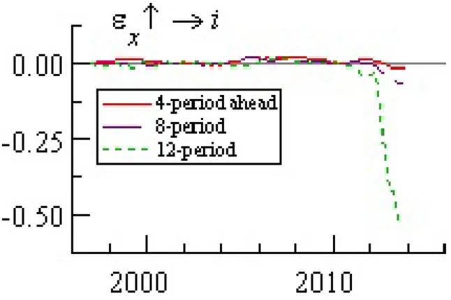
Next, the impulse response functions are calculated. Here IRFs is estimated by fixing the initial shock as the average of stochastic volatility measure for each variable and using the simultaneous relations at each point. The estimated time varying coefficients are used to compute the IRFs from the current to future periods.The time-varying IRFs will also be compared with the constant VAR models to understand the advantage of a time-varying model. In time-time-varying IRF we have a short, medium and long-term forecast. The short term is for four quarters. The medium term is for eight quarters ahead, and the long term impact is for 12 quarters ahead period.

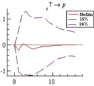
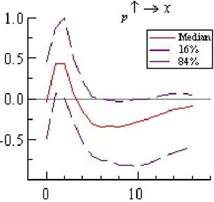
The time varying IRFs are estimated by showing the size of responses from a four period ahead of the horizon for a 12 period ahead of the horizon. Firstly the IRF of a crude oil price shock to inflation in a VAR and Time-Varying VAR model is analysed.In figure 1.12 it is found that the impact of crude oil price shock to inflation is negative throughout the period of study in a constant VAR Model. However, the impact of crude oil price shock to inflation is initially positive but becomes negative during the third period varying VAR Model. This is clearly seen in figure 1.13. But the impact of inflation shock to output growth is same in both the VAR and time-varying VAR Model. This is clearly evident from figure 1.14 and figure 1.15. In other words, when the response of output growth to one SD shock in inflation is analysed in time varying IRF, initially in the first period, it is positive while it continues to become negative from the second to the third period. Similarly, in a constant VAR Model, it could be found that the result obtained is similar, i.e., Initially, it is positive but comes negative at a later period. When the impact of output growth to inflation is made, the results obtained in a constant VAR Model and time- varying VAR Model differ. In a constant VAR Model, the response is found to be negative throughout the period, as seen in figure 1.16. However in time-varying VAR Model, initially in the first period, it is positive while it continues to become negative from the second to the third period as seen in figure 1.17. When the impact of Crude oil price shock to interest rate is analysed in time-varying VAR Model, we find

(41)

Figure 1-12: IRF of crude oil price shock to inflation in a Constant VAR Model

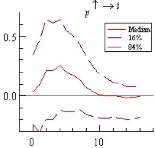
that initially the interest rate responds immediately by increasing and later increasing at a declining rate. In other words, it becomes negative from the four years ahead of the horizon as seen in figure 1.19. This is similar to the result obtained in a constant VAR Model as seen in figure 1.18 where the response is seen increasing at a declining rate. However, the impact of inflation shock to interest rate is initially negative and tends to be positive for the next two periods as seen in figure 1.21 for a time-varying VAR. But, in the constant VAR Model, the impact is found to be positive throughout the period, as seen in figure 1.20. In figure 1.23 the impact of output growth shock to interest rate is analysed. The impact of the output growth shock to interest rate is positive for the first two periods but tends to be negative by the end of the third period in a time-varying model. But for a constant VAR model the impact is found to be negative as seen in figure 1.22.

1.5 Conclusion

From the results obtained above, we could clearly see the difference in using a time -varying VAR model in comparison with a constant VAR Model. It is evident from the results that time - varying VAR Model is more sensitive in capturing results compared to a constant VAR Model. When the policy initiative is analysed, we find that the

(42)

imme-Figure 1-13: IRF of inflation shock to output growth in a Constant VAR Model

Figure 1-14: IRF of inflation shock to output growth in a Time-Varying VAR Model

(43)

Figure 1-16: IRF of output growth to inflation in a Constant VAR Model

Figure 1-17: IRF of output growth to inflation in a Time-Varying VAR Model

(44)

Figure 1-19: IRF of crude oil price shock to interest rate in a Time-Varying VAR Model

Figure 1-20: IRF of inflation shock to interest rate in a Constant VAR Model

(45)

Figure 1-22: IRF of output growth shock to interest rate in a Time-Varying VAR Model

(46)

diate response of crude oil price shock to inflation is that inflation rises in one-quarter period ahead, followed by a decline in inflation after four quarter period. The output growth immediately responds by becoming negative and later becomes negative at a lesser rate during the four quarter period ahead. The inflation shock makes output growth to respond quickly by becoming positive and subsequently becomes negative after four quarter period. The interest rate responds immediately by increasing at a pos-itive rate, which continues even after4 quarters. From the results obtained we could conclude that a crude oil prices shock is followed by an increase in inflation. Later the inflation shocks respond to output growth with a decline in output growth. The R.B.I re-sponds to this situation by raising the interest rate, and we see inflation reaching stability rates after this. Thus we can conclude that the monetary policy is effective in controlling inflation in India, to some extent.

(47)

Bibliography

[1] Baumeister, C., Durinck, E. and Peersman, G., 2008. Liquidity, inflation and asset prices in a timevarying framework for the euro area. NBB Working Papers. No. 142, 16 October 2008.

[2] Benati, L. and Surico, P., 2008. Evolving US monetary policy and the decline of inflation predictability. Journal of the European Economic Association, 6(2â ˘A ˇR3), pp.634-646.

[3] Bhattacharyya, I. and Sensarma, R., 2008. How effective are monetary policy signals in India?. Journal of Policy Modeling, 30(1), pp.169-183.

[4] Biswas, D., Singh, S. and Sinha, A., 2010. Forecasting inflation and IIP growth: Bayesian vector autoregressive model. Reserve Bank of India Occasional Papers, 31(2), pp.31-48.

[5] Canova, F., Gambetti, L. and Pappa, E., 2007. The structural dynamics of out-put growth and inflation: some international evidence. The Economic Journal, 117(519), pp.C167-C191.

[6] Cogley, T. and Sargent, T.J., 2002. Evolving post-world war II US inflation dynamics. In NBER Macroeconomics Annual 2001, Volume 16 (pp. 331-388). MIT Press. [7] Cogley, T. and Sargent, T.J., 2005. Drifts and volatilities: monetary policies and

out-comes in the post WWII US. Review of Economic dynamics, 8(2), pp.262-302. [8] Cogley, T., Primiceri, G.E. and Sargent, T.J., 2010. Inflation-gap persistence in the

(48)

[9] He, C., Terasvirta, T. and Gonzalez, A., 2008. Testing parameter constancy in sta-tionary vector autoregressive models against continuous change. Econometric Re-views, 28(1-3), pp.225-245.

[10] Kumar, S., Srinivasan, N. and Ramachandran, M., 2012. A time-varying parameter model of inflation in India. Indian Growth and Development Review, 5(1), pp.25-50.

[11] Mallick, S., 2009. Macroeconomic Shocks, Monetary Policy and Implicit Excahnge Rate Targeting in India. Mimeo, Queen Mary University of London.

[12] Mishra, A. and Mishra, V., 2012. Evaluating inflation targeting as a monetary policy objective for India. Economic Modelling, 29(4), pp.1053-1063.

[13] Mohanty, D. and John, J., 2015. Determinants of inflation in India. Journal of Asian Economics, 36, pp.86-96.

[14] Mumtaz, H. and Sunder-Plassmann, L., 2013. Time-Varying Dynamics of the Real Exchange Rate: An Empirical Analysis. Journal of applied econometrics, 28(3), pp.498-525.

[15] Nakajima, J., Kasuya, M. and Watanabe, T., 2011. Bayesian analysis of time-varying parameter vector autoregressive model for the Japanese economy and monetary policy. Journal of the Japanese and International Economies, 25(3), pp.225-245. [16] Nakajima, J., Shiratsuka, S. and Teranishi, Y., 2010. The effects of monetary policy

commitment: Evidence from time-varying parameter VAR analysis (No. 10-E-06). Institute for Monetary and Economic Studies, Bank of Japan.

[17] Nakajima, J., 2011. Time-varying parameter VAR model with stochastic volatility: An overview of methodology and empirical applications (No. 11-E-09). Institute for Monetary and Economic Studies, Bank of Japan.

[18] Patnaik, A., 2010. Study of inflation in India: A cointegrated vector autoregression approach. Journal of Quantitative Economics, 8(1), pp.118-129.

(49)

[19] Primiceri, G.E., 2005. Time varying structural vector autoregressions and monetary policy. The Review of Economic Studies, 72(3), pp.821-852.

[20] India, R.B.O., 2012. Reserve Bank of India. Handbook of Statistics on the Indian Economy, RBI Database. https://dbie.rbi.org.in/DBIE/dbie.rbi? site=publications

[21] India, R.B.O., 2013. Reserve Bank of India. Monetary Policy Report, April 2013. [22] India, R.B.O., 2015. Reserve Bank of India. Monetary Policy Report, April 2015. [23] Sims, C.A. and Zha, T., 2006. Were there regime switches in US monetary policy?.

The American Economic Review, 96(1), pp.54-81.

[24] Triantafyllopoulos, K., 2008. Forecasting with time-varying vector autoregressive models. arXiv preprint arXiv:0802.0220.

[25] United Nations Conference on Trade and Development., 2006 . World Investment Report, FDI from Developing and Transition Economies:Implications for Develop-ment.

[26] The World Bank., 2012. World Bank Commodities Price Data (The PinkSheet), Crude Oil, Brent http://www.worldbank.org/en/research/ commodity-markets.

(50)

(51)

Chapter 2 Twin Deficit Hypothesis and its

Relevance in India: Time-Varying VAR

Approach

2.1 Introduction

The impact of the budget deficit in developing countries, is a topic that is highly debated nowadays, as the effect of it depends on the response of trade deficit to changes in the fiscal shocks. In other words, we can say that budget deficit and trade deficit are interre-lated, through the phenomena called twin deficit hypothesis. Maintaining a sustainable budget deficit is thus considered as a necessary condition for the maintenance of a com-fortable level of current account balance. However, there exist views that are supporting as well as rejecting twin deficit hypothesis. The view supporting twin deficit hypoth-esis states that budget deficit leads to a trade deficit. Studies conducted by Abell [1], Zietz and Pemberton [43], Bachman [10], Kasa [19], Vamvoukas [40], Cavallo [12] and Erceg et al.[16] confirms this claim. Moreover, they also found that the budget deficit is a significant cause of the trade deficit. However, the Ricardian Equivalence Hypothesis (REH) denies this claim. In other words, REH argues that the two deficits are not twins. Studies conducted by Enders and Lee [15], Boucher [11], Winner [41], and Kaufmann,

(52)

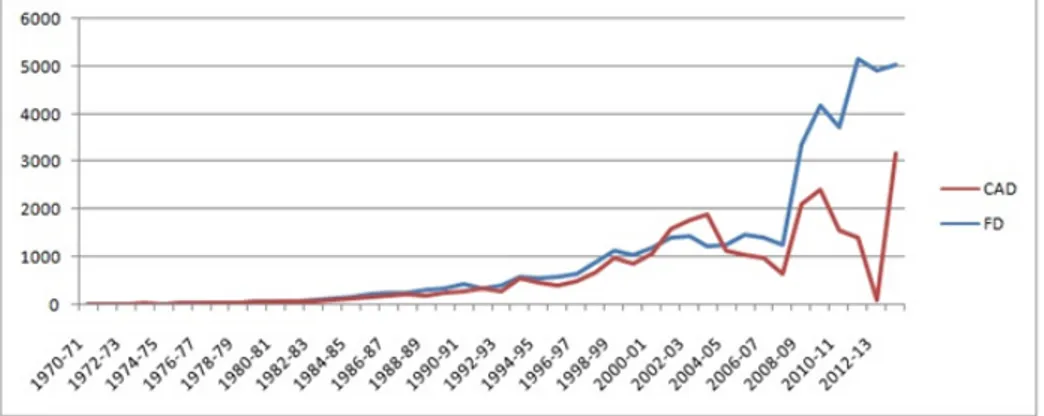
Figure 2-1: Current Account Deficit and Fiscal Deficit Trend in India.

Johan and Georg [20], are some examples that validate this claim. In the Indian con-text, it is noticeable that there is a direct relationship between fiscal deficit and current account deficit. This could be clearly seen in figure 2.1.

When the fiscal deficit was high, the current account deficit was also high and vice versa. For example, India experienced a fiscal deficit (FD) of 6% of GDP for the year 2008-09, and that Current Account Deficit (CAD) was -2.3%. Similarly, the Fiscal deficit was 6.5% of GDP during 2009-10, and Current Account Deficit (CAD) was -2.8%. In the year 2011-12 fiscal deficit was 5.7%, in 2012-13; 5.1% and in 2013-14, it was 4.8%. Sub-sequently, the CAD were -4.2% and -4.6%(Economic Survey 2016, [14]). Thus we can say that both the CAD and fiscal deficit are increasing magnitude which proves the existence of twin deficit hypothesis in the Indian context. Other than the relationship we can also learn certain information about FD and CAD for the last four decades from figure 1. First of all, there is an overall increasing trend in both FD and CAD. Further, Till 1990’s, both FD and CAD we see small in magnitude.

Post-1990-1991, we can see that both of these increase hand in hand, and the mag-nitude increases over time. Between 2004-2008, there is a drop in FD and CAD; this could be attributed to the introduction of the Fiscal Responsibility and Budget Manage-ment (FRBM) Act in 2003 as well as the performance of the Indian economy over that period. However, in the post-2008 crisis period, both FD and CAD were increasing in values due to the impact of the crisis on the Indian economy.However, the question that

(53)

whether fiscal deficit leads to current account deficit or vice versa needs to be analysed. According to the twin deficit framework, an increase in the fiscal deficit in a country will make the domestic interest rate to rise which leads to increased capital inflows into the domestic economy. Thus, the exchange rate gets appreciated which paves the way for trade and current account deficit. As stated earlier, there are circumstances where Current account deficit could lead to a fiscal deficit. High magnitude CAD could result in the occurrence of financial crises and to resolve the situation the government could implement expansionary fiscal policy. This could lead to current account deficit in the country. Thus the chapter also aims to check whether it is a fiscal deficit that leads to current account deficit or it the other way around.

2.2 Research Problem

There have been several methodologies employed to understand the relevance of Twin Deficit Hypothesis. The methods include Granger causality tests, Vector Error Correc-tion Models (VECM), Vector Autoregression (VAR) Models and Structural Vector Autore-gression (SVAR) Models. However, there has been no study conducted yet employing a time-varying VAR approach in the Indian context to analyse twin deficit hypothesis. Time-Varying VAR helps us to predict the results with greater sensitivity, hence making our work significant in this domain. The chapter also checks whether the fiscal deficit leads to current account deficit or vice - versa.

2.3 Literature Review

Works focusing on twin deficit hypothesis gained importance by the end of 1980’s. This happened after increase in trade deficit and budget deficit simultaneously in the US economy. This section focusses on those works which discusses of twin deficit hypoth-esis. One of the first studies conducted was by Darrat [13]. The study focussed on the causality between fiscal deficit and trade deficit from 1960-1984. The granger causality test confirmed the relationship between the two variables. Later in 1990, Enders [15]analysed

(54)

the relation between budget deficit and current account deficit from 1947-1987 employ-ing a VAR Model.This study also confirmed the relation. Even Abell [1] and Bahmani [8] examined the relationship for U.S economy and using an autoregressive model con-firmed the relation like others. We find that till the end of 1990’s the focus was primarly on the U.S economy. However the observation of this phenomena started gaining im-portance in European countries like Greece such as the works of Vamvoukas [40]. In this work he employed an Error Correction Model and found a short and long run rela-tionship between the variables.A similar work was done later by Georgantopoulos [17]. The importance of the relationship between CAD and fiscal deficit only started gain-ing importance in developgain-ing countries by the year 2000. Turkey was one among the first developing countries to study twin deficit problems. Works carried out by Zen-gin [42], Kutlar [35], Akbostanci [3], Utkulu [39], Ata et al. [7], Aksu [4], Ahmetet al. [2] and Sever [34]. All the studies confirmed a long run relationship between the variables though the methodologies differed.The work of Zengin employed an impulse response function while others used Granger causality and Error Correction Model for analysis. Even countries like Saudi Arabia [5], Malaysia [30], Kuwait [22], Brazil [18], Pakistan [24], [33] have carried out works to confirm the phenomena. As our study concentrates on Indian economy the chapter now focuses on the works carried in Indian economy. The number of studies conducted to address the issue of twin deficit hypothesis in India is limited. It was Anoruo, E. and Ramchander [6] who first tried to address the issue of twin deficit hypothesis in India using a VAR model. The study confirmed the relation from CAD to Fiscal deficit for the short run but not for the long period. The work of Parikh, A. and Rao, B. [27] also supported the causality relationship even for the long run. However the results obtained by Basu, S. and Datta, D. [9] were contradictory. They did not support twin deficit hypothesis. Ratha, A. [32] confirmed the relation in the short run.Recent works of Kumar, P.K.S. [21] and K.G.Suresh and Tiwari [37] also confirmed the existence of the phenomenon. However the techniques employed were different . The former employed a autoregressive distributed lag (ARDL) cointegration technique for long run and error correction mechanism (ECM)for short run. The later work used a Structural Vector Autoregression (SVAR) model for analysis.