A new dynamic response factor for the assessment of the thermal performance of buildings based on the harmonic analysys

Università degli Studi di Catania

International PhD

in

Energy

XXVI cycle

A NEW DYNAMIC RESPONSE FACTOR FOR THE

ASSESSMENT OF THE THERMAL PERFORMANCE OF

BUILDINGS BASED ON THE HARMONIC ANALYSIS

Maria Giuga

Coordinator of Phd

Tutor

Prof. Luigi Marletta

Prof. Luigi Marletta

Contens

Introduction ... 3

1 The reasons for Energy evaluation ... 3

2 Legislation and tecnical standards ... 5

2.1 Directive 2002 ... 5

2.2 Legislative Decree 19/08/2005 n. 192, Legislative Decree29/12/2006 n. 311 and DPR 25/06/2009 n.59 ... 6

2.3 2.3 Legislative Decree 26/06/2009 amended by the Decree of the Ministry of Economic Development 22.11.2012 and Technical rules UNI TS 11300 9 2.4 EPB Directive 2010/31/EU ... 13

3 The Admittance Method: a new dynamic simulation code for building energy performance analysis. ... 16

3.1 Decrement factor and thermal admittance ... 17

3.2 The surface factor ... 21

3.3 The Surface Factor for monolayer walls ... 25

3.4 The role of harmonics in the determination of Z ... 32

3.5 The wall energy balance ... 39

4 The validation procedure ... 45

5 Validation of the proposed model ... 51

5.1 The effect of higher order harmonics ... 52

6 The heat flux released by each envelope surface ... 55

7 Solar ResponseFactor ... 60

7.1 The Ulbricht sphere model and its limits. ... 62

7.2 Evaluation of the termacav ... 67

7.3 The Solar Response Factor for certain types of environment ... 72

7.4 The response factor for the classification of solar buildings ... 77

7.5 Results ... 79

8 Conclusions ... 81

APPENDIX A ... 84

APPENDIXB : INVENTORY ... 115

Introduction

The reliable estimation of buildings energy needs for cooling is a crucial issue in the implementation ofthe EPB Directive 2010/31/EU (formerly 2002/91/EC), especially in central and southern Europe climates.

On this purpose one of the main topics is to predict the behavior of the opaque envelope subjected to variable boundary conditions.

1 The reasons for Energy evaluation

Buildings are designed to create an isolated space from the surrounding environment and provide the desired interior environmental conditions for the occupants. In addition to fulfilling the function of creating favourable indoor environmental conditions, buildings are expected to be durable and energy efficient.

In Italy, the legislator takes the above mentioned aspects into great consideration, with particular attention to the last one,which is typically addressed as the energy saving issue. Because of the increasing uncertainty on the energy scene, the energy saving issue becomes really important in all those countries which are not able to produce energy on their own.

In recent years, a significant effort in the direction of energy efficient buildings has been promoted by governments and scientific communities, who are discussing strategies to implement energy regulations and reduce building energy consumption.

The EU, where the civil sector covers 40% of entire energy consumption, is trying to pursue this target in many ways. One of them is the introduction of mandatory energy certifications for the majority of buildings.

Energy certification is a procedure to assess energy performance and to produce an energy certificate by an authorized institute or person. A certification programme generally includes an “energy rating” process to quantify the energy use and an authorized “energy labelling” scale to classify the corresponding performance, as well as a minimum requirement to eliminate unacceptable performances.

For new buildings, as well as for existing ones, energy performance certificates have to be made available to the owners or to the tenants when buildings are constructed, sold or rented out.

A basic aspect of most regulations is the thermal performance of the building envelope, usually with a certificate containing information about the impact of the envelope on the building energy performance.

The success of building energy regulation relies on three decisive points: to achieve a certificate which produces expected results for the amount of resources invested; the accuracy of the certification process (i.e. its capability to accurately quantify real energy savings); and the commitment to reduce greenhouse gases in order to prevent impact on global warming.

In many countries, the certification process relies on different levels of computational building performance simulation.

2 Legislation and tecnical standards

The European Union is currently the major catalyst driving energy efficiency policies in the building sector.

Building energy performance assessment became compulsory in Europe after the issue of the European Directive on the “Energy performance of buildings” (EPBD, European Union 2003).

2.1 Directive 2002

The Directive presses member States to provide the Normative and Legislative tools aimed at promoting “the improvement of energy efficiency of the buildings in the European Community", in accordance with the national specific environmental and climatic conditions, and the preexisting norms.

To such intention it traces four principal action lines:

- the implementation of a common calculation method for building energy efficiency, based on an integrated approach applied to both the building envelope and the installed systems for winter-summer air-conditioning,ventilation, lighting; the incentive to the use of renewable energy sources;

- the respect for energy efficiency lower limits for new/existingbuildings; - the inspection of the boilers and the heating and cooling systems;

- the introduction of an energy certification system, which allows the evaluation of the buildings energy performance and the possible

improvement interventions: the energy certification is finalized to reflect the energy quality of a building into its commercial value and to encourage the investments for energy savings.

2.2 Legislative Decree 19/08/2005 n. 192, Legislative Decree29/12/2006 n. 311 and DPR 25/06/2009 n.59

The legislative Decree 19/08/2005 n. 192, “Realization of the Directive 2002/91/CE related to the energy efficiency in the house-building”, has been replaced by the 29/12/2006 legislative Decree, whose title is: “Corrective and integrative dispositions to the Legislative Decree 19 August 2005, n. 192, as realization of the directive 2002/91/CE, related to energy efficiency in house-building”.

This Decree wants to establish “criterions, conditions and methods to improve the building energy performance, to promote the development, the exploitation and the integration of renewable sources and energy diversification,to contribute to realize the national duties derived from Kyoto Protocol, to promote the competitiveness of the most advanced compartments through technological development”.

Application fields include:

- the “planning and realization of new buildings and installed systems, of new installed systems in existing buildings, and the restructuring of buildings and existing systems”;

- the control, maintenance and inspection of the thermal systems of buildings;

- the energy certification of buildings, i.e. the document that describes the building energy performance through the calculation of specific energy parameters.

The energy performance is determined through the “quantity of annual energy consumed or necessary to satisfy the different needs related to a building standard use, such as winter and summer air conditioning, preparation of domestic hot water, ventilation and lighting”, while the reference parameter for a possible classification of the building, or for a comparison between different buildings, is the energy performance index.

To such purposes, the Decree provides the following instruments:

- the methodology for the calculation of the integrated energy performance of the buildings, in accordance with UNI and EN technical rules;

- the application of least requirements regarding the building energy performance: appendix C presents some threshold values for the energy performance index (in kWhm2_{/year) for heating, for the thermal} transmittance of opaque and transparent building components, for the seasonal mean global efficiency of the thermal systems.

- the general criterions for the energy certification of buildings: appendix E provides the list of technical documents to be produced for the this certification;

- the promotion of energy rational use through the information and user awareness, the formation and the updating of the operators (art.1);

As regards the summer performance of buildings, the only reference regards the check that the surface mass for all kind of walls (vertical, horizontal,tilted) has to be more than 230 kg/m2_{, for all climatic zones, except for the F one (in which the} mean monthly value of solar irradiance on the horizontal surface is equal or more than 290 W/m2_{), or the use of alternative structures, which assure the same} positive effects on thermal comfort.

This means that the dynamic characteristics (decrement factor and timeshift) of the alternative solutions must be better than those for structures which respect the surface mass threshold value.

The method for the calculation of the dynamic thermal characteristics, under sinusoidal boundary conditions, is reported in the UNI EN ISO 13786:2001(later updated in 2008).

A simplified method of calculation for flat components is provided in this standard consisting of flat layers of homogeneous or substantially homogeneous building materials1_.

The recent DPR 59/09 introduces threshold values for the dynamic characteristics for the use of the alternative solutions as mentioned above.

It also focuses on building summer performance, but since the relative technical rule for the calculation of the need of primary energy for summer conditioning was not yet available when the DPR was issued, it establishes threshold values for envelope performance, depending on the climatic zone and recommends the use

1_{The thermal dynamics of the building components thus obtained can also be used in the}

calculation of the internal temperature of a room, the daily output of peak energy, energy demands for heating and cooling and to study the effects of intermittent heating and cooling. The calculation method, the subject of this thesis, has been developed from these characteristics, which will be presented in detail in the next chapter.

of solar shadings, the thermal inertia of the opaque envelope and natural ventilation as instruments to contain summer overheating.

2.3 2.3 Legislative Decree 26/06/2009 amended by the Decree of the Ministry of Economic Development 22.11.2012 and Technical rules UNI TS 11300

In the Legislative Decree 26/06/2009, which contains the drive-lines for energy certification of buildings, the total energy performance of a building is expressed by a global energy performance index, called EPgl (in kWh/m2year, forresidential buildings):

EPgl= EPi+ EPacs+ EPe+ EPill where:

EPi is the energy performance index for winter conditioning

EPacs is the energy performance index for the domestic hot water production EPe is the energy performance index for summer conditioning

EPill is the energy performance index for artificial lighting

While the EPi and EPacs indexes are related to the energy certification, for summer conditioning only a qualitative evaluation of the envelope characteristics to contain summer energy need is provided.

All these indexes must be calculated applying the technical rules UNI/TS11300, in particular:

- UNI/TS 11300-1: Energy performance of buildings - Part 1:Evaluation of energy needs for space heating and cooling; it defines the calculation method of the envelope energy performance for heating and cooling. - UNI/TS 11300-2: Energy performance of buildings - Part 2:Evaluation of

primary energy needs and system efficiencies for space heating and domestic hot water production; it permits the calculation of the building performance for the specific installed heating system, starting from the known envelope performance.

These rules permit the calculation of the energy needs for heating and domestic hot water production, but not yet that of the energy needed for cooling.

In order to make a qualitative evaluation of building performance in summer conditions, the Decree presents two possible methods:

a) Calculation of the building thermal performance for cooling (EPe,invol): This index is given by the ratio between the need of thermal energy forcooling (energy required by the envelope to keep indoor comfort conditions, it is not primary energy because the system efficiency is not included) and thesurface of the conditioned volume. For the classification of the envelope qualityfive classes are considered (Table 2.1):

Table 2.1: Classification of the envelope quality for summer according to the I method

b) Calculation of quality parameters: the decrement factor fa (non-dimensional) and time shift τ (h), calculated according to the UNI EN ISO 13786.

The decrement factor is given by the ratio between the dynamic thermal transmittance and the steady-state thermal transmittance;

The time shift is the time occurring between the highest outdoortemperature and the peak of the thermal flux getting into the room.

The classification of the envelope quality is done according to the following Table 2.1:

Table 2.2: Classification of the envelope quality for summer according to the II method

The technical rule UNI TS 11300-1 is based on the UNI EN ISO 13790:2008 monthly method for the calculation of the thermal energy need for heating and cooling space.

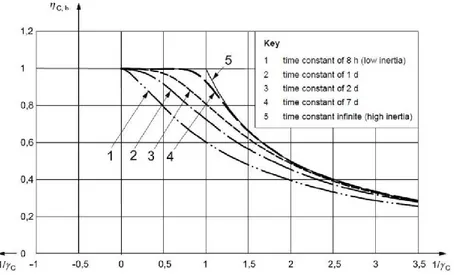
In particular, in summer conditions, the cooling load (in MJ) is given by: QC,nd= QC,gn–ƞ C,ls · QC,ht = (Qint + Qsol ) – ƞC,ls · (QC,tr + QC,ve)

Where QC,gn represents the internal load, including solar energy throughopenings, QC,ht represents the heat transfer for transmission and ventilation, ηC,lsis the loss utilization factor for cooling (non-dimensional), defined as a functionof τ and γC:

𝜂_{𝐶,𝑙𝑠} = 𝑓(𝜏, 𝛾_𝐶) where 𝜏 = C H And 𝛾_𝐶 =𝑄𝐶,𝑔𝑛 𝑄𝐶,ℎ𝑡

τ is the building time constant (h) which characterizes the inside thermalinertia of the heated space, given by the ratio between C, that is the real insidethermal capacity (J/K) and H, that it is the coefficient of thermal loss of thebuilding (W/K) (the average thermal transmittance of the building), while γC(non-dimensional) is the ratio between the free contributions by solar andinternal sources QC,gn and the total heat transfer QC,ht.

Figure 2.1 Correlation between the loss utilization factor for cooling and the gain-loss ratio

2.4 EPB Directive 2010/31/EU

In May 2010, the European Parliament approved a new legislation based on the recast of the European Directive on the energy performance of Buildings (200/91/EC). This directive aims at reducing energy consumption and greenhouse gas emissions by 20%, as well as increasing the share of renewables by 2020, in order to confront climate change, high energy prices, the growing import energy dependency and its possible geopolitical impacts (1). In fact, reduced energy consumption and an increased use of energy from renewable sources also have an important part to play in promoting security of energy supply, technological developments and in creating opportunities for employment and regional development, in particular in rural areas.

One of the key topics of the EPB Directive 2010/31/EU (formerly2002/91/EC) is the increase of the buildings energy performances insummer. A reliable assessment of the cooling consumptions (io: and interior temperature) may

beconsidered as a first useful step to understand how to improve building thermal behaviour, which depends basically on complexcorrelations between gains, losses and storage of heat.

The envelope components (i.e., walls, roofs and windows) havenot only to meet the minimum law requirements on thermalinsulation, but also have to provide a suitable thermal response tothe external heat fluxes, so that it is possible to decrease the temperaturepeaks and ensure adequate internal comfort conditions insummer. From this point of view, the estimate of the dynamic thermal propertiesof the opaque envelope components is of great importance in the thermal analysis of buildings.

As regards building performance, the impact of windows, fenestration and glazed structure is becoming more and more important, given the fact that thermal protection of opaque building elements isgradually strengthened. These structures combine many vital functions of the building (aesthetics, provision of view to the exterior, daylight thermal comfort, protection against noise, sun, cold and wind, safety, etc.) which are usually conflicting and time variant, both diurnal and seasonal. Heat transfer through windows accounts for a significant portion of the energy used in the building sector for covering both heating and cooling needs, since the optical characteristics of conventional fenestration products renders them more “vulnerable” to energy flows compared with opaque building elements.

Another international standard to take into consideration for the development of a method for calculating internal temperate in summer conditions is thestandard

UNI EN ISO 13972: 201213 792, which will be discussed later on, in the section on validation procedures.

3 The Admittance Method: a new dynamic simulation

code for building energy performance analysis.

The energy performance concerns the amount of energy consumed or estimated to satisfy all the needs of the building. As a consequence, extensive research activities, both at national and international levels, have been carried out to create a general framework for a calculation methodology of the building energy performance. Many problems have arisen, concerning the definition of energy rating, the accuracy of the calculation methodology, the discrepancies between an application to new or to existing buildings, the layout of the energy performance certificate.

In this work we have chosen to investigate and further develop the potentialities offered by Harmonic Analysis though an extension of the Admittance method. Applied to energy saving studies for buildings, the traditional method (the Admittance method proposed by the standard UNI EN ISO 13786) offers the possibility of characterizing different building components through synthetic parameters of clear physical meaning and minor computational effort. Our work aims at enhancing the traditional methodproposing a complete mathematical calculation method for the building energy evaluation.

The proposed method could serve as a sort of link between the need for simplification by the technicians (supported and endorsed by national legislation and the EU and by many international standards).

The extension of the Admittance method described by the rules and its IT development (creating user-friendly interface), would balance the needs of the technicians, focused on simplifying procedures for calculation (needs supported and endorsed by national legislation and the EU and many international standards, which allow the use of algorithms that describe the steady-state), with the need to make calculations in dynamic regime that describe the real state in much more detail, both in terms of thermal load and the evaluation of the thermal inertia and both the individual building components and inside of the building.

3.1 Decrement factor and thermal admittance

Let us consider an homogeneous slab of finite thickness, excited by sinusoidal temperature variations θsi and θso on its internal and external surface, respectively. In particular, let θ and _si θ be the mean values, whereas _so θ and _si θ are the _so respective cyclic fluctuations about the mean value.

Under the hypothesis of unidirectional conductive heat transfer through the slab in the direction normal to its surfaces, the cyclic heat fluxes _qi and _qo occurring on the two surfaces of the slab can be written as a function of the surface temperatures in the following form:

11 12 21 22 si so i o z z θ θ z z q q                  (1)

In equation (1), the heat flux qi is positive when it enters the slab surface. The elements of the transfer matrix are calculated as follows (Davies, 1994):













 





In equations (2) to (4), i is the imaginary unit (i2 _{= -1). Only two parameters} appear in the definition of the transmission matrix, namely the cyclic thickness t and the thermal effusivityξ, defined in equations (5) and (6), that collect all the data concerning the thermal properties of the material, the slab thickness L and the period P of the cyclic heat transfer:

1 2 1 2 2 2 ( ) 3600     _{ }  _   _       ω π ρc t L L λ ρc P λ (5) 1 2 2 3600       _ π λ ρ c_ _ ξ P (6)

However, in practical applications it is more useful to provide an equation that involves the air temperatures θ and _i θ instead of the temperature on the wall _o surfaces; this leads to the introduction of the surface thermal resistances Rsi and Rso.

Furthermore, it seems more suitable to consider explicitly in equation (1) the heat flux released from the wall to the indoor environment, and to hold it positive; this implies to put a minus sign before the term _qi appearing in equation (1). The final

expression for a multi-layered construction made up of n different homogenous layers becomes: 11 12 11 12 11 12 21 22 1 21 22 21 22 TRANSFER MATRIX 1 1 ... 0 1 0 1 si so i o o i n o o z z z z Z Z R R θ θ θ z z z z Z Z q q q                 _                             (7)

The transfer matrix of the multi-layered wall is obtained through the product of the matrices related to each layer, also including the matrix associated to the surface thermal resistances. In equation (7), the sol-air temperature can be used in place of the outdoor temperature when the effect of the solar radiation absorbed on the outer surface of the wall has to be taken into account.

Now, starting from equation (7), with a little algebra and taking into account the property reported in equation (8), one can calculate the heat flux released from the inner surface to the indoor environment according to equation (9):

  



It is now possible to introduce the so-called periodic thermal transmittanceX, defined as the cyclic heat flux released from the inner surface of the wall per unit cyclic temperature variation imposed on the other side of the wall, while holding a constant indoor temperature (

θ



0

12 0 1 i o θi q X Z θ _   (10)

Note that the periodic thermal transmittance resulting from equation (10) is a complex number. The decrement factorf is the amplitude of X, normalized with respect to the steady thermal transmittance U; on the other hand, the time lag φX is the phase of X, measured in hours and referred to an excitation having a period P:

X f U 

 

 

Furthermore, starting from equation (9) the thermal admittanceYcan also be introduced. This is defined as the cyclic heat flux entering the inner surface of the wall per unit cyclic temperature variation imposed on the same side, while holding a constant outer temperature (

θ



0

22 12 0 i i θo q Z Y Z θ _    (12)

However, when dealing with internal partitions separating two spaces with identical thermal conditions (

θ θ



22 12 1 i i Z q θ Z     (13)

The term (Z22 – 1)/Z12 occurring in equation (13) is called by some authors modified thermal admittance (Millbank and Harrington-Lynn, 1974), and is also referred to in the standard ISO 13792:2012.

Now, the dynamic thermal properties defined so far are usually calculated with reference to sinusoidal forcing conditions with a period P = P1 = 24 h. However,

all the relations previously introduced can also be applied to any harmonic of order n, i.e. having a period Pn = P1/n.

3.2 The surface factor

Despite the interest shown in the scientific literature towards the dynamic transfer properties, little reference is made to the thermal response of the opaque components to the radiant heat fluxes occurring on their internal surface, such as those associated to solar heat gains through the windows or to internal radiant loads.

Some attempts were done in the past in this sense. For instance, the thermal storage factor defined in the Carrier method (Carrier, 1962) is worth mentioning as the ratio of the rate of instantaneous cooling load to the rate of solar heat gain. This factor has to be determined through appropriate tables depending on the weight per unit floor area of the opaque components and the running time. Therefore, its use requires interpolation among table data, it is rather rough because it doesn’t account for the actual sequence of the wall layers, and it lacks of any theoretical basis, as it comes out from numerical simulations.

A substantially different approach can be found in the framework of the Admittance Procedure, laid down in the early Seventies (Millbank et al, 1974), where these contributions are taken into account by means of the so called surface factor. Nonetheless, the surface factor has been paid little attention: to the authors’ knowledge, little reference is made to this parameter in the whole scientific literature (Beattie and Ward, 1999) (Rees et al., 2000), while its definition has

only recently been recovered in the CIBSE guide (CIBSE, 2006) and in international Standard ISO 13792:2012.

According to the definition provided by Millbank and Harrington-Lynn (1974), the surface factor F quantifies the thermal flux released by a wall to the environmental point per unit heat gain impinging on its internal surface, when the air temperatures on both sides of the wall are held equal.

Figure 3.1 - Energy balance on the internal surface for the definition of the surface factor

With reference to Figure 3.1, let  be the cyclic radiant heat flux acting on the inner surface of the wall, as a result of the radiant energy released by internal sources or transmitted through the glazing. The following definition holds:

i o i i abs q q F q _{ }      (14) Zso Zsi



q

q

θ

θ

θ

In order to provide an operational formulation to F, one can consider that the amount of thermal energy absorbed by the wall (  ) is re-emitted to the internal and to the external environment, according to the following balance equation:

  q_i q_o

  (15)

The cyclic heat fluxes q and _i q can be written as a function of the thermal _o impedances Zsi and Zso represented in Figure 3.1:

  si i i si q Z   (16)      si o si o o so si q Z Z Z     ₍₁₇₎

In equation (16) and (17), θ_si is the temperature fluctuation measured on the inner surface of the wall. Under the hypothesis subtended in the definition of the surface factor, i.e. θ_i θ_o, it is possible to eliminate θ_si by combining equation (16) and (17): i o i si o si q Z Z Z q _{ }   (18)

Equation (18) suggests that the ratio of the heat fluxes released by the internal surface respectively to the indoor and the outdoor environment equals the inverse ratio of the corresponding thermal impedances. Now, by combining equation (18) and equation (15), one obtains:

1 i o si si i Z Z Z q Z Z              _{ }   _{ }     (19)

At this stage, one must considerthat the thermalimpedanceZsibetween the surface of the wall and the indoor air is purely resistive, thus Zsi = Rsi. Moreover, the inverse of the wall thermal impedance Z corresponds to its thermal admittance Y. Such positions imply the following expression for the surface factor F :

1 i o i si q F Y R     _      (20)

For internal partitions separating two spaces with identical thermal conditions, in equation (20) the admittance Y should be replaced by the modified thermal admittance introduced in equation (13) (Millbank and Harrington-Lynn, 1974). The value calculated according to equation (20) is a complex number, characterized in terms of amplitude |F| and phase F. The latter can be assessed through equation (21), and will always result negative, denoting a delay of the wall response to the radiant heat flux acting on it.

 

 

Hence, the surface factor depends not only on the geometrical and thermo-physical properties of the wall, but also on the period P of the cyclic radiant flux. Since in a real building any energy input linked to weather conditions can be considered periodic with a 24-hour frequency, the surface factor is conventionally calculated for P = 24 h.

Moreover, the definition of surface factor provided in equation (20) can also be applied to a steady radiant flux. In this case, the admittance Y has to be replaced by the stationary thermal transmittance U of the wall:

0 1 i o i si abs q F U R q _{  }     (22)

As to the internal surface resistance Rsi, important remarks will be given later.

3.3 The Surface Factor for monolayer walls

A first analysis concerning the behaviour of walls as a result of incident radiative fluxes can be conducted by determining the module and the phase of surface factor Z for homogeneous walls consisting of a single layer of various construction materials, to vary the layer thickness. Table 3.1 shows the thermo-physical properties of the most common building materials; in Figure 3.2 the module and the Z phase are plotted as a function of wall thickness2_{. For the} calculation of Z, the internal and external threshold resistance have respectively been assigned the following values:

Ri = 0.22 [m2_·K1_·W-1_{] Re = 0.075 [m}2_·K1_·W-1_]

These values are in fact found to be more suitable for a calculation scheme in summer rather than the standard values reported in [18] (Ri = 0.13 m2_·K1_·W-1_{, Re}

2 _{The phase of this parameter is always negative, since thermal energy is returned from the wall}

with a delay in respect to the action of the solar radiation on it; here we prefer to represent it as positive, defining it as "delay".

= 0.04 m2_·K1_·W-1_{), used for the calculation of the transmittance of the walls in} winter conditions during the project.

From the diagrams in Figure 3.2 it can be firstly noted that the curves are spaced apart in proportion to the generalized thermal effusivity, defined by:

2 c P



   (9)

For all the materials taken into consideration, a thickness of about 15 cm marks the maximum delay, more than 2.5 hours for high values of  (heavy and not very insulating material), about 1.5 hours for the average values of(light material) and less than half an hour for the insulation. In light of the results, the insulating materials appear more capable of "reflecting" the heat wave, the other vice versa in inverse relationship to the effusivity.

It is observed that, whereas the delay is reduced to zero when the thickness tends to zero, the admittance Y formally reduces to a constant value that only depends on the surface resistance, for which we have:

1 0 254    i i e R Z . R R (10)

Material Conductivity λ (W·m-1_·K-1₎ Density (kg·m-3₎ Specific heat c (J·kg-1_·K-1₎ Effusivity  (W·m-2_·K-1₎ A

Concrete with closed structure with natural

aggregates

1.16 2000 880 12.18

B Concrete with closed

structure of expanded clays 0.5 1400 880 6.69

C Autoclaved concrete 0.19 600 1010 2.89 D Hollowbrick 0.35 750 840 4.00 E Porousbrick 0.17 630 840 2.56 F Perforatedbrick 0.43 1200 840 5.61 G Solid brick 0.72 1800 840 8.90 H Blocks of tufa 0.7 1600 840 8.27 I Lava 2.9 2200 840 19.74 L Blocks of limestone 1.5 1900 840 13.20 M Polystyrene 0.036 30 1400 0.34 N Polyurethane 0.032 40 1450 0.37 O Fiberglass 0.04 35 1030 0.32 P Cork 0.045 115 1800 0.82

Q Plaster of lime and gypsum 0.7 1400 840 7.74

R Mortar of lime and cement 0.9 1800 840 9.95

S Granite 3.2 2500 840 22.11

T Marble 3 2700 840 22.24

U Timber(fir) 0.12 450 2700 3.26

V TImber (oak) 0.22 850 2700 6.06

Figure3.2 - module and delay of Z for walls monolayer according to the thickness 0 0.1 0.2 0.3 0.4 0.5 0.6 0.7 0.8 0.9 1 0 5 10 15 20 25 30 35 40 M o du lo [-] Spessore [cm]

Polistirene Porizzato Laterizio Calcestruzzo Pietra lavica

 = 0.34  = 2.56  = 4.00  = 19.74  = 12.18 0 0.4 0.8 1.2 1.6 2 2.4 2.8 3.2 0 5 10 15 20 25 30 35 40 R it ar d o [h ] Spessore [cm]

Polistirene Porizzato Laterizio Calcestruzzo Pietra lavica

 = 0.34  = 2.56  = 4.00  = 12.18  = 19.74 4.00

The conductive thermal resistance Rλ and air thermal capacity C, are respectively defined as:  _ s R [m2_·K·W-1_]    p C c s [J·m-2_{· K}-1_{] (11)}

Plotting the values of Z for every recurrent given material in Table 3.1 as a function of the previously given characteristic quantities, it is possible to construct the maps shown in Figure 3.3, valid for single-layer walls of s = 10 cm thickness. The properties of the same materials in thicknesses more usual in practice are shown in Figure 3.4.

Figure3.1 - module and delay of Z for monolayer walls - thicness s=10 cm. A B S A B C D E G H I M Q U V

Heat capacity per unit area [kJ·m-2_·K-1_]

Cond u ctive re sis tance [K· m 2 ·W -1 ] N O P

Module of Z

Heat capacity per unit area [kJ·m-2_·K -1_] Cond u ctive re sis tance [K· m 2 ·W -1 ] S A B C D E G H I M Q U V N O P

Delay in Z

B

Figure3.2 - module and delay of Z for monolayer walls - thickness given in table.

A S,T A B C D E G H I M Q,R U V

Heat capacity per unit area [kJ·m-2_·K-1_]

Cond u ctive re sis tance [K· m 2 ·W -1 ] Thickness used: A, B, F: 20 cm C, U, V: 10 cm D, G: 12 cm E: 30 cm H, I, L: 60 cm M,N: 6 cm O, P: 6 cm Q, R: 2 cm S, T: 3 cm N O P

Module of Z

Heat capacity per unit area [kJ·m-2_·K-1_]

Cond u ctive re sis tance [K· m 2 ·W -1 ] Thickness used: A, B, F: 20 cm C, U, V: 10 cm D, G: 12 cm E: 30 cm H, I, L: 60 cm M,N: 6 cm O, P: 6 cm Q, R: 2 cm S, T: 3 cm N O P

Delay of Z

3.4 The role of harmonics in the determination of Z

As mentioned above, the factor of the surface of a wall, as a dynamic parameter, depends on the pulsation of the forcing function. Solar radiation Isol can be considered, for the purpose of dynamic analysis of buildings, forcing a periodic of period P = 24 h; as such, it is possible to approximate it with an endless series of simple sinusoidal functions (Fourier series) called "harmonics". The first, frequency f1=2π / P, is called the "fundamental harmonic"; successive harmonics have frequencies equal to an integer multiple of the fundamental frequency fn=2/(P/n). We therefore have:

 

 



 

Here the term Im expresses the average value of the function Isol (τ):

 



An e Bnare the coefficients of the n-ma harmonic, given by:

 

 





In practice, the function Isol (τ) can be approximated by a series expansion that only includes an appropriate number N of harmonics, that is:

 





The accuracy in the approximation of the original function obviously depends on the number N of harmonics considered.

The surface factor Z, calculated according to Eq. (8) as provided by the standard UNI EN ISO 13792: 2005, refers to a period P = 24 h, and is therefore representative of the response of a wall solely to the first harmonic of the forcing function. In the following we will therefore try to show how this parameter is really able to describe the behaviour of the wall in respect to the periodic forcing function considered in its entirety.

First, it is interesting to highlight the extent of the contribution of each harmonic in the development in series in equation (16). The forcing function, considered here as an example, is the intensity of solar radiation that penetrates the environment through a glazed surface free of obstructions and exposed to the west; its time course is shown in Figure 3.5, together with the curves obtained using Eq. (16) to vary the number of harmonics included in the summation. The diagram shows that by restricting ourselves to the first 5 harmonics, it is possible to reconstruct the time profile of the force in question in an extremely precise way. This result can also be understood in the light of the right-hand diagram; here the effective value of Vn of each harmonic means is shown - defined as in equation (17) and representative of its energy content - normalized in respect to the effective value V1 of the first harmonic. It is clear that the weight of the harmonics decreases rapidly, becoming negligible for n>5; in any case, the

first harmonic is not sufficient to fully characterize the forcing function that acts on the wall.

 



Figure3.3 – harmonic contribution to the construction of the periodic forcing.

In the light of what we have seen so far, it is possible to write the heat flux q () emitted by a wall in response to the incident solar radiation in the following form:

 







Figure 3.5 shows the trend of module and the Z phase to vary the index of the harmonic n, for monolayer walls in different materials but of constant thickness (s = 10 cm). As can be seen, apart from polystyrene, for which the Z module is almost unitary, for all the other materials Z decreases significantly with n: the materials namely allow themselves to be more easily permeated by the thermal wave the higher the frequency, thereby reducing the rate of energy returned to the environment. The phase shift - especially for heavier materials - also shows a significant reduction in the growth of the index n of the harmonic.

0 10 20 30 40 50 60 70 80 90 100 1 2 3 4 5 6 7 8 Vn / V1 [% ] n [-]

Figure 3.6 – Dependence of Z index of the harmonic (s = 10 cm) 0 0.1 0.2 0.3 0.4 0.5 0.6 0.7 0.8 0.9 1 1 2 3 4 5 Mo d u lo [ -] N. armonica [-]

Polistirene Porizzato Forati Calcestruzzo Pietra lavica

0 0.4 0.8 1.2 1.6 2 2.4 2.8 1 2 3 4 5 Fa se [h ] N. armonica [-]

Polistirene Porizzato Forati Calcestruzzo Pietra lavica

Whereas Figure 3.6 shows the response of the walls to the solar forcing function (force) calculated according to (18), that is, by summing up the responses due to individual harmonics in which the forcing function has been decomposed. From an analysis of the curves in the figure, you can determine the actual values of attenuation and phase shift θ of the response in respect to the forcing function; in particular, the attenuation may be defined as the ratio between the peak value of the response (qmax) and the peak value of the driving force (Isol_max) and phase shift as the temporal distance between the two peaks (delay).

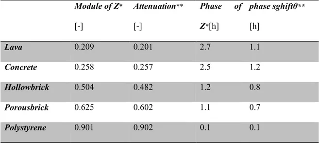
At this point, it is useful to compare the values of attenuation and phase shift so defined, with the module and the phase of the surface factor Z of the fundamental harmonic (N = 1), Table 3.2.

Note that the data of "attenuation" is very close to the “Z module”, and consequently it is only in the first harmonic that it is possible to realistically estimate the breakdown that the peak of radiation undergoes when it re-emerges from the wall as a response stream. However, the time lag between forcing function and response calculated with only the first harmonic ("Z phase") overestimates the real delay with which the absorbed solar radiation is re-emitted into the environment, and expressed in the data of "phase displacement".

The advantage of comparison comes from the fact that the regulations usually only refer to only the first harmonic. UNI EN ISO 13792: 2005, for example, in defining the surface factor, requires us to work solely with P = 24 hours, neglecting the consideration of harmonics after the first.

As shown here, therefore, makes it clear that to realistically assess the response of the system (and, by construction materials, especially the phase shift), it is not

sufficient to refer to the fundamental harmonic, but it is necessary to consider the contribution of a suitably large number of harmonics.

Figure 3.8 – Response of single-layer walls to solar forcing rebuiltwith N=5 harmonics.

Module of Z* [-] Attenuation** [-] Phase of Z*[h] phase sghiftθ** [h] Lava 0.209 0.201 2.7 1.1 Concrete 0.258 0.257 2.5 1.2 Hollowbrick 0.504 0.482 1.2 0.8 Porousbrick 0.625 0.602 1.1 0.7 Polystyrene 0.901 0.902 0.1 0.1

* : calculated for the fundamental harmonic (N = 1) ** :calculated for N=5 harmonic

Table 3.2 - Evaluation of phase shift and attenuation of the response (10 cm thick).

0 50 100 150 200 250 300 350 400 450 500 0 2 4 6 8 10 12 14 16 18 20 22 24 Fl u ss o t er mi co [W ·m -2] Tempo [h]

Forzante Pietra lavica Laterizio forato Polistirene

sfasamento θ

Isol_max

3.5 The wall energy balance

According to the definition of the previously mentioned dynamic thermal properties, it is possible to state right away the energy balance for an opaque component subject to periodic forcing conditions, while the analytical procedure for the calculation of the time-dependent internal air temperature in an enclosed spacewill be presented in the followingsection.

First of all, it is necessary to consider that the heat flux qi reported in equation (19) is the overall heat flux released by a wall per unit radiant heat flux impinging on its inner surface, where the convective and radiant terms are still combined together. However, it is important to extract the convective component of this overall heat flux, since it is the one involved in the energy balance equation of the whole enclosure.

In order to single out the convective component, one can observe that the convective and the overall heat flux are inversely proportional to the respective surface thermal resistance. Hence, equation (23) can be stated:

, ( ) ( ) i o c i c c si c r h q F h R F h h    _           (23)

Here, hc and hr are the surface heat transfer coefficients by convection and radiation, respectively. Their sum is the combined heat transfer coefficient, whose reciprocal is the surface thermal resistance, Rsi = 1/(hc + hr).

Now, equation (24) can be stated. It represents the overall density of heat flux released by a wall to the indoor environment as a response to the n-th harmonic component of the whole set of forcing conditions. Here, θo is the air temperature

on the outer side of the wall; however, it can also be interpreted as the sol-air temperature when one wants to account for both the outdoor temperature and the solar irradiation absorbed on the outer surface. On the other hand, equation (25) is the stationary term, obtained by considering the average value of each forcing condition.

Finally, the time-dependent response of the wall is obtained by recombining such contributions as in equation (26); the summation of the harmonics is truncated to the harmonic of order NH.

, , , ( ) i n n o n n i n c si n n q  X   Y   h R F     (24)







The following point to address is the determination of the radiant heat flux  circulating into the enclosure and acting on the inner surface of a wall. This term appears in equation (25) (mean value) and equation (24) (cyclic variation around the mean value), and is basically due to the solar radiation transmitted through the glazing and to the radiant component of other internal sources (lighting, appliances, people). However, its evaluation is not easy, as it implies the knowledge of the radiation distribution within the indoor environment.

In this study, the authors adopted a simplified approach, based on the Ulbricht sphere model, i.e. the hypothesis of uniform distribution of the radiant heat gains

all over the surfaces of the enclosed space. According to this model, the radiant heat flux acting on the generic surface can be calculated as:

, , 1 1 1 lw sw tot m lw m sw A r r     _  _      (27)

Here, rm is the weighted mean reflectivity of the enclosing surface, defined as:

surf surf

m k k k

k k

r  r A  A







Moreover, a distinction is made between short-wave (sw) and long-wave (lw) radiant heat gains, as the reflectivity of walls and glazing to such contributions is not the same. In equation (27) sw relates to the solar radiation transmitted through the glazing, whereas lw accounts for internal radiant sources and for the fraction of solar energy absorbed by the glazing and re-emitted towards the indoor environment. All of the data needed in equation (27) are usually known.

3.6 The room energy balance

Finally, the energy balance on the indoor environment can be written as in equation (29). Here, one can recognize the contributions due to:

(1) convective heat flux released by the opaque components, calculated according to equation (24) to (26);

(2) heat transfer through the window, that is proportional to the thermal transmittance Uw;

(3) infiltration of outdoor air, measured by the air changes per hour na ; (4) convective fraction of the internal loads, Qint (people, lighting,

appliances);

(5) convective thermal power released by heating or cooling plants.









Due to the negligible heat capacity of the indoor air, the thermal balance assumes the same form as for steady state conditions. If one needs to solve equation (29) in relation to a free-running space, Qsys () = 0.

Now, under the assumption of periodic driving forces, in equation (29) every time-dependent variable can be written as the sum of its mean value plus a series of harmonic components. Thus, the following relationship holds for the indoor air temperature θi (): , 1 ( ) H ( ) N i i i n n        



Finally, it is useful to remind that every harmonic function should comply the condition expressed in equation (31):

24/ , 1 ( ) 0 n i n     



According to these specifications, if one aims to determine the indoor temperature profile θi() for a free running space, equation (29) has to be solved in search for the following data:

 the mean value, _i;

 the harmonic components  , for n ranging from 1 to NH; _{i n,}

Thus, for every time step , a number (NH + 1) of unknown variables should be determined. This can be done since an equivalent number of equations is available.

On the other hand, for rooms under thermostat constraint, the temperature profile θi() is known a priori. In this case, equation (29) provides the dynamic thermal load Qsys ().

It is to be reminded that, despite the calculation of the dynamic thermal properties is well established in the literature, a general model based on them and aimed at finding the room thermal response, is not yet covered in the literature. Moreover, some peculiar features are introduced in the present study:

 the calculation of the surface factor with more appropriate values of the surface thermal resistance Rsi;

 the adoption of the Ulbricht hypothesis for evaluating the distribution of the radiant heat gains in the enclosed space.

Finally, it is necessary to remark that the proposed methodology, in its present form, is not suitable in case of variable parameters, e.g. with a variable ventilation rate. Indeed, in this case the variable parameter should also undergo the Fourier analysis in order to be decomposed in harmonic components, which would considerably complicate the solution of equation (29). However, an improved and more general version of the methodology is being developed at the moment.

In the following, the validation of the formulation presented so far is discussed. It is based on the procedure reported in the ISO Standard 13792, devoted to the calculation of the internal temperature of a room in summer without mechanical cooling. Furthermore, the approximation introduced by considering only the first harmonic (P = 24 h), as suggested by the simplified approach proposed in the ISO Standard 13792:2012, will be discussed.

4 The validation procedure

The validation of new mathematical codes for the dynamic thermal simulation of buildings can be performed by comparison with appropriate reference values, obtained through experimental measurements or by means of well established codes.

In particular, the international Standard ISO 13792 proposes a procedure that allows the validation of mathematical models for the calculation of the summer internal temperature in enclosures without mechanical cooling. The procedure consists in the calculation of the hourly profile of the operative temperature for a test room in different conditions; for every test case, the minimum, average and maximum values of the operative temperature shall then be compared to the reference values reported in the Standard. As far as its reliability is concerned, the computer code under examination will belong to class I, II or III based on the difference Δ between the calculated values and the reference values; the model is classified according to the worst result:

 Class I: -1°C << 1°C

 Class II: -1°C << 2°C  Class III: -1°C << 3°C

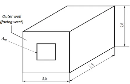
Figure 4.1 reports the geometry of the test room. Two different cases are considered: in Case A the surface of the window is Aw = 3.5 m2_{, whereas Aw = 7.0} m2 _{in case B. The climatic conditions are also different (see Figure 4.2): case A}

applies to warm climates (latitude 40°N), whereas case B applies to temperate climates (latitude 52°N).

For each room geometry, different sub-cases are considered, distinguished by a test number (from 1 to 3, according to the type of floor/ceiling) and by a second letter, associated to the ventilation rate (case a: 1 h-1_{, case c: 10 h}-1_{). There is also} a sub-case b, that applies to a variable ventilation rate, but this is not considered in the framework of this study, since the proposed model only allows constant parameters.

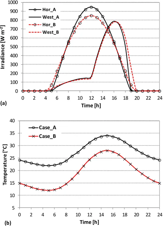
Figure 4.2 - Climatic data for the validation. (a) Solar irradiance, (b) Outdoor temperature

As concerns the composition of the opaque components, the external wall is made up of a double layer of masonry (115 mm plus 175 mm) with an intermediate insulation layer (60 mm) and an internal plastering (15 mm). The partition walls consist of two gypsum wallboards (12 mm each) with an intermediate layer of

0 100 200 300 400 500 600 700 800 900 1000 0 2 4 6 8 10 12 14 16 18 20 22 24 Ir ra d ia n ce [W m -2 ] Time [h] Hor_A West_A Hor_B West_B (a) 5 10 15 20 25 30 35 40 0 2 4 6 8 10 12 14 16 18 20 22 24 Temp er a tu re [° C] Time [h] Case_A Case_B (b)

mineral wool (100 mm). Ceilings and floors are basically composed of a concrete slab (200 mm) covered with an insulation layer (40 mm) plus a concrete screed (60 mm). In the test number 1, a further insulation layer (100 mm) is added to the bottom of the concrete slab. All the surfaces, except the outer wall and the roof in the test number 3, are bounded by similar rooms. The short-wave surface absorptance is  = 0.6.

Now, in the calculation of the dynamic thermal properties (X, Y and F), the ISO Standard 13792 prescribes to use Rsi = 0.22 m2 _{K W}-1 _{for any surface. However,} in this study such recommended value has been used only for the calculation of X and Y. Instead, the surface factor F is calculated through more appropriate values, introduced in Evola and Marletta (2013) and reported in Table 4.1, together with the recommended values for the convective heat transfer coefficient hc to be used in equation (23).

Walls Ceiling Floor

Rsi [m2 K W-1] 0.6 0.85 0.7

hc [W m-2 K-1] 1.4 1.0 1.2

Tabella 4.1 Values retained for Rsi and hc in the calculation of the surface factor

Table 4.2 collects the dynamic thermal properties for the vertical and horizontal envelope components, calculated for the fundamental harmonic (P = 24 h) with the relations introduced in the previous sections.

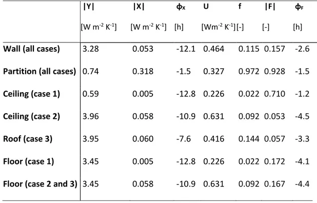
From Table 4.2 one can learn that the opaque components that contain an insulation layer very close to the internal surface, i.e. the partitions and the ceiling

in test case 1, show a surface factor F quite high and a low time shift F. This means that these envelope components tend to give back a very high portion of the radiant heat flux absorbed on their inner surface, and this happens within around one hour. On the contrary, all other components allow a significant attenuation of the radiant heat flux acting on their inner surface (low |F|), with a rather high time lag F.

Table 4.2 - Dynamic thermal properties for the room components defined in ISO 13792:2012 (in brackets, the test cases)

|Y| |X| φX U f |F| φF

[W m-2 _K-1_{] [W m}-2 _K-1_{] [h] [Wm}-2 _K-1_{][-] [-] [h]}

Wall (all cases) 3.28 0.053 -12.1 0.464 0.115 0.157 -2.6 Partition (all cases) 0.74 0.318 -1.5 0.327 0.972 0.928 -1.5 Ceiling (case 1) 0.59 0.005 -12.8 0.226 0.022 0.710 -1.2 Ceiling (case 2) 3.96 0.058 -10.9 0.631 0.092 0.053 -4.5 Roof (case 3) 3.95 0.060 -7.6 0.416 0.144 0.057 -3.3 Floor (case 1) 3.45 0.005 -12.8 0.226 0.022 0.172 -4.1 Floor (case 2 and 3) 3.45 0.058 -10.9 0.631 0.092 0.167 -4.4

As concerns the window, it is composed by a double pane glazing with an external shading device. The external, internal and cavity thermal resistances are assigned: as a results, the thermal transmittance Uw is 2.2 W m-2 _K-1_{. Furthermore,}

the short-wave optical properties of both the glazing and the shade are assigned: this allows to easily calculate the rate of solar irradiance transmitted through the window, or absorbed by the glazing and re-emitted towards the indoor environment.

Finally, the ISO Standard also prescribes the time profile of the internal sources to be used in the simulations (people, appliances), and assigns an equal proportion to convection and radiation (xc = 0.5).

Thus, all the input values needed for the simulations are assigned, and they can be easily implemented in the calculation procedure. The calculation is carried out by using NH = 6 harmonics, since a preliminary analysis showed that no significant improvement of the results would be achieved by adding further harmonics. As a result, the time profile of the indoor temperature θiis obtained. This result can be also used to determine the mean radiant temperature θmr, according to equation (32):









This derives from the position that, if all the inner surfaces present the same temperature θmr, no reciprocal radiant heat exchange would occur, but only a convective heat transfer to the indoor air. Finally, the room operative temperature is provided by equation (33). ( ) ( ) ( ) 2 mr i op         (33)

5 Validation of the proposed model

As described before, several test cases are considered in ISO Standard 13792. In particular, the test cases are aimed to check the reliability of the proposed model as follows:

 in relation to the size of the window and the climatic data (Case A or Case B);

 in relation to the features of the envelope components (Case 1, Case 2, Case 3);

 in relation to the rate of infiltration from outdoors (Case a or Case c). The combination of these features produces a total of 12 different cases.

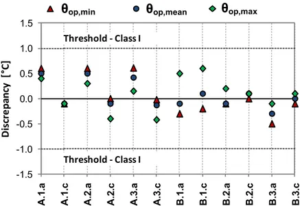
Now, Figure 5.1 shows the discrepancy Δ between the value of the room operative temperature calculated through the proposed methodology, and the reference values provided in the ISO Standard, for each test case considered in this study. The compliance of the calculation procedure to the Standard has to be assessed by looking at the minimum, the average and the maximum room operative temperature; thus, the diagram reports the discrepancy for each one of these parameters.

In Figure 5.1 there is also an indication of the threshold discrepancy in order for the calculation procedure to be rated in Class 1 (-1°C < Δ < 1°C). According to the displayed results, it is possible to state that the proposed methodology has a good reliability in the determination of the indoor operative temperature in free-running enclosures. Actually, not only the methodology can be classified in Class

I, but the discrepancy measured over the whole set of test cases is within ± 0.6°C. As a general rule, the best results pertain to the simulations characterized by high infiltration rates (na = 10 h-1_{, cases c).}

Figure 5.1 - Compliance of the proposed methodology with the ISO Standard

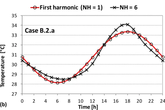
5.1 The effect of higher order harmonics

In the previousparagraph, it is shown that the analytical methodology presented proves sufficiently reliable with NH = 6 harmonics. However, one must remark that both in the scientific literature and in the international Standards the dynamic thermal properties are normally used by looking only at the fundamental harmonic (n = 1).

Now, with reference to the cases A.2.a and B.2.a, Figure 5.2 shows that the room operative temperature calculated with NH = 1 is not very different from that obtained with NH = 6. Indeed, the difference between the two profiles does not

-1.5 -1.0 -0.5 0.0 0.5 1.0 1.5 A .1 .a A .1 .c A .2 .a A .2 .c A .3 .a A .3 .c B .1 .a B .1 .c B .2 .a B .2 .c B .3 .a B .3 .c D is cre p an cy [ °C]

Minimum Average Maximum

Threshold - Class I

Threshold - Class I