Development of a stabilized Ti:Sa frequency comb for frequency comparisons at high stability in the optical region

(1)

Universit`a degli Studi di Pisa Dipartimento di Fisica ”E.Fermi”

Tesi di Dottorato

Dottorato di Ricerca in: Fisica – Ciclo XXIII (2008)

SSD – FIS/03

Development of a stabilized Ti:Sa

frequency comb for frequency

comparisons at high stability in the

optical region

Candidato:

Denis Sutyrin

Supervisore:

Coordinatore:

Professore Nicol`

o Beverini

Professore Guglielmo M. Tino

(2)

(3)

Dedication

In memory of my Mom.

In life she was my best friend, and in death she is always

motivating me to live and to work

(4)

(5)

Acknowledgments

There are so many people that have helped me in so many ways. I could never name all those that contributed to my thesis and my life in ways both large and small. However I will take this small space and do what I can to acknowledge at least a few.

I could not have produced this thesis without the help of a very long list of people both inside Florence University-LENS, Pisa University and out, where they helped me along my professional and personal journeys. The list is, of course, too long to remember to thank everyone, but here is where I shall try. I am extremely grateful to each of them.

First of all, I would like to thank a lot my supervisor Prof. Nicolò Beverini. Despite on that I did my PhD about 80 km far from his office, I always feel his scientific and mental support to work on the thesis. I thank to Prof. Guglielmo Tino, who gave me the opportunity to work in his perfect laboratory with so many intelligent and friendly people.

The special thanks goes to Dr. Nicola Poli. We worked side-by-side for most of the construction and subsequent experiments, and I have come to admire his patience and generosity. I am a much better scientist because of his tutelage, and for that he has my gratitude.

My thanks to Dr. Sergei Chepurov, from whom I learn a lot about nature and femtosecond comb development. His ideas and recommendations were ex-tremely helpful during all my work. I really happy to meet during the Prof. Marco Prevedelli, who is expressive example of accuracy and precision in work for me.

The work presented in Appendix A was performed in the optical clock labora-tory at the Institute of Laser Physics in Novosibirsk. I am immensely grateful to people in the Novosibirsk, especially Prof. Vladimir Denisov, for making my visit possible to do science. I was privileged to work closely with Sergei Kuznetsov,

(6)

One of the main trouble for me in Italy was bureaucracy. For this reason I would like to thanks all people, who helps me to solve them, especially secretaries in Florence University, Elisa Tonelli, and in Pisa University, Ilaria Fierro.

I would like to thank all people who help me in work and also did my life in Italy more entertaining: Marco Tarallo and Marco Schioopo (for too many thing to remember), Yu-Hung Lien (you organized many of grate events), Gabriele Rossi (you always gave me something useful from you lab), Giancarlo Ferrera (too many helps plus you was inspirer of soccer matches), Andrea De Michele (we start to build it together).

(7)

Abstract

This dissertation describes the development of a self-referenced optical frequency comb (OFC) based on a Ti:Sa femtosecond (fs) laser, to be employed in frequency comparisons between a strontium optical lattice clock and other frequency refer-ences, both in the radio-frequency (RF) and in the optical domain.

The Ti:Sa mode-locked laser, which employs external ﬁber broadening (EB) for the generation of octave-spanning spectrum, has been stabilized by locking an OFC tooth to a clock laser with high spectral purity, operating at 698 nm and resonant with the clock transition 1_S

0-3P0 in neutral strontium atoms.

The frequency stability of this EB OFC has been tested both in the RF domain by comparison with a high-quality quartz oscillator slaved to the global positioning system (GPS) signal, and in the optical domain with a second stabilized diode laser at 689 nm slaved at long term to the intercombination transition1_S

0-3P1 in atomic

strontium.

We perform a frequency noise and intensity-related dynamics characterization of the free-running fs Ti:Sa EB OFC and implement these results for optimizing the phase–lock of the OFC to a Hz-wide 698 nm semiconductor laser. Based on the frequency noise of the beatnote between the clock laser and corresponding EB OFC tooth fb698 we expect that the short term frequency stability of the 698 nm

clock laser is then transferred to each tooth of the octave-spanning EB OFC. Moreover, the noise transfer processes between the pump laser and the Ti:Sa laser have been studied in detail, both comparing the resulting frequency noise of the EB OFC output spectrum with a single-mode Coherent Verdi V5 and a multi-mode Spectra Physics Millennia Xs 532 nm pump lasers. In particular, in the latter case we demonstrate that the implementation of an additional control loop for the stabilization of carrier-envelope oﬀset (CEO) frequency fCEO allowed

us to stabilize this signal at mHz level, that is compatible with fCEO stabilization

(8)

698 nm the impact of fCEO frequency noise on the frequency noise of any EB OFC

tooth is negligible when compared with the frequency noise of the fb698.

Despite the OFCs are used typically for precision frequency measurements, we demonstrate an approach to perform an absolute frequency measurement of unstable frequency by the EB OFC.

Most of this thesis is devoted to the EB OFC. However, I also present char-acteristics and our ﬁrst stabilization results of the OFC working at quasi octave-spanning (QOS) regime.

(9)

List of Figures

1.1 Harmonic optical frequency chain . . . 4

1.2 Using atomic resonances for optical mixing . . . 5

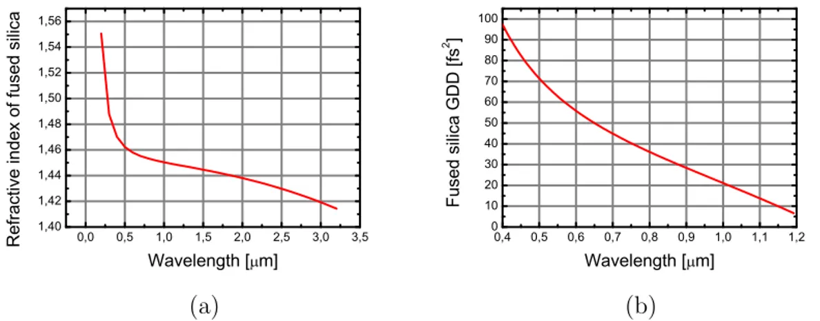
2.1 (a) Refractive index of fused silica. (b) GDD of fused silica . . . 26

2.2 Schematic diagram of a Gires-Tournois interferometer (GTI) . . . . 29

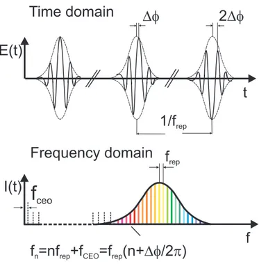
2.3 The basic time- and frequency-domain representations of the output of a mode-locked femtosecond laser . . . 34

2.4 Kerr lens mode-locking . . . 35

2.5 Two equivalent schemes for the measurement of fCEO using an

octave-spanning OFC . . . 37

2.6 Fixed point model description for diﬀerent types of ﬂuctuations in the laser . . . 45

2.7 (a) Deﬁnition of frequency terms: ω0 is the gain peak, ωcis the pulse

spectral peak, ωrms is the pulse spectral width, and ω∆ = ωc− ω0.

(b) Schematic showing the spectral shift eﬀects . . . 46

2.8 Linear relationship between dfCEO/dP and dfrep/dP with a slope of

β0/(2π) . . . 52

2.9 The measured dfrep/dP versus pump power. . . 53

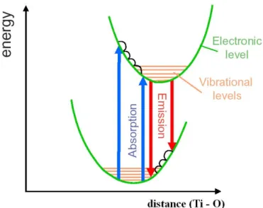
3.1 The energy levels diagram for Ti:Sa . . . 62

3.2 (a) Index of refraction for Ti:Sa plotted for Sellmeir’s equation. (b) GDD of Sapphire . . . 63

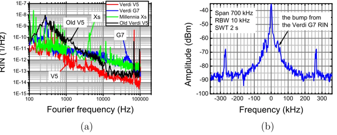
3.3 (a) The RIN of all pump lasers used to pump the OFC. b) Free-running fCEO of the OFC pumped by Verdi G7 . . . 65

3.4 Commonly used cavity for Ti:Sa laser . . . 65

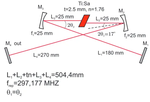
3.5 Schematics of our X folded Ti:Sa cavity . . . 66

(16)

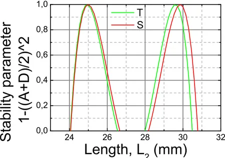
3.6 Regions for distance L2 between mirror M2 and Ti:Sa crystal when

the cavity is stable . . . 69

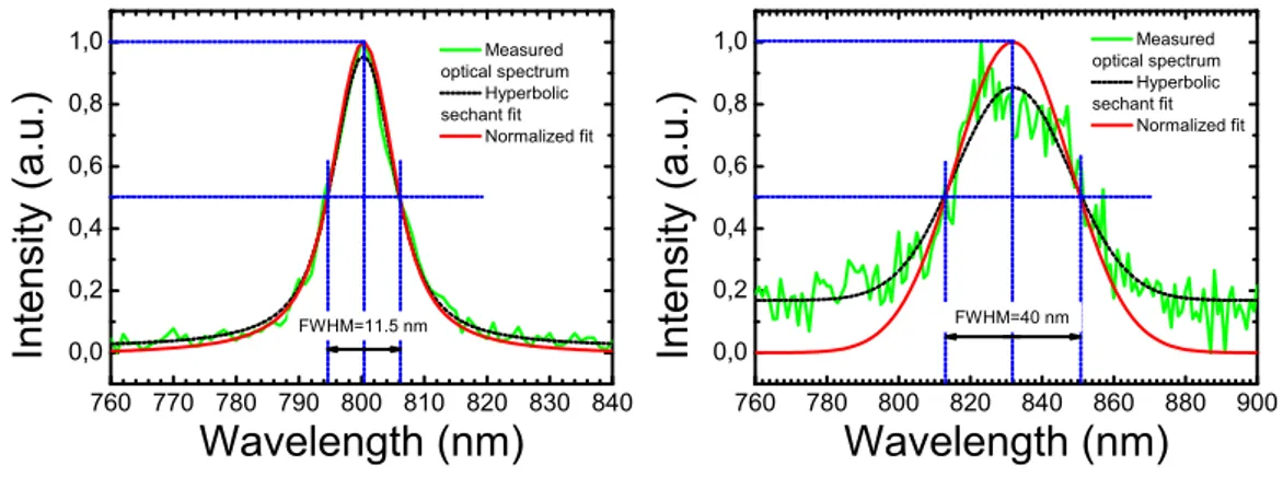
3.7 Emission optical spectrum of Ti:Sa laser in fs regime with total cavity dispersion ∼ −400fs2 _{(left) and} _{∼ −150fs}2 _{. . . .} ₇₀

3.8 The passive stability of our OFC . . . 72

3.9 (a) - Conﬁguration for using an AOM as a noise eater. (b) - Pump beam horizontal shifting . . . 74

3.10 Experimental setup of Ti:Sa OFC . . . 75

3.11 (a) - Typical measured dispersion of the ﬁber in the FEMTOWHITE 800. (b) - Principle behind the beam expansion in the device. . . . 76

3.12 Supercontinuum optical spectrum after the PCF . . . 78

3.13 Scheme for beam focusing in the BBO crystal . . . 80

3.14 (a) Scheme for beam focusing in the BBO crystal. (b) Typical observed fCEO signal . . . 80

3.15 QOS OFC cavity scheme . . . 81

3.16 (a) QOS OFC output optical spectrum at diﬀerent levels of the pump power. (b) QOS OFC broadest observed output optical spec-trum . . . 82

3.17 (a) QOS OFC output power as a function of the pump power. (b)

fCEO as a function of the pump power (case of the mml pump). . . 82

3.18 (a) frep of the free-running QOS FOC. (b) fCEO of the free-running

QOS FOC . . . 83

3.19 Experimental setup for the 698 nm clock laser frequency stabiliza-tion and characterizastabiliza-tion . . . 84

3.20 (a) Frequency noise of the stable 698 nm laser source locked to its ultra-high-ﬁnesse cavity. (b) Stability curves for the clock laser system 86

4.1 Measured intensity-related spectral shift . . . 92

4.2 Measured amplitude noise of sml and mml . . . 94

4.3 The calculated OFC tooth linewidth across the free-running OFC spectrum . . . 96

4.4 Electronics for the OFC stabilization . . . 97

4.5 Allan deviation of our local oscillator . . . 98

(17)

LIST OF FIGURES

4.6 The noise spectral densities and the relative estimated Allan

devi-ations of the phase-locked fCEO . . . 100

4.7 The noise spectral densities and the relative estimated Allan devi-ations of the phase-locked fb698 . . . 102

4.8 Relative contributions of the frequency noise of fCEO and the beat-note frequency between the OFC and the clock laser to a certain OFC tooth. . . 104

4.9 (a) Frequency noise of the stabilized fCEO and fb698 signals. (b) Frequency noise of diﬀerent teeth of our EB OFC phase-locked to the clock laser. . . 104

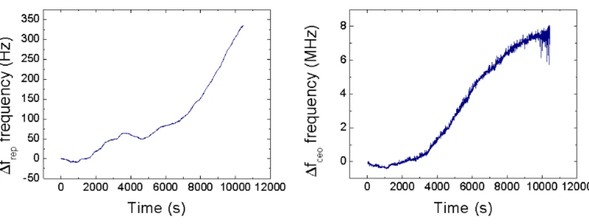
4.10 Frequency counting of fb698 (Left) and frep (Right) signals of phase-locked QOS OFC to the clock laser . . . 106

4.11 fCEO (Left) and fb698 (Right) phase noise of phase-locked QOS OFC106 4.12 (a) Allan deviation of the fCEO of the QOS OFC pumped by Verdi G7. (b) Locked fCEO signal . . . 109

5.1 Schematic view of the experimental apparatus . . . 113

5.2 The frequency measurement of the frep and fCEO . . . 114

5.3 The frequency measurement of the frep and fCEO . . . 115

5.4 (a) Beat-notes between the OFC and 689 nm laser. (b) Allan devi-ation of the optical ratio . . . 117

5.5 Beat-notes between Verdi and the OFC . . . 120

5.6 Verdi absolute frequency measurement . . . 122

A.1 The setup for PZT resonances measurement . . . 152

A.2 PZT frequency resonance . . . 152

A.3 PZT phase resonance . . . 153

C.1 689 nm laser experimental scheme . . . 160

D.1 Experimental setup for Verdi frequency calibration and 1D 88Sr op-tical lattice . . . 164

E.1 Optical setup of the wavemeter . . . 167

F.1 Oscillator Spectrum . . . 170

(18)

F.2 Phase noise, fractional-frequency noise and Allan variance . . . 175

F.3 Simpliﬁed schematic of laser feedback loop . . . 181

(19)

List of Tables

4.1 Values used in calculations . . . 107

4.2 Fixed Point, Frequency Dependence, and Magnitude of the Various Contributions to the Frequency Noise on the Comb Lines . . . 108

5.1 Rules for choosing sign of fCEO and frep frequencies . . . 114

A.1 Measured frequencies of molecular iodine . . . 154

B.1 Physical properties of Ti:Sa . . . 157

F.1 Phase noise . . . 174

(20)

(21)

Chapter 1 Introduction

The creation and application of OFCs for precision measurements are the results of investigations and developments in the ﬁeld of optical frequency measurement systems. Therefore, I would like to start describing in Sect. 1.1 the idea of the development of such systems. Sect. 1.2 describes investigations about detailed study of OFCs itself. While in Sect. 1.3 I focus on the historical results to create OFC and implement for frequency measurements.

1.1 The development of optical frequency

mea-suring systems

The invention of the laser [1] made a revolution in many ﬁelds of science: spec-troscopy, material processing, photochemistry, microscopy etc. and also in mili-tary, medicine and industry. Our interest is the laser impact on Metrology.

Heterodyne beatnotes experiments between independent lasers showed that lasers could have an excellent spectral and spatial coherence with relatively narrow linewidths, δν, and correspondingly low fractional uncertainty, δν/ν0, where ν0 is

the atomic transition frequency. The stability of frequency standard in the optical region potentially can be better than in microwave due to the fact that Allan deviation is determined as σy(τ ) = δν(τ )rms ν0 = 1 πQ √ Tc 2N0τ (1.1) 1

(22)

where δν(τ )rms is the measured frequency ﬂuctuation, Tc is the cycle time (i.e.,

the time required to make a determination of the line center), N0 is the number

of participating particles (atoms), τ is the total averaging time, Q = ∆ν/ν0 is the

resonance quality factor of an optical clock transition.

Due to its high frequency, the practical implementation of optical standard has a signiﬁcant technical challenge. This is because an absolute frequency mea-surement must be compared with the primary standard, which since 1967, is the hyperﬁne transition of a cesium atom with frequency of about 9 GHz. Optical standards have frequencies ∼50 000 times higher. There were no devices that could link directly microwave and optical regions.

At the beginning, for solving this task, the natural method was to start with the highest possible frequency from the oscillator, that can be coherently controlled and linked to the primary standard and then step by step multiply its frequency up to the optical region by using diﬀerent types of nonlinear devices.

For this approach were developed new techniques of frequency multiplication that can work from microwave to IR region. Practically, from 1960 up to 1990, this approach was realized by using klystrons or backward wave oscillators for high frequency generation (up to 300 GHz). These devices could be phase–locked to microwave standard through low-frequency microwave mixing techniques and quartz crystals. The frequency multiplication step from hundreds of GHz to IR region demanded new methods and devices. To avoid the use of too many stable oscillators to span the electromagnetic spectrum, new devices should have had the highest possible frequency multiplication factor. Moreover, they had to be able to work in the microwave and IR regions. The search of such devices give us three interesting devices: whisker-contacted Schottky diodes, point-contact Metal-Insulator-Metal (MIM) diodes and superconducting Josephson mixers [2–5].

With new nonlinear mixers was possible to reach the 2-5 THz range. Above this region it was necessary to use FIR lasers with which was possible to reach

∼30 THz. To coherently generate a visible laser frequency near 500 THz starting

from a 1 THz source and relying only on successive stages of second-harmonic generation would require 2N = 500, or N ≈ 9, stages. With judicious choices of FIR lasers and mixers it was possible to achieve higher-order mixing (e.g. ×10

or ×12) in the THz range. This meant that is was possible to jump in a single

step from a FIR laser at ∼1 THz to another FIR laser at ∼10 THz. With two

(23)

1.1 The development of optical frequency measuring systems

additional mixing orders, the 10 THz signal can be multiplied up to the 30 THz frequency of the convenient, powerful and stable CO2 lasers [6].

At frequencies above 30 THz, MIM diode mixers are suitable for some mixing and harmonic generating applications (e.g. 3× 30 THz = 90 THz), but nonlin-ear optical crystals can be very effective alternatives because they can be phase-matched for efficient mixing of specific desired frequencies/wavelengths.

Unfortunately, at higher frequencies no convenient nonlinear mixing elements were found that could generate continuous wave (CW) high harmonics. Lacking that, the mixing orders were necessarily low, and optical frequency chains required several stable laser sources spanning the frequency range and all locked together with phase-locked-loops - hence the analogy of a chain with interlocking loops. Several big labs worked on harmonic optical frequency chains that used these ap-proaches to reach important optical frequency references directly from microwave frequency sources. They continued to develop and reﬁne optical frequency mea-surement methods and synthesis chains that were used to measure and evaluate optical frequency standards [4,7–19].

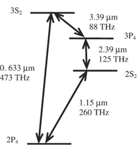
Because of their complexity and specialized applications, only a small number of optical frequency chains were ever constructed. One of such setup is presented in Fig.1.1. This was the frequency chain developed by Chebotayev’s group at Novosi-birsk and conﬁgured to operate as an optical time scale, i.e. an ‘optical clock’. The frequency chain was controlled from a CH4 frequency standard at 88 THz

(3.39 µm) at the top and delivered an output at a RF/microwave frequency [20]. A novel way around the problem of the lack of any efficient nonlinear mixers for low-power CW lasers was the concept from Klement’ev et al. [21] who proposed using resonant interactions in atoms to efficiently sum three optical frequencies to generate a fourth. Specifically, they proposed using Ne atomic resonances to sum the well-known He-Ne laser lines at 3.39 µm, 1.15 µm and 1.5 µm in order to generate the 633 nm laser line as shown in Fig.1.2. The advantage is that resonant atomic nonlinear mixing can be 8 to 10 orders of magnitude stronger than that found in bulk nonlinear optical materials. The obvious disadvantage is that the optical mixing is not broadband, and so only very specific frequencies can be generated. The four-photon optical mixing approach of Fig.1.2 was demonstrated in Russia [21] and was also used at NIST for the measurement of the 633 nm He-Ne frequency [3].

(24)

Figure 1.1: Harmonic optical frequency chain. It was developed by Chebotayev’s group at Novosibirsk and conﬁgured to operate as an optical time scale, i.e. an ”optical clock”. The yellow boxes are sources, the green boxes are phase-locked loops, the red circles are harmonic mixers.

Demonstration of optical molecular clocks were done in Novosibirsk [23] and at PTB [7]. Both used He-Ne/CH4 optical frequency standard. Optical clock on

I2 was demonstrated in [24], and on cold atoms/ions in [25–28].

Great improvements of optical clock frequency uncertainty were at the begin-ning of 2000. These were the results of optical standards referred to laser cooled

(25)

1.2 Basic principle of the optical frequency measurements using an OFC

Figure 1.2: Using atomic resonances for optical mixing. It was proposed by

Kle-ment’ev et al. [21] and ﬁrst demonstrated in USSR using the Ne transitions shown here. This scheme was also implemented by a team at NBS using 8 m long He-Ne gain tubes in a measurement of the frequency of the 473 THz (633 nm) laser [3,22].

and trapped atoms/ions and of the developments of fs OFCs. Cold atoms/ions were developed in many laboratories around the world and fs OFC technology provides practical optical synthesizers and frequency dividers.

1.2 Basic principle of the optical frequency

mea-surements using an OFC

In 1998, H¨ansch and co-workers introduced a revolutionary approach vastly

simpli-fying optical frequency measurements. By using the modes of optical frequencies emitted by a mode-locked fs laser as a ruler, they were able to measure diﬀer-ences of several tens of THz between laser frequencies [29–31]. Next several ex-periments [32–36] deﬁnitely pointed out that, by establishing a phase-coherent link between optical frequencies and the radio frequency domain, the modes of a mode-locked fs laser could be used as an extremely precise and absolute ruler in frequency space.

The emission of a mode-locked fs laser is formed by an ideal regular train of optical pulses and its optical spectrum presents a series of repeating, equally

(26)

spaced spectral lines.

The spacing of the spectral lines of such OFC is given by the repetition rate

frep at which pulses are emitted from the mode-locked laser, while the phase shift

∆ϕCEObetween the pulse carrier and the pulse envelope each round trip determines

the overall oﬀset of the comb elements fCEO = frep(∆ϕCEO/2π). The relationship

between these two parameters and the nth _{element of the OFC is given by the}

simple expression

νn= nfrep± fCEO (1.2)

where n ≈ 106_{. Here and later in the thesis, the symbol ν refers to optical}

frequencies, while f - to RF frequencies. The unknown absolute optical frequency of a cw laser, whose frequency lies close to OFC tooth n, can be determined by the equation

νcw = νn± fb = nfrep± fCEO± fb (1.3)

where fb is the beatnote between cw laser and corresponded OFC tooth n.

For a high-precision determination of fCEO, it must be directly measured, and

typically it is performed by using nonlinear frequency generation to compare dif-ferent regions of the frequency comb [37]. For example, if the laser spectrum covers more than one octave, then the OFC teeth at the low-frequency end of the spec-trum can be doubled in a nonlinear crystal and subsequently heterodyned against the high-frequency teeth of the OFC to yield fCEO. An important advance in this

respect is the generation of octave-spanning spectra with low-power Ti:Sa lasers in microstructured ﬁbers [38,39], or by direct generation from the laser itself [40–42]. Once measured, fCEO can then be locked at a ﬁxed frequency with the use of

servo-control techniques.

Phase-lock of one tooth n of the OFC can be done to the low-noise cw laser, that has itself been steered to an atomic resonance, or directly to a known microwave standard.

OFC becomes a ﬁnal tool in the long history of the development of optical frequency measuring systems. The dramatic simpliﬁcation of a complex optical frequency chain to a single mode-locked laser has facilitated optical frequency measurements. An important aspect of this new technology is its high degree of

(27)

1.3 History of OFC development

reliability and precision together with a lack of systematic errors. For example, it has been shown that the frep of a mode-locked laser equals the mode spacing to

within the measurement uncertainty of 10−16 [29]. The uniformity of the comb’s mode spacing has also been veriﬁed to a level below 10−17 [29], even after spectral broadening in ﬁbers.

OFCs are used nowadays in many applications including optical frequency metrology [36,43,44] optical clocks [45,46] comb-calibrated tunable lasers [47–49], OFC spectroscopy [50–52], frequency/time transfer [53,54], low-phase-noise mi-crowave generation [55–57], calibration of astronomical spectra [58] and search for variations of fundamental constants [59,60].

1.3 History of OFC development

Mode-locking was ﬁrst demonstrated in the mid-1960s using a He-Ne laser [61], a ruby laser [62], and a Nd:glass laser [63]. Unfortunately, from the early 1960s until about 1990, the pulsed and cw lasers communities continued to diverge. The cw lasers community worked on the stability of their lasers. While pulsed lasers researches were focused on escalation of pulsed power.

The key technique for mode-locking was Q-switching based on the implementa-tion of saturable absorbers. It was generally preferred to obtain high pulse energy rather than stability.

In the period from 1970s up to 1980s interest of researchers was focused on ultrafast dye lasers. For this type of laser Q-switching instabilities are not a problem, and also dye lasers soon allowed the generation of much shorter pulses. In 1974 the ﬁrst sub-picosecond passively mode-locked dye laser [64–66] and, in 1981, the ﬁrst sub-100-fs colliding pulse mode-locked (CPM) dye laser [67] were demonstrated.

In the 1980s begins a time when diode lasers achieve an average power high enough for pumping solid state lasers. This provides dramatic improvements in efficiency, lifetime, size, and other important laser characteristics. For example, actively mode-locked diode-pumped Nd:YAG [68] and Nd:YLF [69–72] lasers gen-erated 7-12 ps pulse durations for the first time. In comparison, flashlamp-pumped Nd:YAG and Nd:YLF lasers typically produced pulse durations of ≈100 ps and

(28)

mod-elock diode-pumped solid-state lasers resulted in Q-switching instabilities.

The ﬁrst signiﬁcant step in ultrafast solid-state lasers was performed in the end of 1980s, when was demonstrated the Ti:Sa laser [75]. The strong interest in an all-solid-state ultrafast laser technology was the driving force, and formed the basis for many new inventions and discoveries.

The next significant step in ultra-short pulse production was made in 1990. Two important papers were presented: Ishida et al. presented passively mode-locked Ti:Sa laser with an intracavity saturable absorber dye that produced stable 190 fs pulses [76]. Second, Sibbett’s group presented 60 fs pulses from a Ti:Sa laser that appeared not to have a saturable absorber [77]. This second result -in the absence of a visible saturable absorber - had an immediate impact on the research community, but the ultrafast laser experts realized that the first result was also very surprising, even though a saturable absorber was present. It was clear that the dye saturable absorber, with a recovery time in the nanosecond range, could not support ultrashort pulses with a Ti:Sa laser as it could with dye lasers. Sibbett’s modelocking approach was initially termed ‘magic modelocking’, and it triggered a major research effort into understanding passive modelocking of solid-state lasers. This form of modelocking was soon explained [78–80] and is now referred to as Kerr lens modelocking (KLM). Ishida’s result was also explained by KLM: the slow dye saturable absorber only provided a reliable starting mechanism for KLM.

The short pulses from these systems provide a very broad optical spectrum. However, it is also important also that spectrum also is stable comb-shaped, where the spacing of the individual longitudinal modes exactly equals the pulse repetition rate. Phase-locking the optical frequencies of the OFC to a laser serving as the oscillator of the clock results in the phase-locking of the OFC spacing (i.e., the laser repetition frequency) to the clock’s oscillator as well. Therefore, the OFC provides the phase-coherent division from an optical frequency to a microwave frequency, and the clock output is the repetition frequency of the mode-locked laser producing the comb.

The OFC produces a ”ruler” in the frequency domain with which an unknown optical frequency can be measured. However, many years passed before this ”sim-ple idea” [81] to use OFC was realized.

(29)

1.3.1 Bulk crystal based: Ti:Sa OFC

OFC can be produced by several types of lasers. Nowadays, three groups of OFCs can be outlined: bulk crystal based, ﬁber-based and microresonator-based OFCs. Among them, the bulk crystal based group is our interest.

The main active medium in bulk laser is Ti:Sa. The working principle of it is a Kerr-lens. The primary reason for using Ti:Sa is its enormous gain bandwidth (700-1000 nm), which is necessary for supporting ultrashort pulses as ruled by the Fourier formula. Moreover, a Ti:Sa crystal also serves as the nonlinear material for mode-locking through the optical Kerr effect which manifests itself as an increase of the nonlinear index at increasing optical intensity. Since the transverse intensity profile of the intracavity beam is Gaussian, a Gaussian index profile is created in the Ti:Sa crystal, which makes the latter equivalent to a lens. As a consequence, the beam tends to focus, the focusing increasing with the optical intensity. To-gether with a correctly positioned effective aperture, the nonlinear (Kerr) lens can act as a saturable absorber, i.e. high intensities are focused and hence are fully transmitted through the aperture, while low intensities experience losses.

Since short pulses produce higher peak powers, they experience lower losses, making mode-locked operation favorable. This mode-locking mechanism has the advantage of being essentially instantaneous, but has the disadvantages of not being self-starting and of requiring a critical misalignment from optimum cw oper-ation. Since most of the pulse broadening in ultrashort pulses is caused by group delay dispersion (GDD) of the gain medium, to obtain the shortest possible pulses from the laser cavity the overall GDD has to be near zero. To counteract the Ti:Sa normal dispersion, a prism sequence is used, in which the first prism spatially dis-perses the pulse, causing the long wavelength components to travel through more glass in the second prism than the shorter wavelength components. The net effect is to generate an effective anomalous dispersion that counteracts the normal one in the Ti:Sa crystal. The spatial dispersion is canceled by placing the prism pair at one end of the cavity so that the pulse retraces its path through the prisms. With an optimum material choice, it is possible to minimize both second-order and third-order dispersion, yielding only a fourth-order dispersion limitation [82]. It is also possible to generate anomalous dispersion by the so-called chirped mirrors [83]. These have the advantage of allowing shorter cavity lengths, but the

(30)

disadvantage of less adjustability, if used alone. Chirped mirrors also allow addi-tional control over higher order dispersion and have been used in combination with prisms to produce pulses even shorter than those achieved using prisms alone [84].

1.3.2 Free-running OFC

When considering the shape of the OFC lines of a mode-locked laser, there is a fundamental distinction between the case of a free-running laser and the case of a laser locked to an external reference. In the former case, when the noise source is spontaneous emission (SE) noise or any other white noise source, the central time and the phase of the mode-locked pulse undergo a random walk, and the OFC lines have a stationary shape. In the latter case, again assuming white noise, the central pulse time and the phase are bounded, and there is no stationary line shape; the measured line width is inversely proportional to the measurement time. However, the phase noise spectrum of each OFC line is stationary, and that spectrum - not the frequency spectrum - is physically meaningful.

Any clock or frequency measurement system consists of an oscillator and a counter [85]. The clock performance depends on the frequency noise of the os-cillator and the phase noise of the counter. Virtually all theoretical calculations to date of the noise properties of passively mode-locked lasers have focused on the frequency spectrum of a free-running laser, but in modern time and frequency metrology applications, these lasers are part of the counting system [86], so it is their phase noise spectrum after they are locked to an oscillator that is important. The properties of stabilized OFC strongly depend on properties of free-running OFC because they become parts of the transfer function of the servo loop. The frequency noise of both degrees of freedom of OFC should be studied and optimized before a OFC stabilization.

Frequency noise of free-running OFC

When light passes through any gain medium, it will acquire noise through SE [87]. The SE noise sets a fundamental limit on the linewidth of a laser. For a cw laser, this Schawlow-Townes limit is due to phase jitter [88]. The situation with mode-locked lasers is more complicated. A mode-locked laser produces a train of pulses, regularly spaced in time, and the frequency spectrum is a series of narrow

(31)

OFC lines. The width of each OFC line depends on the timing and phase jitter of the pulse train. The laser dynamics are characterized by four pulse parame-ters: the pulse energy, the carrier frequency, the central pulse time, the phase, and in addition a fifth parameter: the round-trip gain. In all mode-locked lasers, strong nonlinearities couple amplitude and frequency fluctuations into timing and phase jitter. The quantum-limited noise properties of mode-locked lasers were first treated by Haus and Mecozzi based on soliton perturbation theory in [89], hereafter referred to as HM. Until recently, subsequent work focused mainly on quantum-limited timing jitter. With the development of fs OFCs [86], the more general problem of timing and phase jitter has received more attention [90–96]. While HM calculated the timing and phase jitter rather than the OFC linewidths, that paper contains almost all of the information needed to calculate the linewidths. More recent works extend HM model [90,91], including technical noise contribu-tions [92,96]. The effects of gain dynamics [94] and spontaneous emission limited noise properties were studied in the work of Wahlstrand et al. [97]. A major unknown in all theoretical efforts to date was the strength of couplings between pulse parameters. Theoretical predictions carry large uncertainties and depend on the details of the laser design, including dispersion management. The quantita-tive measurement of the linear response of the pulse energy, the central frequency, the round-trip gain were done by Menyul et al. [98]. The timing and the phase measurement of a mode-locked Ti:Sa laser by Wahlstrand et al. [99].

Previous evaluations have proven the OFC’s suitability for precision optical metrology. The fractional frequency uncertainty of Ti:Sa-based OFCs has been evaluated at the 10−19 level at 1000 s [100,101]. Experiments testing the phase coherence of Ti:Sa OFCs have been able to place upper limits on the relative linewidth of different spectral regions for both locked and free-running OFCs at 20 mHz [102] and 9 mHz [103], respectively, and were ultimately limited by by differential-path technical noise caused by air currents and mirror vibrations. In [104] the OFC was compared to a 10 W average power Yb fiber OFC locked to a common optical reference, with a resulting 1 mHz resolution bandwidth-limited relative linewidth. This indicates that the Ti:Sa OFC should be capable of sup-porting narrower relative linewidths.

(32)

Intensity related dynamics of OFC

The fCEOwas ﬁrst measured for soliton like pulses in a laser cavity operating in the

net negative dispersion regime [105]. A decrease of the fCEO for increasing pulse

energies was explained by a power-dependent wavelength shift, which, together with the negative GDD, dominated over the accumulated soliton phase [105]. A detailed analysis of the fCEO [106] based on the perturbed nonlinear Schr¨odinger

equation for the fundamental soliton revealed that the pulse energy modulates the group delay due to self-steepening. The resulting timing shift contributes twice as much to the fCEO and is of opposite sign as the nonlinear phase due to

self-phase modulation. Later measurements of the fCEO using continuum

gener-ation in microstructure fiber confirmed that the self-steepening mechanism pre-vailed [107–109]. For dispersion-managed solitons [110], which best describe the pulse dynamics in few-cycle Ti:Sa lasers, the Kerr-induced phase shift was derived to be reduced compared to classical solitons [106]. Under strong dispersion man-agement, an analytical and numerical evaluation of the phase slip for dispersion-managed solitons presented that contributions from the shock-term and the phase slip can nearly cancel each other [111]. Analytical and experimental studies showed that the intensity-related spectral shift could be reduced by minimizing the carrier frequency shift [112]. For a broader spectrum, which was obtained for smaller magnitudes of net group delay dispersion, the coupling between the negative GDD (values as high as -400 fs2) and intensity fluctuations decreased [112]. In addition, the Raman effect was identified as a possible mechanism contributing to spectral shifts [112]. For octave-spanning Ti:Sa lasers, measurements of the pump power-dependent carrier envelope offset frequency agreed sufficiently well with previous results based on soliton perturbation theory so that it was suggested that spectral shifts could be neglected for broadband intracavity spectra [94]. All these results indicate that the fCEO dynamics depend strongly on the laser configuration.

Fixed point formalism

At the same time the the ﬁxed point formalism was introduced by Telle, Havercamp and coworkers in [113,114]. The formalism was used in several works to estimate the frequency noise of the optical spectrum of fs ﬁber lasers [92,96,115]. Moreover, it has been shown that for each type of noise source there is an optimum pivot

(33)

1.4 Outline thesis

point for the control of the optical spectrum [93].

1.4 Outline thesis

This thesis presents the design and implementation of a Ti:Sa OFC phase-locked to a semiconductor clock laser resonant with 88_Sr 1_S

0-3P0 clock transition.

The ﬁrst step was to build up a Ti:Sa laser, reach the fs regime and broaden the optical spectrum in a photonic crystal ﬁber (PCF) for stabilizing fCEO in a

self-referencing scheme via interferometric detection of the f -2f beat note. The optimization of the OFC passive stability also was done during this stage of work. The second step was the stabilization of EB OFC degrees of freedom. The importance of intensity dynamics was observed and studied. This helped us to found a working region of fCEO as a function of the multimode pump power,

where amplitude noise is highly suppressed. We have demonstrated that with a multi-mode pump, by choosing the optimum pump power, and by implementing a PZT on one pump mirror, the fCEO can reach the same stability level obtained

with a single-mode pump.

To test the EB OFC stability and its feasibility for frequency measurements we measured the frequency ratio of the 698 nm clock laser and the 689 nm laser stabi-lized to the 88Sr atomic resonance. The result has demonstrated better short term stability than the absolute frequency measurement of optical frequencies against a RF reference. We implement our EB OFC for the absolute frequency measure-ment of the Verdi V5 with sub-MHz resolution and observed the fast and the slow behavior of its frequency by the use of a EB OFC. The frequency measurements have been used in an accurate determination of gravity by the use of 88Sr atoms trapped in vertical lattices. This work demonstrates the great ﬂexibility of OFCs for precision measurements of optical frequencies of unstable lasers. This study in turn may also be important for the study of stabilization techniques of CW solid-state diode pumped lasers and moreover could be important for the study of Ti:Sa fs lasers dynamics.

The optimization of stability was done by the study of the frequency noise of the free-running OFC. The noise analysis of a free-running EB OFC shows that different perturbations of a EB OFC have different fixed points that are lying in different parts of spectrum. For this reason, it is useless to stabilize frequency in

(34)

certain region by using perturbations which have ﬁxed points near to it. For us this formalism gives a prove that new stabilization technique, the pump beam shifting, is suitable for fCEO stabilization. Due to the absence of the experimental ways to

prove that stability of our clock laser transferred across EB OFC, we estimate a stability from the related phase noise measurements. Allan deviation is given by

σ2_y(τ ) = ∫ _∞ 0 Sy(f ) sin4(πτ f ) (πτ f )2 df (1.4)

where Sy = Sνn/ν0. Then the stability is changed less than one order of

magnitude across the OFC.

The format of this thesis is as follows. In Chapter 2 the theoretical concepts and principles of frequency measurement are discussed including a method for frequency noise description of a free-running OFC. Chapter 3 describes the con-struction of the experimental apparatus used for our experiments and a detailed characterization of the Ti:Sa OFC. Chapter 4 is focused on the frequency noise properties and dynamics of our free-running Ti:Sa EB OFC and on the implemen-tation of this knowledge for an optimization of OFC stabilization loops. Chapter5

describes the applications of the EB OFC for measurements of the ratio of optical frequencies and the absolute frequency of an unstable laser.

(35)

Chapter 2 Theoretical aspects of OFCs and

of frequency measurements

I start to describe the theoretical aspects from the properties of ultrashort light pulses in Sect. 2.1 where I introduce the dispersion deﬁnition (SbSect. 2.1.2). The optical spectrum of OFC in the frequency domain is introduced in Sect. 2.2. The optical frequency measurement principle is explained in Sect. 2.3. In Sect. 2.4

is discussed the physics of supercontinuum generation, while the working prin-ciples of octave-spanning OFCs are presented in Sect. 2.5. In Sect. 2.6 several specific important topics are described: definition of CEO phase and frequency (SbSect. 2.6.1), the fixed point formalism (SbSect. 2.6.2), intensity-related spec-tral shift (SbSect,2.6.3), the intensity-related dynamics of fCEOin octave-spanning

Ti:Sa OFCs (SbSect. 2.6.4) and in EB Ti:Sa OFCs (SbSect. 2.6.5), the response of fCEO and frep to a pump-power change in a fs ﬁber laser, which have similar

behavior comparing with Ti:Sa fs laser case in SbSect. 2.6.6 and SbSect. 2.6.7, amplitude-to-phase conversion eﬀects (SbSect. 2.6.9), the principle to phase-lock OFCs (SbSect 2.6.10).

2.1 Properties of ultrashort light pulses

2.1.1 Introduction

(36)

In linear optics the superposition principle holds and the real-valued electric ﬁeld E(t) of an ultrashort optical pulse at a ﬁxed point in space has the Fourier decomposition into monochromatic waves [116,117,119]

E(t) = 1 2π ∫ _∞ −∞ ˜ E(ω)eiωtdω (2.1)

where | ˜E(ω)|2 _{is the spectrum.} _{E(ω) is obtained by the Fourier inversion}_˜

theorem ˜ E(ω) = ∫ _∞ −∞ E(t)e−iωtdt (2.2)

Since E(t) is real-valued ˜E(ω) is Hermitian, i. e., obeys the condition

˜

E(ω) = ˜E∗(−ω) (2.3)

where ∗ denotes complex conjugation. Hence knowledge of the spectrum for positive frequencies is sufficient for a full characterization of a light field without dc component we can define the positive part of ˜E(ω) as

˜

E+(ω) = ˜E(ω) for ω ≥ 0 and

0 for ω < 0 (2.4)

The negative part of ˜E(ω) is deﬁned as

˜

E−(ω) = ˜E(ω) for ω < 0 and

0 for ω ≥ 0 (2.5)

Just as the replacement of real-valued sines and cosines by complex expo-nentials often simplifies Fourier analysis, so too does the use of complex-valued functions in place of the real electric field E(t). For this purpose we separate the Fourier transform integral of E(t) into two parts. The complex-valued temporal function E+(t) contains only the positive frequency segment of the spectrum. In communication theory and optics E+(t) is termed the analytic signal (its complex conjugate is E−(t) and contains the negative frequency part). By definition E+(t)

(37)

2.1 Properties of ultrashort light pulses

and ˜E+(ω) as well as E−(t) and ˜E−(ω) are Fourier pairs where only the relations for the positive-frequency part are given as

E+(t) = 1 2π ∫ _∞ −∞ ˜ E+(ω)eiωtdω (2.6) ˜ E+(ω) = ∫ _∞ −∞ E+(t)e−iωtdt (2.7)

These quantities relate to the real electric ﬁeld

E(t) = E+(t) + E−(t) = 2Re[E+(t)] = 2Re[E−(t)] (2.8)

and its complex Fourier transform ˜

E(ω) = ˜E+(ω) + ˜E−(ω) (2.9)

E+_{(t) is complex-valued and can therefore be expressed uniquely in terms of}

its amplitude and phase

E+(t) =|E+(t)|eiΦ(t) =|E+(t)|eiΦ0_eiωct_eiΦa(t)

= √

I(t)

2ϵ0cn

eiΦ0_eiωct_eiΦa(t)

= 1 2A(t)e

iΦ0_eiωct_eiΦa(t)

= Ec(t)eiΦ0eiωct

(2.10)

where Ec(t) is the complex-valued envelope function without the absolute phase

and without the rapidly oscillating carrier-frequency phase factor, a quantity often used in ultrafast optics. The envelope function A(t) is given by

A(t) = 2|E+(t)| = 2|E−(t)| = 2√E+_(t)E−_(t) _(2.11)

and coincides with the less general expression in Eq. (2.1). The complex positive-frequency part ˜E+_{(ω) can be analogously decomposed into amplitude and}

phase ˜ E+(ω) =| ˜E+(ω)|e−iϕ(ω)= √ π ϵ0cnI(ω)e −iϕ(ω) _(2.12)

(38)

where| ˜E+(ω)| is the spectral amplitude, ϕ(ω) is the spectral phase and I(ω) is the spectral intensity proportional to the power spectrum density (PSD) - the familiar quantity measured with a spectrometer. From Eq. (2.3) the relation

−ϕ(ω) = ϕ(−ω) is obtained. It is precisely the manipulation of this spectral phase ϕ(ω) in the experiment which - by virtue of the Fourier transformation Eq. (2.6) -creates changes in the real electric ﬁeld strength E(t) of Eq. (??) without chang-ing I(ω). If the spectral intensity I(ω) is manipulated as well, additional degrees of freedom are accessible for generating temporal pulse shapes at the expense of lower energy. Note that the distinction between positive- and negative-frequency parts is made for mathematical correctness. In practice only real electric ﬁelds and positive frequencies are displayed. Moreover, as usually only the shape and not the absolute magnitude of the envelope functions in addition to the phase function are the quantities of interest, all the prefactors are commonly omitted.

Let us construct the electric field of an optical pulse at a fixed position in space, corresponding to the physical situation of a fixed detector. Assuming linear polarization, we may write the real electric field strength E(t) as a scalar quantity whereas a sinusoidal wave is multiplied with a temporal amplitude or envelope function A(t)

E(t) = A(t) cos (Φ0+ ωct) (2.13)

with ωc being the carrier angular frequency, Φ0 is the absolute phase or

carrier-envelope phase. The light frequency is given by ν0 = ωc/2π.

The average radiation intensity is given by

I(t) = 1

2ϵ0cnA(t)

2_, _(2.14)

with ϵ0 being the vacuum permittivity, c the speed of light and n the refractive

index. The factor 1/2 arises from averaging the oscillations.

In general, we may add an additional time dependent phase function Φa(t) to

the temporal phase term in Eq. (2.13)

Φ(t) = Φ0+ ωct + Φa(t) (2.15)

(39)

ω(t) = dΦ(t)

dt = ωc+

dΦa(t)

dt (2.16)

This additional phase function describes variations of the frequency in time, called a ”chirp”.

The temporal phase Φ(t) of Eq. (2.15) contains frequency-versus-time infor-mation, leading to the deﬁnition of the instantaneous frequency ω(t) Eq. (2.16). In a similar fashion, the spectral phase ϕ(ω) contains time-versus-frequency in-formation and we can deﬁne the group delay Tg(ω), which describes the relative

temporal delay of a given spectral component

Tg(ω) =

dϕ

dω (2.17)

Usually the spectral amplitude is distributed around a center frequency (or carrier frequency) ωc. Therefore - for well-behaved pulses - it is often helpful to

expand the spectral phase into a Taylor series

ϕ(ω) = ∞ ∑ j=0 ϕ(j)_(ω c) j! (ω− ωc) j _(2.18) ϕ(ω) = ϕ(ωc) + ϕ′(ωc)(ω− ωc) + 1 2ϕ ′′_(ω c)(ω− ωc)2+ 1 6ϕ ′′′_(ω c)(ω− ωc)3+ ... (2.19) with ϕ′(ωc) = ∂ϕ(ω) ∂ω ωc (2.20) The spectral phase coeﬃcient of zeroth order describes in the time domain the absolute phase (Φ0 =−ϕ(ωc)). The ﬁrst-order term leads to a temporal translation

of the envelope of the laser pulse in the time domain (the Fourier shift theorem) but not to a translation of the carrier. A positive ϕ′(ωc) corresponds to a shift towards

later times. An experimental distinction between the temporal translation of the envelope via linear spectral phases in comparison to the temporal translation of the whole pulse is, for example, discussed in [120,121]. The coeﬃcients of higher order are responsible for changes in the temporal structure of the electric ﬁeld. A positive ϕ′′(ωc) corresponds to a linearly up-chirped laser pulse.

(40)

There is a variety of analytical pulse shapes where this formalism can be applied to get analytical expressions in both domains. For general pulse shapes a numerical implementation is helpful. As an example, we will focus on a Gaussian laser pulse

E_in+(t) (not normalized to pulse energy) with a corresponding spectrum ˜E_in+(ω). Phase modulation in the frequency domain leads to a spectrum ˜E_out+ (ω) with a corresponding electric ﬁeld E_out+ (t) of

E_in+(t) = E0 2 e

−2 ln 2 t2

∆t2eiωct (2.21)

Here ∆t denotes the FWHM of the corresponding intensity I(t). The absolute phase is set to zero, the carrier frequency is set to ωc, additional phase terms are

set to zero as well. The pulse is termed an unchirped pulse in the time domain. For ˜E_in+(ω) we obtain the spectrum

˜ E_in+(ω) = E0∆t 2 √ π 2 ln 2e −∆t2 8 ln 2(ω−ωc) 2 (2.22) The FWHM of the temporal intensity profile I(t) and the spectral intensity profile I(ω) are related by ∆t∆ω = 4 ln 2, where ∆ω is the FWHM of the spectral intensity profile I(ω). Usually this equation, known as the time-bandwidth prod-uct, is given in terms of frequencies ν rather than circular frequencies ω and we obtain

∆t∆ν = 2 ln 2

π ≃ 0.441 (2.23)

Several important consequences arise from this example and are summarized before we proceed:

1. The shorter the pulse duration, the larger the spectral width. A Gaussian pulse with ∆t = 10 fs centered at 800 nm has a ratio of ∆ν_ν ≈ 10%, corre-sponding to a wavelength interval ∆λ of about 100 nm. Taking into account the wings of the spectrum, a bandwidth comparable to the visible spectrum must be used to create the 10 fs pulse.

2. For a Gaussian pulse the equality in Eq. (2.23) is only reached when the in-stantaneous frequency (Eq. (2.16)) is time-independent, that is the temporal phase variation is linear. Such pulses are termed Fourier-transform-limited pulses or bandwidth limited pulses.

(41)

3. Adding nonlinear phase terms leads to the inequality ∆t∆ν≥ 0.441. 4. For other pulse shapes a similar time-bandwidth inequality can be derived

∆t∆ν ≥ K (2.24)

Values of K for diﬀerent pulse shapes are: Gaussian is 0.441, hyperbolic secant is 0.315, square is 0.886, single side exponential is 0.110, symmetric exponential is 0.142 [116].

One feature of Gaussian laser pulses is that adding the quadratic term 1

2ϕ′′(ωc)×

(ω − ωc)2 to the spectral phase function also leads to a quadratic term in the

temporal phase function and therefore to linearly chirped pulses. This situation arises for example when passing an optical pulse through a transparent medium as will be shown in next subsection. The complex ﬁelds for such laser pulses are given by [122,123] ˜ E_out+ (ω) = E0∆t 2 √ π 2 ln 2e −∆t2 8 ln 2(ω−ωc) 2 e−i12ϕ′′(ωc)(ω−ωc) 2 (2.25) E_out+ (t) = E0 2γ14 e−t24ζγ_eiωct_ei(at2−ϵ) _(2.26) with ζ = ∆t2 in/8 ln 2, γ = 1+ϕ′′2/4ζ2, a = ϕ′′/8ζ2γ and ϵ = [arctan(ϕ′′/2ζ)]/2 = −Φ0.

For the pulse duration ∆tout (FWHM) of the linearly chirped pulse (quadratic

temporal phase function at2_{) we obtain the convenient formula}

∆tout = √ ∆t2₊ ( 4 ln 2ϕ ′′ ∆t )2 (2.27) It is not always advantageous to expand the phase function ϕ(ω) into a Tay-lor series. Periodic phase functions, for example, are generally not well approxi-mated by polynomial functions. For sinusoidal phase functions of the form ϕ(ω) =

A sin (ωΓ + ϕ0) analytic solutions for the temporal electric ﬁeld can be found for

(42)

2.1.2 Dispersion

Dispersion is the dependence of the phase velocity in a medium on the optical fre-quency or the propagation mode. There are various diﬀerent types of dispersion: in

Chromatic dispersion the phase velocity depends on the optical frequency or

wave-length. This can result from a frequency-dependent refractive index, but also from waveguide dispersion. Intermodal dispersion results from different propagation characteristics of higher-order transverse modes in waveguides, such as multimode fibers. Polarization mode dispersion results from polarization-dependent propa-gation characteristics. As a result of chromatic dispersion, refraction angles at optical surfaces can be frequency-dependent, leading to angular dispersion. This effect can subsequently lead to frequency-dependent path lengths, which can again act like chromatic dispersion.

A main topic in the design of ultrafast laser systems is the minimization of these higher dispersion terms with the help of suitably designed optical systems to keep the pulse duration inside a laser cavity or at the place of an experiment as short as possible. In the following we will discuss the elements that are commonly used for the dispersion management.

Chromatic Dispersion and its Mathematical Description

For the following discussion it is useful to think of an ultrashort pulse as being composed of groups of quasimonochromatic waves, that is of a set of much longer wave packets of narrow spectrum all added together coherently. In vacuum the phase velocity

vp = ω/k (2.28)

and the group velocity

vg = dω/dk (2.29)

are both constant and equal to the speed of light c, where k denotes the wave number. Therefore an ultrashort pulse will maintain its shape upon propagation in vacuum (no matter how complicated its temporal electric ﬁeld is). In the following we will always consider a bandwidth-limited pulse entering an optical system such

(43)

as, for example, air, lenses, mirrors, prisms, gratings and combinations of these optical elements. Usually these optical systems will introduce dispersion, that is a diﬀerent group velocity for each group of quasi-monochromatic waves, and consequently the initial short pulse will broaden in time. In this context the group delay Tg(ω) deﬁned in Eq. (2.17) is the transit time for such a group of

monochromatic waves through the system. As long as the intensities are kept low, no new frequencies are generated. This is the area of linear optics and the corresponding pulse propagation has been termed linear pulse propagation. It is convenient to describe the passage of an ultrashort pulse through a linear optical system by a complex optical transfer function [124]

˜

M (ω) = ˜R(ω)e−iϕd _(2.30)

that relates the incident electric ﬁeld ˜E_in+(ω) to the output ﬁeld ˜

E_out+ (ω) = ˜M (ω) ˜E_in+(ω) = ˜R(ω)e−iϕd_E˜+

in(ω) (2.31)

where ˜R(ω) is the real-valued spectral amplitude response describing for

ex-ample the variable diﬀraction eﬃciency of a grating, linear gain or loss or direct amplitude manipulation. The phase ϕd(ω) is termed the spectral phase transfer

function. This is the phase accumulated by the spectral component of the pulse at frequency ω upon propagation between the input and output planes that deﬁne the optical system. It is this spectral phase transfer function that plays a crucial role in the design of ultrafast optical systems.

In the following discussion we will concentrate mainly on pure phase modula-tion and therefore set ˜R(ω) constant for all frequencies and omit it initially. To

model the system the most accurate approach is to include the whole spectral phase transfer function. Often however only the ﬁrst orders of a Taylor expansion around the central frequency ωc are needed.

ϕd(ω) = ϕd(ωc)+ϕ′d(ωc)(ω−ωc)+ 1 2ϕ ′′ d(ωc)(ω−ωc)2+ 1 6ϕ ′′′ d(ωc)(ω−ωc)3+... (2.32)

If we describe the incident bandwidth-limited pulse by ˜E_in+(ω) = | ˜E+(ω)| ×

e−iϕ(ωc)× e−iϕ′(ωc)(ω−ωc) _{then the overall overall phase ϕ}

(44)

ϕop(ω) = ϕ(ωc) + ϕ′(ωc)(ω− ωc) + ϕd(ωc) + ϕ′d(ωc)(ω− ωc) +1 2ϕ ′′ d(ωc)(ω− ωc)2+ 1 6ϕ ′′′ d(ωc)(ω− ωc)3+ ... (2.33)

As discussed in the context of [119] the constant and linear terms do not lead to a change of the temporal envelope of the pulse. Therefore we will omit in the following these terms and concentrate mainly on the second-order dispersion ϕ′′, also termed the group velocity dispersion (GVD) or group delay dispersion (GDD), and the third-order dispersion ϕ′′′ (TOD) whereas we have omitted the subscript

d. Strictly they have units of [fs2_{/rad] and [fs}3_/rad2_{], respectively, but usually the}

units are simpliﬁed to [fs2_{] and [fs}3_].

Note that in fiber optics a slightly different terminology is commonly used. The propagation constant of a mode in a fiber, often denoted with the symbol

β determines how the phase and amplitude of that light with a given frequency

varies along the propagation direction z: A(z) = A(0) exp(iβz). It is related to the n-order dispersion by

βn= dn_ϕ m dωn _ω c L [ps n_/km] _(2.34)

where L denotes the length of the ﬁber. The dispersion parameter D is a measure for the GDD per unit bandwidth and is given by

D = ω

2

c

2πc|β2| [ps/nm km] (2.35)

The dispersion of various orders for a medium can most conveniently be cal-culated if the refractive index is speciﬁed with a kind of Sellmeier formula (see Sect.2.1.2). Tabulated index data are less suitable, since the numerical diﬀerenti-ation is sensitive to noise.

One distinguishes normal dispersion (for ϕ′′ > 0) and anomalous dispersion (for ϕ′′ < 0). Normal dispersion, where the group velocity decreases with increasing

optical frequency, occurs for most transparent media in the visible spectral re-gion. Anomalous dispersion sometimes occurs at longer wavelengths, e.g. in silica (the basis of most optical ﬁbers) for wavelengths longer than the zero-dispersion wavelength of∼ 1.3 µm.

(45)

Between wavelength regions with normal and anomalous dispersion, there is a zero dispersion wavelength. The region around this wavelength can be special in some respects, not only concerning weak dispersive pulse broadening.

Dispersion of third and higher order is called higher-order dispersion. When dealing with very broad optical spectra, one sometimes has to consider dispersion up to the fourth or even ﬁfth and sixth order. Ultimately, the concept of Taylor expansion loses its value in this regime, where many dispersion orders have to be considered. It is therefore often more convenient e.g. in numerical modeling to work directly with a table of frequency-dependent phase changes.

Sellmeier Formula

For the speciﬁcation of a wavelength-dependent refractive index of a transparent optical material, it is common to use a so-called Sellmeier formula [125] (also called Sellmeier equation or Sellmeier dispersion formula, after W. Sellmeier ). This is typically of the form

n(λ) = √ 1 +∑ j Ajλ2 λ2− B j (2.36) with the coeﬃcients Aj and Bj. For example, the refractive index of fused

silica can be calculated as [126]

nf s(λ) = √ 1 + 0.6961663λ 2 λ2− 0.06840432 + 0.4079426λ2 λ2− 0.11624142 + 0.8974794λ2 λ2− 9.896612 (2.37)

where the wavelength in micrometers has to be inserted (see Fig. 2.1a). Such equations are very useful, as they make it possible to describe fairly ac-curately the refractive index in a wide wavelength range with only a few so-called Sellmeier coefficients, which are usually obtained from measured data with some least-square fitting algorithm. Sellmeier coefficients for many optical materials are available in databases. Some caution is advisable when applying Sellmeier equa-tions in extreme wavelength regions; unfortunately, the validity range of available data is often not indicated.

Sellmeier data are also very useful for evaluating the chromatic dispersion of a material. This involves frequency derivatives, which can be performed analytically

(46)

0,0 0,5 1,0 1,5 2,0 2,5 3,0 3,5 1,40 1,42 1,44 1,46 1,48 1,50 1,52 1,54 1,56 R e f r a c t i v e i n d e x o f f u s e d s i l i c a Wavelength [ m] (a) 0,4 0,5 0,6 0,7 0,8 0,9 1,0 1,1 1,2 0 10 20 30 40 50 60 70 80 90 100 F u s e d s i l i c a G D D [ f s 2 ] Wavelength [ m] (b)

Figure 2.1: (a) Refractive index of fused silica. (b) GDD of a fused silica for the beam path in a glass L=1 mm.

with Sellmeier data even for high orders of dispersion, whereas numerical diﬀeren-tiation on the basis of tabulated index data is sensitive to noise. As the example, the calculated GDD of fused silica is presented in Fig.2.1b.

The literature contains a great variety of modiﬁed equations which are also of-ten called Sellmeier formula. Exof-tensions to the simple form give above can enlarge the wavelength range of validity, or make it possible to include the temperature de-pendence of refractive indices. This can be important, for example, for calculating phase-matching conﬁgurations for nonlinear frequency conversion.

2.1.3 Managing of the Temporal Shape via the Frequency

Domain

Dispersion due to Transparent Media

A pulse traveling a distance L through a medium with index of refraction n(ω) accumulates the spectral phase

ϕm(ω) = k(ω)L =

ω

cn(ω)L (2.38)

which is the spectral transfer function due to propagation in the medium as deﬁned above. The ﬁrst derivative

Development of a stabilized Ti:Sa frequency comb for frequency comparisons at high stability in the optical region

Tesi di Dottorato

Dottorato di Ricerca in: Fisica – Ciclo XXIII (2008)

SSD – FIS/03

Development of a stabilized Ti:Sa

frequency comb for frequency

comparisons at high stability in the

optical region

Denis Sutyrin

Supervisore:

Coordinatore:

Professore Nicol`

o Beverini

Professore Guglielmo M. Tino

Dedication

In memory of my Mom.

In life she was my best friend, and in death she is always

motivating me to live and to work

Acknowledgments

Abstract

Contents

List of Figures

List of Tables

Chapter 1

Introduction

1.1

The development of optical frequency

mea-suring systems

1.2

Basic principle of the optical frequency

mea-surements using an OFC

1.3

History of OFC development

1.3.1

Bulk crystal based: Ti:Sa OFC

1.3.2

Free-running OFC

1.4

Outline thesis

Chapter 2

Theoretical aspects of OFCs and

of frequency measurements

2.1

Properties of ultrashort light pulses

2.1.1

Introduction

2.1.2

Dispersion

2.1.3

Managing of the Temporal Shape via the Frequency

Domain