Universit`
a degli studi di Pisa
FACOLT `A DI DI SCIENZE MATEMATICHE, FISICHE E NATURALI Corso di Dottorato in Fisica Applicata
Settore Scientifico-Disciplinare FIS/07
Pattern recognition methods applied to
medical imaging: lung nodule detection in
computed tomography images
Candidato:
Niccol`o Camarlinghi
Relatore:
Dott.ssa
Maria Evelina Fantacci
Contents
List of Figures 6 List of acronyms 10 Introduction 13I
Preliminaries
17
1 Computed tomography 19 1.1 Computed Tomography . . . 191.2 Equivalent and effective dose . . . 21
1.3 Lung anatomy as seen in a CT chest exam . . . 23
2 Computer Aided Detection systems 27 2.1 What is a Computer Aided Detection (CAD) system? . . . 27
2.2 The role of CAD in a screening program . . . 27
2.3 How to evaluate a CAD performance . . . 28
2.4 The problem of the “gold standard” . . . 30
2.5 CAD system architecture . . . 31
2.6 OsiriX plugin . . . 33
3 Datasets 37 3.1 Introduction . . . 37
3.2 The ITALUNG − CT database . . . 37 3
4 CONTENTS
3.3 LIDC database . . . 38
3.4 ANODE09 database . . . 41
II
Image analysis algorithms
45
4 Lung segmentation 47 4.1 Introduction . . . 474.2 Image preprocessing . . . 47
4.3 Identification of low intensity voxels inside the patient’s body . 48 4.4 Trachea segmentation . . . 48
4.5 Lung separation . . . 55
4.6 Vessels and airway walls removal . . . 56
4.7 Automatic error check . . . 57
4.8 Results . . . 57
5 Detection of internal nodules 61 5.1 Introduction . . . 61
5.2 Single Scale Dot Enhancer (SSDE) filter . . . 61
5.3 Multi Scale Dot Enhancer (MSDE) filter . . . 63
5.4 Analytic evaluation of the N-dimensional MSDE . . . 65
5.5 Efficient numerical implementation of the MSDE . . . 67
5.5.1 Evaluation of the Hessian . . . 67
5.5.2 Eigenvalues computation . . . 68
5.6 Results . . . 70
6 Detection of juxta-pleural nodules 71 6.1 Introduction . . . 71
6.2 Surface representation . . . 71
6.3 Normals computation . . . 72
6.4 Normals intersection . . . 73
CONTENTS 5
7 Reduction of false positive findings 77
7.1 Introduction . . . 77
7.2 Candidate segmentation . . . 77
7.3 Voxel Based Neural Approach (VBNA) features . . . 78
7.3.1 Gray level intensity features . . . 79
7.3.2 Morphological features . . . 79
7.3.3 Candidate detector features . . . 80
7.3.4 Region of Interest (ROI) based features . . . 80
7.3.5 Classifier selection . . . 80
7.4 Discussion . . . 82
III
Results
83
8 CAD training and validation 85 8.1 Introduction . . . 85 8.2 Training on LIDC1 . . . 85 8.2.1 CADI training . . . 86 8.2.2 CADI validation . . . 89 8.2.3 CADJP training . . . 89 8.2.4 CADJP validation . . . 90 8.3 Training on LIDC2 . . . 93 8.3.1 CADI training . . . 93 8.3.2 CADI validation . . . 93 8.3.3 CADJP training . . . 96 8.3.4 CADJP validation . . . 998.4 CADI and CADJP combination . . . 99
8.5 Validation on the ANODE09 dataset . . . 101
8.6 Analysis of the False Positives (FPs) of CADI and CADJP . . 101
8.7 Comparison with literature . . . 102
6 CONTENTS
A Lung Cancer 115
B Artificial Neural Networks 117
B.1 What is a neural network? . . . 117
B.2 Neurons . . . 118
B.3 Multi-layer perceptron architecture . . . 119
B.4 Learning process . . . 120
B.4.1 Back-propagation algorithm . . . 120
B.5 Normalization . . . 122
B.6 Cross validation techniques . . . 122
C Linear Support Vector Machine 125 C.1 Introduction . . . 125
C.2 Optimal hyperplane for linearly separable patterns . . . 126
C.3 Solution of the dual problem . . . 128
C.4 Optimal hyperplane for non linearly separable patterns . . . . 129
C.5 Normalization . . . 131
C.6 Cross validation techniques . . . 131
List of Figures
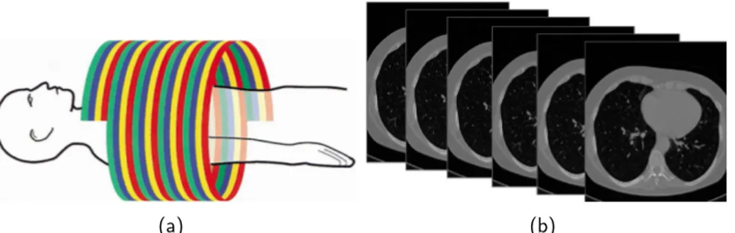
1.1.1 a) Example of bremsstrahlung and characteristic radiation spectra for different kV and mAs. b) Scheme of an X-ray vacuum sealed tube, with a rotating anode. . . 21 1.1.2 a) Path described by the X-ray tube in helical CT b) The slices
generated by a computed tomography exam. . . 22 1.1.3 Three orthogonal projections of a CT scan. . . 22 1.3.1 Figure representing the lung anatomy. . . 25 1.3.2 Slice of a chest CT exam. The principal organs and structures
are labeled: 1) Air outside the patient’s body, 2) Right lung, 3) Left lung, 4) Table of the scanner, 5) Trachea and large airways, 6) Esophagus, 7) Rib, 8) Sternum, 9) Blood vessels, 10) Fat tissue (patient’s body), 11) Spine, 12) Scapula. . . 26 2.3.1 Examples of Receiver Operating Characteristic (ROC) and
Free Receiver Operating Characteristic (FROC) curves. . . . 29 2.5.1 Pictures representing an internal nodule. . . 32 2.5.2 Pictures representing a juxta-pleural nodule. . . 33 2.5.3 Flowchart of the CAD sub-systems for internal nodule and
juxta-pleural nodule detection. . . 34 2.6.1 a) Screenshot of an image as seen in the OsiriX software. b)
A nodule annotated by the CAD system. The plugin window is visible in the right part of the image. . . 35 3.2.1 Diameter of the nodules annotated in the 20 ITALUNG − CT
CT scans. . . 38 3.3.1 Slice thickness of the CT scans of LIDC1 and LIDC2 datasets. 41
8 LIST OF FIGURES 3.3.2 LIDC1 and LIDC2 internal nodule size distributions. . . 42 3.3.3 LIDC1 and LIDC2 juxta-pleural nodule size distributions. . . . 43 3.4.1 Diameters of the nodules contained in the five example CTs of
the ANODE09 dataset. . . 44 4.3.1 Steps of the identification of the low intensity voxels inside the
patient’s body a) Thresholding between Sup and Slow: the low intensity voxels are labeled as foreground b) Connect compo-nent and labeling operation. The labels are shown in different gray levels c) Selection operation: the biggest connected com-ponent not lying on the boundary of the image is selected, whereas the others are discarded. . . 49 4.3.2 Rendering of the low intensity voxels obtained in first step of
the segmentation procedure. . . 50 4.4.1 Air segmentation: the connected component found selecting
those voxels with intensity ≤ TAir. a) In axial view connected components are shown in different gray levels b) the same connected components of a) viewed in coronal view. . . 52 4.4.2 Sketch representing the idea of the Hough transform for circles:
the black circle C is the one to be detected, while the three dotted circles of radius r and centers (x1, y1), (x2, y2), (x3, y3) are circles drawn in the parameter space. As shown in the figure, the point where the three red circles intersect is the center of C. . . 53 4.4.3 Rendering of the mask T, representing the trachea and the
large airways. . . 54 4.5.1 a) The anterior lung junction b) The anterior lung junction
where the maximum cost path, found in the lung separation step, is superimposed. . . 55 4.6.1 a) The segmented lung before vessels and airway walls removal
b) The segmented lung after vessels and airway walls removal 56 4.7.1 Rendering of the lung segmentation mask. . . 58 4.8.1 Flow Chart representing the lung segmentation process. . . 59
LIST OF FIGURES 9 5.3.1 Analytic and numeric response curve of the MSDE filter. The
filter settings are d0 = 4, d1 = 7 with N = 5 (number of multiscale steps). The filter is run on Gaussian blobs with diameter in the range [0, 10 mm]. From the picture is visible that the filter response is almost flat in the interval [5, 9 mm]. 64 5.4.1 Result of the SSDE filter run with a fixed scale d = 7 mm on
Gaussian blobs with diameters in the range [0, 40] mm. The zdot function from eq. (5.4.3) and the zdot obtained from tests on artificial objects are shown. . . 66 5.4.2 Result of SSDE filter applied to a blob of diameter 5 mm.
The filter is run with scale parameter varying in the range [0, 40] mm. The znorm function from eq. (5.3.1) and the znorm obtained from tests on artificial objects are shown. . . 67 6.2.1 The 15 unique combinations of the marching cube algorithm. . 72 6.4.1 Pictures representing the matrix S(x, y, z): each voxel
accumu-lates a score proportional to the number of normals passing through it. . . 74 6.5.1 Artificial objects used for testing the PSN filter. . . 75 6.5.2 PSN filter results on artificial objects of radius in the range[0, 20] mm,
the parameter of the filter l in this test is equal to the radius of the object. . . 75 6.5.3 Picture showing the normals computed on the pleura surface.
The blue circle underlines a juxta-pleural nodule. . . 76 7.2.1 Example of a candidate nodule segmentation: a) a nodule, b)
the corresponding segmentation. . . 78 7.3.1 Basic idea of the VBNA false positive reduction: each voxel is
characterized by a feature vector constituted by the intensity values of its 3D neighbors (5 × 5 × 5). . . 81 8.2.1 Results in terms of the Area Under the ROC curve (AUC) of
the SVM training on the LIDC1 with the features extracted by the CADI as a function of the penalty parameter C. . . 87 8.2.2 FROC curves obtained by the CADI at the four Agreement
10 LIST OF FIGURES 8.2.3 a) Rendering of the MSDE filter results applied to a CT scan.
The voxels with higher score are colored in red. b) One slice
of the CT scan shown in a). . . 88
8.2.4 Results in terms of AUC of the Support Vector Machine (SVM) training on the LIDC1 with the features extracted by the CADJP as a function of the penalty parameter C. . . 90
8.2.5 FROC curves obtained by the CADJP at the four ALs in LOPO mode on the LIDC1 (as described in sec. 3.3). . . 91
8.2.6 a) Rendering of the results of the Pleura Surface Normal (PSN) filter applied to a Computed Tomography (CT) scan. The vox-els with higher score are colored in red. b) One slice of the CT scan shown in a). . . 92
8.3.1 Results in terms of AUC of the SVM training on the LIDC2 with the features extracted by the CADI as a function of the penalty parameter C. . . 94
8.3.2 FROC curves obtained by the CADIon the LIDC2 at the four ALs in Leave One Patient Out (LOPO) mode. . . 95
8.3.3 Results in terms of AUC of the SVM training on the LIDC2 with the features extracted by the CADJP as a function of the penalty parameter C. . . 97
8.3.4 FROC curves obtained by the CADJP on the LIDC2 at the four ALs in LOPO mode. . . 98
8.6.1 Four example FP findings generated by the CADI. . . 103
8.6.2 Four FP findings generated by the CADJP. . . 104
B.3.1Pictures representing a neuron and MLP. . . 119
List of acronyms
AL Agreement Level
ANN Artificial Neural Network AUC Area Under the ROC curve CAD Computer Aided Detection CADI CAD for internal nodules CADJP CAD for juxta-pleural nodules CT Computed Tomography
DICOM Digital Imaging and Communications in Medicine format FLD Fisher Linear Discriminator
FP False Positive FN False Negative
FROCSV Free Receiver Operating Characteristic Score Value FROC Free Receiver Operating Characteristic
GGO Ground Glass Opacity HU Hounsfield Unit
IN Internal Nodule
JPN Juxta-Pleural Nodule
12 LIST OF FIGURES LDCT Low Dose Computed Tomography
LIDC Lung Image Database Consortium LOO Leave One Out
LOPO Leave One Patient Out MIP Maximum Intensity Projection MRI Magnetic Resonance Imaging MSDE Multi Scale Dot Enhancer NLST National Lung Screening Trial PET Positron Emission Tomography PSN Pleura Surface Normal
ROC Receiver Operating Characteristic ROI Region of Interest
SPECT Single Photon Emission Tomography SSDE Single Scale Dot Enhancer
SVM Support Vector Machine TN True Negative
TP True Positive
Introduction
Lung cancer is one of the main public health issues in developed countries. The overall 5-year survival rate is only 10−16% [1–4], although the mortality rate among men in the United States has started to decrease by about 1.5% per year since 1991 and a similar trend for the male population has been observed in most European countries.
By contrast, in the case of the female population, the survival rate is still decreasing, despite a decline in the mortality of young women has been ob-served over the last decade [5, 6].
Approximately 70% of lung cancers are diagnosed at too advanced stages for the treatments to be effective [7]. The five-year survival rate for early-stage lung cancers (stage I, see appendix A), which can reach 70% [8], is sensibly higher than for cancers diagnosed at more advanced stages.
Lung cancer most commonly manifests itself as non-calcified pulmonary nod-ules. The CT has been shown as the most sensitive imaging modality for the detection of small pulmonary nodules, particularly since the introduction of the multi-detector-row and helical CT technologies [9]. Screening programs based on Low Dose Computed Tomography (LDCT) may be regarded as a promising technique for detecting small, early-stage lung cancers [10,11]. The efficacy of screening programs based on CT in reducing the mortality rate for lung cancer has not been fully demonstrated yet, and different and opposing opinions are being pointed out on this topic by many experts [12, 13]. However, the recent results obtained by the National Lung Screening Trial (NLST), involving 53454 high risk patients, show a 20% reduction of mortal-ity when the screening program was carried out with the helical CT, rather than with a conventional chest X-ray [14].
LDCT settings are currently recommended by the screening trial protocols. However, it is not trivial in this case to identify small pulmonary nodules,
14 LIST OF FIGURES due to the noisier appearance of the images in low-dose CT with respect to the standard-dose CT. Moreover, thin slices are generally used in screening programs, thus originating datasets of about 300 − 400 slices per study. De-pending on the screening trial protocol they joined, radiologists can be asked to identify even very small lung nodules, which is a very difficult and time-consuming task. Lung nodules are rather spherical objects, characterized by very low CT values and/or low contrast. Nodules may have CT values in the same range of those of blood vessels, airway walls, pleura and may be strongly connected to them. It has been demonstrated, that a large percent-age of nodules (20 − 35%) is actually missed in screening diagnoses [15]. To support radiologists in the identification of early-stage pathological ob-jects, about one decade ago, researchers started to develop CAD methods to be applied to CT examinations [16–23].
Within this framework, two CAD sub-systems are proposed: CAD for inter-nal nodules (CADI), devoted to the identification of small nodules embedded in the lung parenchyma, i.e. Internal Nodules (INs) and CADJP, devoted the identification of nodules originating on the pleura surface, i.e. Juxta-Pleural Nodules (JPNs) respectively.
As the training and validation sets may drastically influence the performance of a CAD system, the presented approaches have been trained, developed and tested on different datasets of CT scans (Lung Image Database Consortium (LIDC), ITALUNG − CT) and finally blindly validated on the ANODE09 dataset.
The two CAD sub-systems are implemented in the ITK framework [24], an open source C++ framework for segmentation and registration of medical im-ages, and the rendering of the obtained results are achieved using VTK [25], a freely available software system for 3D computer graphics, image processing and visualization. The Support Vector Machines (SVMs) are implemented in SVMLight [26]. The two proposed approaches have been developed to detect solid nodules, since the number of Ground Glass Opacity (GGO) contained in the available datasets has been considered too low.
This thesis is structured as follows: in the first chapter the basic concepts about CT and lung anatomy are explained. The second chapter deals with CAD systems and their evaluation methods. In the third chapter the datasets used for this work are described. In chapter 4 the lung segmentation algo-rithm is explained in details, and in chapter 5 and 6 the algoalgo-rithms to detect internal and juxta-pleural candidates are discussed. In chapter 7 the
reduc-LIST OF FIGURES 15 tion of false positives findings is explained. In chapter 8 results of the train and validation sessions are shown. Finally in the last chapter the conclusions are drawn.
The original contributions in this work are the following:
• The efficient implementation of the algorithm described in 5.5.2. • The implementation of the CADJP, since it differs from [27, 28] in the
way the normals to the pleura surface are computed and the nodule candidates are classified.
• New features are added to the classification procedure with respect to the implementation described in [17, 19, 22], and a new classifiers SVM is used.
• The lung segmentation described in chap.4 may be regarded as par-tially original, since it puts together different pre-existing procedures described in [29–31].
Part I
Preliminaries
Chapter 1
Computed tomography
1.1
Computed Tomography
Computed tomography is a technique that allows to reconstruct a volume starting from a finite number of projections, each obtained using X-ray in-teraction with the target [32]. Modern Computed Tomography (CT) scanners typically employ a helical technology to scan the patient body, i.e. the table is translating while the X-ray source is rotating rapidly around the patient. The effect of this operation is that, in the frame of the table, the X-ray tube describes an helical path (see fig. 1.1.2).
Once reconstructed, a computed tomography chest exam is typically com-posed of 300 − 400 two dimensional images (according to the patient’s height and to the exam slice thickness). Each image is a slice of the reconstructed chest volume (see fig. 1.1.2).
The two dimensional images are gray level images containing, for each volume element, the reconstructed attenuation coefficient in Hounsfield Unit (HU). The value in HU of a material X, is defined as
HUX =
µX − µH2O µH2O
× 1000,
where µX is the X-ray linear attenuation coefficient of the tissue contained in the voxel and µH2O is the attenuation coefficient of water.
The attenuation coefficients depend on the energy of the X-ray passing through the material. Since the spectra of a X-ray tube (see fig. 1.1.1) is not monochromatic, the HU value of each tissue is weighted at each energy
20 CHAPTER 1. COMPUTED TOMOGRAPHY of the spectrum. Table (1.1) shows the HUs of some typical constituents of human body tissue.
The CT images are typically anisotropic, i.e. the voxels have different physi-cal dimensions vx, vy, vzwith vx= vy ∼ 0.6mm (referred as 2D pixel spacing) and vz> vx, vy (referred to as slice thickness) and vz varied, in the analyzed cases, between 0.6 and 5 mm.
The images are commonly stored in Digital Imaging and Communications in Medicine format (DICOM), a standard for handling, storing, printing, and transmitting information in medical imaging [33]. The DICOM files include a full dictionary of metadata (i.e. slice thickness, patient ’s orientation etc.) available together with the images.
Once the volume is reconstructed, it is possible to slice it in arbitrary planes. The most common planes for the visualization are those associated with the principal axes of the patient (see fig. 1.1.3).
In the X-ray tube (see fig. 1.1.1), a beam of electrons is first accelerated through a potential gap and then decelerated by hitting a solid piece of metal with a high atomic number. The electron beam is generated using a filament heated by Joule effect, which then emits electrons through ther-moionic emission.
The electrons are then accelerated across a potential gap, spanning between 40 kV to 150 kV, then strike the metallic target and produce X-ray radiation by bremsstrahlung and characteristic radiation.
The lower energy X-rays are absorbed within the X-ray tube, thus reducing the number of lower energy particles in the resultant spectrum. The theo-retical and “real like” spectra of an X-ray source for a thick target are shown in fig. 1.1.1.
The main advantages of CT over the ordinary radiography consists in the resolution obtained in the exam and in a fully 3D reconstruction of the volume of interest. However, a higher resolution has to be paid in terms of a higher radiation dose delivered to the patient.
There are plenty of parameters to roughly estimate the dose delivered by a CT exam, the most important are those related to the X-ray tube: the kV and the mAs. The kV is the value of potential gap that accelerates the electrons in the X-ray tube, corresponding also to the maximum energy of the photon emitted by bremsstrahlung, while the mAs are an abbreviation for milli-ampere per second and are the product between the filament current
1.2. EQUIVALENT AND EFFECTIVE DOSE 21
(a) (b)
Figure 1.1.1: a) Example of bremsstrahlung and characteristic radiation spectra for different kV and mAs. b) Scheme of an X-ray vacuum sealed tube, with a rotating anode.
Table 1.1: Hounsfield Units of some constituents of human body.
Substance HU Air -1000 Fat -120 Water 0 Muscle +40 Bone +400 or more
Pure lung tissue 50
Lung Parenchyma -600
and exposure time. There is no direct relation between dose and image noise, however the noise generally decreases while increasing the dose.
1.2
Equivalent and effective dose
Ionizing radiations cause an energy transfer to the target that is described by the quantity dose. In the international System of Units (SI) the dose is expressed in gray (Gy) where the gray is defined as the absorption of
22 CHAPTER 1. COMPUTED TOMOGRAPHY
(a) (b)
Figure 1.1.2: a) Path described by the X-ray tube in helical CT b) The slices generated by a computed tomography exam.
(a) Axial Slice (b) Coronal Slice (c) Sagittal Slice
1.3. LUNG ANATOMY AS SEEN IN A CT CHEST EXAM 23 Table 1.2: Table showing the value of wrfor alpha, beta and gamma radiations. Radiation type wr alpha 20 beta 1 gamma 1 protons (>2MeV) 5
one joule of ionizing radiations by one kilogram of matter. For a given dose radiations of different quality will induce different biological effects, e.g. one gray deposited by an alpha particle has a very different effect compared to one gray deposited by X-rays. For this reason a physical quantity called equivalent dose has been introduced:
H = wrD,
where D is the dose in gray and wr is a weighting factor that measures the particles delivering the dose. The unit of H is the sievert (Sv). Table 1.2 shows wr for alpha, beta and gamma radiations.
Since biological damage depends on the targeted organ, it is possible to define a physical quantity that accounts for different types of tissue
E = N !
t=0 wtHt
where wt are the weighting coefficients for different tissues and Ht the equiv-alent dose. E is referred to as effective dose and it is measured in sievert. Table 1.3 shows wt values for different tissues and effective doses delivered in different examinations.
1.3
Lung anatomy as seen in a CT chest exam
The lungs are a pair of spongy, air-filled organs located on either side of the chest and are wrapped in a thin tissue layer called pleura. As shown in
24 CHAPTER 1. COMPUTED TOMOGRAPHY Table 1.3: a) Weighting factor wt for different tissue [32] b) Effec-tive dose delivered by different examinations [14, 34].
(a) Tissue wt Lungs 0.12 Stomach 0.12 Skin 0.01 Gonads 0.2 (b)
Examination Effective dose (mSv)
Chest X-ray 0.1
Head CT 1.5
Chest CT 8
Low dose chest CT 1.5
Screening Mammography 3
fig. (1.3.1), the right lung is divided into three lobes whereas the left one is divided into two. The physical boundaries between lobes are called fissures. The trachea conducts inhaled air into the lungs through its tubular branches, called airways. The trachea is clearly visible in a CT chest exam as a tubular air-filled structure, near the head of the patient (see fig. 1.3.2).
Two branches of the airways, one for each lung, start from the trachea, and divide into smaller branches, finally becoming microscopic.
As reported in [35, 36], there are typically 23 generations of airways, and the relation between the trachea diameter d0 and the diameter dn of nth branch follows the scaling law:
dn = d02−
n
3. (1.3.1)
The eq. 1.3.1 holds up to the 16thgeneration, after this generation the diame-ter of the airways remains approximatively constant until the 23thgeneration. According to the data reported in [36], the diameter of the trachea for adult subjects is (18±2) mm, this number may slightly differ according to patient’s sex, age and height. Using eq. (1.3.1) for the first generation of airways, a diameter of (14 ± 1.6) mm is found.
In a CT scan, a lot of structures are clearly visible; the most important are the lungs, ribs, trachea, esophagus, heart, fissures, blood vessels and the airway walls. In the CT slice shown in fig. (1.3.2) some of the mentioned organs are labeled.
1.3. LUNG ANATOMY AS SEEN IN A CT CHEST EXAM 25
26 CHAPTER 1. COMPUTED TOMOGRAPHY
Figure 1.3.2: Slice of a chest CT exam. The principal organs and structures are labeled: 1) Air outside the patient’s body, 2) Right lung, 3) Left lung, 4) Table of the scanner, 5) Trachea and large airways, 6) Esophagus, 7) Rib, 8) Sternum, 9) Blood vessels, 10) Fat tissue (patient’s body), 11) Spine, 12) Scapula.
Chapter 2
Computer Aided Detection
systems
2.1
What is a Computer Aided Detection (CAD)
system?
CAD is a procedure that assists radiologists in the interpretation of medical images. Imaging techniques such as X-ray, MRI, and Ultrasound diagnostics yield plenty of information, which the radiologist has to analyze and evaluate comprehensively in a short time. CAD systems can help reading digital images, e.g. highlighting zones of the images which are suspected to contain a radiological sign of pathology (see fig. 2.6.1(b)).
CAD is a relatively young interdisciplinary technology combining elements of artificial intelligence and digital image processing with radiological image processing. A typical application is the detection of a tumor. Some hospitals use CAD to support radiologists in screening programs, e.g. as in mammog-raphy (for the diagnosis of breast cancer), and virtual colonoscopy (for the detection of polyps in the colon).
2.2
The role of CAD in a screening program
Screening is a strategy used in a high risk and asymptomatic population to detect a disease in individuals in absence of signs or symptoms of that disease.
28 CHAPTER 2. COMPUTER AIDED DETECTION SYSTEMS The purpose of a screening program is to identify a disease in early stage, thus enabling earlier intervention and management in the hope to reduce mortality and suffering from that disease. Although screening may lead to an earlier diagnosis, not all screening tests have been shown to benefit the population being screened; over-diagnosis, misdiagnosis, and creating a false sense of security are some possible negative effects of screening. For these reasons, a test used in a screening program, especially for a disease with low incidence, must have good specificity in addition to good sensitivity [37]. In a lung cancer screening context, it might be possible to use a CAD system in different modes to improve radiologists’s work, in particular the most common modalities are known as “first reader“ and “second reader”.
In first reader mode, the radiologists are allowed only to modify CAD find-ings. This mode is convenient when radiologists are asked to review a lot of images, most of those non pathological. Used in first reader mode the CAD is able to reduce reading time, and to prevent fatigue and inattentions. The main limitation of the first reader mode is that the radiologists’ upper bound on the sensitivity is given by the CAD performance. For this reason the use of a CAD as first reader is advised against in general, and limited to the use as an “image sorter”: the cases are selected by the CAD in order to be presented to radiologists, at first, those which are more probably pathological.
The most common use of a CAD system is the second reader mode. In the second reader mode, first radiologists read the exam “traditionally” and then with the help of the CAD. In principle this mode is slower than the first reader and the “traditional” modes, so this modality is acceptable only if it implies an enhancing of sensitivity at an acceptable rate of false positives.
2.3
How to evaluate a CAD performance
During the development and the validation of a CAD system, it is necessary to have a tool to compare its performance with those of other CADs or hu-man readers. For this purpose, it is common to use two different figures of merit: Receiver Operating Characteristic (ROC) and Free Receiver Operat-ing Characteristic (FROC) curves (see fig. 2.3.1), accordOperat-ing to the task to be evaluated [38].
In this section, the word “observer”, may refer both to CADs and to human readers, since the same considerations apply to both cases.
2.3. HOW TO EVALUATE A CAD PERFORMANCE 29
(a) ROC (b) FROC
Figure 2.3.1: Examples of ROC and FROC curves.
The ROC curve is used when binary classification is required, e.g. when an observer is asked to separate highly suspicious images for cancer from non pathological images. For such a kind of task, the observer is not asked to give only a binary answer, but to provide also a degree of suspicion p, e.g. a number in the [0, 1] range, representing the confidence of its choice.
Once a set of images is processed by the observer, it is possible to evaluate its performance, varying a threshold t between 0 and 1, and evaluating for each t the number of True Positive (TP), False Positive (FP), True Negative (TN) and False Negative (FN) findings, with p ≥ t (see tab. (2.1)).
The ROC curve is obtained, evaluating the sensitivity = TP/(TP + FN) and the specificity = TN/(TN + FP) for each t, and plotting the sensitivity vs (1 − specificity).
The Area Under the ROC curve (AUC) is a good estimate of the observer performances, since its value is equal to the probability that a randomly chosen positive example is ranked higher than a randomly chosen negative example [39].
However, the ROC curve is not an optimal tool to evaluate tasks where the spatial identification of lesions is not trivial. For example, identifying all the lung nodules in a CT scan is not trivial, since there are lots of structures that mimic nodules and real nodules may be very subtle to detect.
30 CHAPTER 2. COMPUTER AIDED DETECTION SYSTEMS Table 2.1: Table showing all the possible outcomes of a test.
Test result Gold standard
Positive Negative
Positive True Positive False Positive Negative False Negative True Negative
in the evaluation of the observer performances. This operation is typically carried out with the FROC analysis. In FROC the observer is asked to provide both a location and a degree of suspicion for each identified lesion. If an annotated mark is not close enough to “real lesions”, the mark is regarded as a FP. The main difference between the FROC and the ROC analysis, is that in the FROC the reader is free to annotate, in principle, an unlimited number of lesions. For this reason, it is not straightforward to compare two FROC curves as in the case of ROC curves. The FROC curve is obtained plotting the sensitivity versus the number of FP, similarly as for the ROC curve.
In this thesis, the FROC curves are compared using the criterion proposed in [17]: the values of sensitivity at seven predefined FP/CT rate (1/8, 1/4, 1/2, 1, 2, 4, 8) are averaged. The FROC analysis requires a localization criterion to be defined. In this thesis, a mark is considered corresponding to a nodule if its Euclidean distance from the annotated center is less than 1.5 times the radius of the annotated nodule.
2.4
The problem of the “gold standard”
In order to carry out FROC and ROC analysis, it is necessary to have a quality reference standard to compare with the method to be tested. In par-ticular, to assess the performance of CAD systems for lung nodule detection, the list of nodule locations annotated by radiologists is needed.
The creation of the reference standard is carried out using the so called “gold standard”, i.e. the most accurate exam that is able to detect a certain pathology.
2.5. CAD SYSTEM ARCHITECTURE 31 Opposite to other cases, e.g. breast cancer, the “gold standard” for detection of lung cancer cannot be based on histological exams, since lung biopsy is a dangerous procedure for the patient, and it is carried out only for big nodules and nodules strongly suspected to be cancer. Therefore, in principle, the biopsy would not be applicable to detect early cancers in asymptomatic population.
For this reason, the most accurate and less invasive exam for early lung cancer detection is a chest CT red by expert radiologists. However, since the inter-reader variability is very high for this kind of task, the problem of finding a “gold standard” for a certain number of cases is not as easy as it might seem in principle. this problem many solutions were proposed, but the discussion on this topic is nowadays still open.
The most common choice to create a reference standard is to form a panel of experts to review each scan, first independently and then, in case of dis-agreement, to jointly come together to arrive at a consensus decision. This solution is very difficult to apply in many cases and consensus panels are frequently believed to reflect the opinion of the “strongest” member of the panel [40]. Moreover, in forced consensus studies the inter-reader variability is completely lost.
To overcome these problems, the Lung Image Database Consortium (LIDC) [41] adopted a new reading modality. The LIDC designed a two-phase data collection process that allows multiple expert readers to review each CT scan, first independently (reading phase) and then, with their own and all the blinded annotations of the other readers (unblinded reading phase). Using this method, readers are free to adjust their own annotations without being forced to change them. At the end of this procedure there is no forced consensus, and the final reports contain, separately, for each case, all the unblinded marks of all the readers.
2.5
CAD system architecture
It is convenient, for detection purpose, to divide lung nodules in two differ-ent categories, according to their location and morphology: internal nodules and juxta-pleural nodules. Internal nodules (see fig. 2.5.1) originate in the lung parenchyma and can be regarded as spherical objects fully embedded into it, whereas juxta-pleural nodules (see fig. 2.5.2) originate on the pleural
32 CHAPTER 2. COMPUTER AIDED DETECTION SYSTEMS
(a) Rendering of the internal part of lung, in red is shown an internal nodule
(b) A CT image containing an in-ternal nodule
Figure 2.5.1: Pictures representing an internal nodule.
surface and can be modeled as hemispherical objects. Since these two main categories are very different, the proposed approach implements two different procedures, each devoted to the identification of one typology of nodules:
• CADI for the identification of internal nodules;
• CADJP for the identification of juxta-pleural nodules.
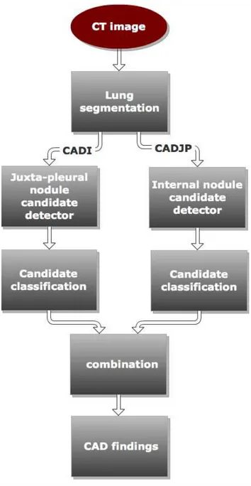
The two CADs share the lung segmentation procedure described in chap.4. After the lung segmentation two procedures devoted to the identification of internal and juxta-pleural nodule candidates are implemented. The proce-dure to detect internal nodules candidates is described in chap.5, and it is based on a Hessian eigenvalues algorithm. The procedure to detect juxta-pleural candidates is described in chap.6 and it is based on the detection of candidates trough pleura surface normals. After the candidate detection, the classification procedures described in chap.7 are implemented. Finally the two CADs system are combined using the procedure described in 8.4. In fig. 2.5.3 a flowchart of the two CAD system procedures is shown.
2.6. OSIRIX PLUGIN 33
(a) Rendering of the pleura surface, in green is shown a juxta-pleural nodule
(b) A CT image containing a juxta-pleural nodule
Figure 2.5.2: Pictures representing a juxta-pleural nodule.
2.6
OsiriX plugin
In order to allow the annotation of the images and the visualization of the CAD findings, a dedicated plugin for the OsiriX DICOM viewer [42] has been implemented within the Cocoa environment of MacOSX. OsiriX is an open source DICOM image processing and visualization software for different imaging types, e.g. Magnetic Resonance Imaging (MRI), CT, Positron Emis-sion Tomography (PET), PET-CT, Single Photon EmisEmis-sion Tomography (SPECT)-CT, Ultrasounds, etc., which allows a simple mechanism for writ-ing plugins that expand its functionalities. The plugin allows annotatwrit-ing nodules and visualizing in different colors the separate CAD sub-system re-sults, their combination and the radiologists’ annotations. A screenshot of the plugin is shown in fig. 2.6.1.
Using the plugin, radiologists can visualize and process the CT data using all the tools included in the OsiriX software (zooming, changing the intensity windowing, browsing slices, Maximum Intensity Projection (MIP) projec-tions, etc.), identify nodules and annotate them. The annotations consist of simple circular Region of Interests (ROIs), identified by their center and ra-dius. Using the sliders it is also possible to select a working point, to visualize only findings above the selected thresholds.
34 CHAPTER 2. COMPUTER AIDED DETECTION SYSTEMS
Figure 2.5.3: Flowchart of the CAD sub-systems for internal nodule and juxta-pleural nodule detection.
2.6. OSIRIX PLUGIN 35
(a) (b)
Figure 2.6.1: a) Screenshot of an image as seen in the OsiriX software. b) A nodule annotated by the CAD system. The plugin window is visible in the right part of the image.
Chapter 3
Datasets
3.1
Introduction
As discussed in sec.2.4, to obtain a reliable annotated dataset of CT may re-quire a lot of effort. Therefore, it is natural to consider the data acquisition and annotation procedure a very important part of a CAD system develop-ment. Data coming from clinical environment are often not suitable to train or validate a CAD, since annotations provide qualitative explanation of the lesion position and type. For this reason, and many others, the typical choice to develop a CAD system is to rely on public datasets.
Results obtained on public datasets have the advantage to be directly com-parable with those present in literature, therefore, for scientific works, public datasets should be preferred. In this thesis three datasets, two of which are public, are used to train and to validate the proposed CAD scheme: the ITALUNG − CT, the LIDC and the ANODE09 database.
3.2
The ITALUNG − CT database
The presented CAD system has been originally developed and trained on a subset of the ITALUNG − CT database, collected by the Pisa center of the ITALUNG−CT trial, which is the first Italian randomized controlled trial for the screening of lung cancer [43]. The CT scans were acquired with a 4-slice spiral CT scanner (Siemens Volume Zoom) according to a low-dose protocol (tube voltage: 140 kV, tube current: 20 mA, mean equivalent dose 0.6 mSv),
38 CHAPTER 3. DATASETS
(a) Histogram of diameters of the inter-nal nodules.
(b) Histogram of the diameters of the juxta-pleural nodules.
Figure 3.2.1: Diameter of the nodules annotated in the 20 ITALUNG − CT CT scans.
with 1.25 mm slice collimation. Each scan is stored in DICOM format. Slices were reconstructed at 1 mm thickness, using a medium sharp reconstruction kernel (Siemens B50f). The number of slices per scan is approximately 300, each slice being a 512 by 512 pixel matrix, with pixel sizes ranging from 0.53 to 0.74 mm and 12 bit gray levels in Hounsfield Units. The annotations were marked by experienced radiologists participating to the Italian MAGIC-5 research project [44]. In this thesis, a dataset of 20 CT scans, containing 23 internal nodules and 15 juxta-pleural nodules with the size distribution shown in fig. 3.2.1, is used.
3.3
LIDC database
The LIDC database is the largest collection of annotated and publicly avail-able CTs. LIDC is a multi center and multi manufacturer database, with cases of different collimation, kV and tube current and reconstructed with different slice thickness.
On the contrary to the previous release of the LIDC database, where the annotations were obtained by a forced consensus among different readers, in the current release, to capture the inter-reader variability, four different
3.3. LIDC DATABASE 39 annotations made by four expert radiologists for each case in a two phase reading modality are provided, as explained in sec.2.4.
The LIDC annotations contain three kinds of objects [45]: nodules with di-ameters ≥ 3 mm, nodules with didi-ameters < 3 mm and “non nodules” with diameters > 3 mm. The contours of the objects marked as nodules with diameters ≥ 3 mm are provided for every reader together with eight subjec-tive characteristics in a 1 − 5 scale: subtlety, internal structure, calcification, sphericity, margin, spiculation, texture, malignancy. For nodules with diam-eters < 3 mm and non nodules with diamdiam-eters > 3 mm only a centroid is provided and no information on the size is available.
However, for a detection purpose LIDC data are redundant, since only a centroid and an estimate of the lesion size are needed.
Starting from the annotated contours, it is possible to obtain the information needed with many different algorithms. However, in order for the results to be directly comparable with those of literature, the annotations provided by the Cornell University [46] are used. These annotations are built with the purpose to be a reference standard to compare results of different data groups, and are generated according to the prescriptions given in [47]. First, the correspondence among contours drawn by different readers are eval-uated: a mask containing all the lesion voxels is generated starting from each contour, then the masks with at least one voxel in common are considered referring to the same object.
To evaluate the center and the dimension of a lesion, first each contour re-ferring to a lesion is assigned a center of mass, then the median value of the center in each direction provides the center of the lesion.
To estimate the size of the lesion, the volume of voxels contained in each contour is evaluated, and the median volume is considered the volume of the lesion. To obtain an estimation of the nodule size, the diameter of the sphere having the same volume as the nodule estimated volume is evaluated, i.e.
diameter = 2 ·" 3 · V 4π
#13
where V is the estimated volume of the lesion.
It is common to report the results on this database using four Agreement Level (AL) among the single reader annotations, i.e. considering the nodules
40 CHAPTER 3. DATASETS Table 3.1: Number of nodules in the datasets LIDC1 and LIDC2 divided by category.
Dataset Internal Nodule (IN) (relevant/irrelevant) Juxta-Pleural Nodule (JPN) (relevant/irrelevant)
LIDC1 137 (96/41) 72 (42/30)
LIDC2 137 (95/42) 36 (19/17)
Table 3.2: Number of nodules in the datasets LIDC1 and LIDC2 divided by AL.
Dataset AL 1 AL2 AL3 AL4 number of CTs
LIDC1 209 138 98 67 69
LIDC2 173 114 86 42 69
annotated by at least one (AL1), two (AL2), three (AL3) and four radiologists (AL4).
At present, the LIDC database contains 1000 CTs. However, in this thesis, only 138 CT scans are used. The 138 CTs result from selecting cases with slice thickness ! 2 mm, without contrast media and annotation included in the Cornell University report. The 138 CTs were divided in two subsets named LIDC1 and LIDC2, consisting of 69 CTs each.
Nodules with AL1 are referred to as irrelevant in this thesis, since all the training procedure is carried out using nodules with at least AL2.
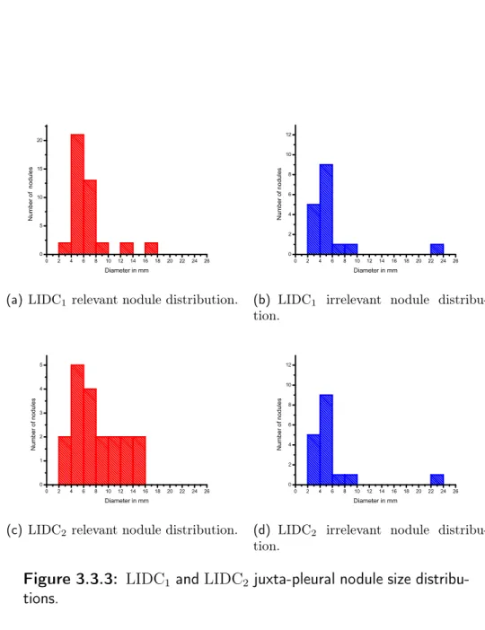
Table 3.1 shows the number of nodules contained in the two subsets, divided into two categories. Table 3.2 shows the agreement level for the datasets LIDC1 and LIDC2. In fig. 3.3.1 the slice thickness of the two subsets are shown.
Figures 3.3.2 and 3.3.3 show the nodule diameter distributions for relevant and irrelevant nodules. Since the LIDC annotations provide no information on the nodule typology, the nodules are divided in two categories, namely internal or juxta-pleural, on the basis of visual assessment.
3.4. ANODE09 DATABASE 41
(a) Slice thickness distribution of the LIDC1
dataset.
(b) Slice thickness distribution of the LIDC2
dataset.
Figure 3.3.1: Slice thickness of the CT scans of LIDC1 and LIDC2 datasets.
3.4
ANODE09 database
The ANODE09 [48] is an international initiative devoted to compare objec-tively different CAD systems, able to perform automatic detection of pul-monary nodules in chest CT scans on a single common database, with a single evaluation protocol. Data is provided by the Nelson study, the largest CT lung cancer screening trial in Europe. The images, acquired according to a low dose protocol, have slice thickness between 0.7 and 1 mm and an average number of slices equal to 430. Any team, whether from academia or industry, can join this study. The database of this study consists in five example CTs with publicly available annotations and 50 low dose thin-slice CT scans without public availability of the annotations. The 50 CTs are intended as a validation dataset, so it is forbidden to use these data to train any CAD system. The only information known about the 50 CTs, is the distribution of the nodule diameters: 40% of the nodules are below 4 mm in diameter, 40% have a diameter between 4 and 6 mm and 20% are larger. Since annotations for the 50 CT scans are not publicly available, all the findings must be inserted in a file together with their coordinates and degree of suspicion, and uploaded to the ANODE09 website [48], to receive in return the FROC curves.
42 CHAPTER 3. DATASETS
(a) LIDC1 relevant nodule distribution. (b) LIDC1 irrelevant nodule distribu-tion.
(c) LIDC2 relevant nodule distribution. (d) LIDC2 irrelevant nodule
distribu-tion.
3.4. ANODE09 DATABASE 43
(a) LIDC1 relevant nodule distribution. (b) LIDC1 irrelevant nodule distribu-tion.
(c) LIDC2 relevant nodule distribution. (d) LIDC2 irrelevant nodule
distribu-tion.
Figure 3.3.3: LIDC1 and LIDC2 juxta-pleural nodule size distribu-tions.
44 CHAPTER 3. DATASETS
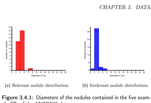
(a) Relevant nodule distribution. (b) Irrelevant nodule distribution.
Figure 3.4.1: Diameters of the nodules contained in the five exam-ple CTs of the ANODE09 dataset.
allows for a direct comparison.
As discussed in sec. 2.3, to extract a single score value from the FROC curve, the average sensitivity at seven predefined false positive rates is computed: 1/8, 1/4, 1/2, 1, 2, 4, and 8 FP/CT. This value is referred to as Free Receiver Operating Characteristic Score Value (FROCSV) in the following sections. The nodules of the ANODE09 dataset are divided into six categories ac-cording to their location and shape, thus allowing a more accurate scoring of each category independently: nodules bigger than 5 mm, nodules smaller than 5 mm, isolated nodules, juxta-pleural nodules, juxta-vascular nodules and peri-fissural nodules.
The dataset contains also irrelevant findings, i.e. findings that are counted neither as FP nor as TP in the evaluation of the FROC curve. There are three types of irrelevant findings: findings that mimic a nodule but that an expert observer believes not to be a nodule, nodules with benign characteristics and nodules that are too small to be relevant.
The nodules contained in the five example CTs were divided, according to visual assessment, into internal nodules and juxta-pleural nodules, thus re-sulting in 36 relevant internal nodules and only three relevant juxta-pleural nodules.
Part II
Image analysis algorithms
Chapter 4
Lung segmentation
4.1
Introduction
In computer vision, segmentation refers to the process of partitioning a digi-tal image into multiple segments, i.e. sets of pixels. The goal of segmentation is to simplify and/or change the representation of an image into more mean-ingful and easier information to analyze. In this case, the lung segmentation module of the CAD is essential to avoid marking findings outside lungs, and to provide an accurate representation of the pleura surface, necessary to detect juxta-pleural nodules. Since segmentation methods always rely on anatomical models, the information provided in sec. 1.3 is often used in this chapter.
The chapter is organized as follows: first, the image preprocessing and the algorithm to find low intensity voxels inside the patient body are shown, then the algorithm for the trachea and large airways segmentation and then the algorithm to separate the lungs and to fill vessels and airways are described, finally, the results obtained on a subset of the LIDC dataset are shown.
4.2
Image preprocessing
Shape identifier and morphological algorithms are designed to work better with isotropic images, i.e. images with cubic voxels. However, as it is dis-cussed in sec. 1.1, CT images are typically anisotropic. To improve the
48 CHAPTER 4. LUNG SEGMENTATION performances of morphological and shape identifier filters, an isotropization procedure is implemented.
Among many possible and arbitrary choices to resample the CT volume, it was chosen to resample the image in order to obtain a spacing of 1 mm and to smooth the image with a Gaussian kernel proportional to the original spacing of the images, as suggested in [24, 49].
4.3
Identification of low intensity voxels inside
the patient’s body
To identify the low intensity voxels inside the patient body, a procedure similar to [29] is implemented. This procedure consists in a simple thresh-olding [50] between Sup = −600 HU and Slow = −1000 HU followed by a tridimensional connected component labeling. Then, searching the biggest connected component not lying on the boundary of the volume (see fig. 4.3.1) provides the lungs together with air voxels contained in the trachea and the large airways. If two connected components, with a volume ratio of at least 0.5 are found, the algorithm goes to the “vessel and airway walls removal” and the lungs are considered to be separated.
The output of this procedure is a mask M where the low intensity voxels are labeled as foreground, i.e. are set to 1, while the rest of the image is labeled as background, i.e. is set to 0.
As shown in fig. 4.3.2, the air voxels inside the trachea act as a bridge between the two lungs. To obtain the segmentation for each lung separately, it is necessary to segment out from M the trachea and the large airways.
4.4
Trachea segmentation
Trachea segmentation is a relatively common task in lung CT segmentation. There are plenty of algorithms available in literature to segment trachea, the presented approach is a mixture of different elements, with the purpose of roughly identifying the trachea and the large airways connected to it.
4.4. TRACHEA SEGMENTATION 49
(a) (b) (c)
Figure 4.3.1: Steps of the identification of the low intensity voxels inside the patient’s body a) Thresholding between Sup and Slow: the low intensity voxels are labeled as foreground b) Connect component and labeling operation. The labels are shown in different gray levels c) Selection operation: the biggest connected component not lying on the boundary of the image is selected, whereas the others are discarded.
The algorithm is divided into four steps: • optimal threshold identification;
• threshold and connect component analysis;
• search of connected component representing the trachea; • trachea removal.
Optimal threshold identification
To segment out from M the trachea and the large airways, a two materials decomposition approach is implemented [30]. This approach relies on the hypothesis that the voxels contained in the mask M can be divided into two categories: lung voxels and air voxels. Since trachea and large airways are mostly filled with air, the first step to identify them is to find all the voxels of air contained in M.
In particular, assuming that the lungs are composed by air and lung tissue, it is possible to write the two material decomposition formula
50 CHAPTER 4. LUNG SEGMENTATION
Figure 4.3.2: Rendering of the low intensity voxels obtained in first step of the segmentation procedure.
4.4. TRACHEA SEGMENTATION 51 nMH¯M = nAirH¯Air+ nLungH¯Lung (4.4.1) where ¯HM, ¯HAir, ¯HLung are respectively the average density of the voxels on the mask M, the average intensity of the air and the average intensity of the lung tissue, and nAir, nLung, nM are respectively the number of air voxels, the number lung tissue voxels and the total number of voxels in M, with
nM = nAir+ nLung. (4.4.2)
Given ¯HAir, ¯HLung, and using eq. 4.4.2, it is possible to obtain nAir inverting eq. 4.4.1 nAir = nM ¯ HM − ¯HLung ¯ HAir− ¯HLung .
By evaluating the histogram of HU values included in the mask M, it is possible to find the threshold TAir so that
TAir = max T ∈[Tmin,Tmax]{n
T ≤ nAir}
where nT is the number of voxels, inside the mask M with intensity values ≤ T and Tmin and Tmax are the maximum and minimum values of the voxels inside M. The values of ¯HAir = −999 HU and ¯HLung = +48 HU are selected according to the prescription given in [30].
Threshold and connected component analysis
Once TAir is found, to identify all the air voxels inside the mask M, a thresh-olding operation between Tmin and TAir is applied. Then a connect compo-nent analysis is able to discard all the isolated air voxels. The results of this operation is shown in fig. 4.4.1, where a connected component representing the trachea is clearly visible.
Search of connected component representing the trachea
To identify the trachea among all the connected components shown in fig. 4.4.1, a circular 2D shape, corresponding to the trachea axial section, is searched near the head of the patient, i.e. in the upper central region of the CT. The identification of the circular section is carried out using the Hough transform for circle [50].
52 CHAPTER 4. LUNG SEGMENTATION
(a) Axial view (b) Coronal view
Figure 4.4.1: Air segmentation: the connected component found selecting those voxels with intensity ≤ TAir. a) In axial view con-nected components are shown in different gray levels b) the same connected components of a) viewed in coronal view.
The Hough transform is an operation that allows the identification of different shape classes (e.g. line, circles, ellipses, etc etc...) in binary images, using a voting procedure. The voting procedure is carried out in a parameter space, and the object candidates are obtained as local maxima in a so-called accumulator space, constructed by the algorithm for computing the Hough transform. A simple explanation of the Hough transform follows.
Hough transform for circles of known radius
Suppose that a circle C of known radius r has to be found in a bidimensional image.
The parametric form of the C is written x = r · cos(θ) + a
y = r · sin(θ) + b (4.4.3)
where θ ∈ [0, 2π] is a polar angle and a,b are the coordinates of the circle center.
Inverting the eq. 4.4.3 with respect to a and b, yields to a = x − r · cos(θ)
b = y − r · sin(θ) (4.4.4)
4.4. TRACHEA SEGMENTATION 53 x1, y1 x2, y2 x3, y3 r r r r
Figure 4.4.2: Sketch representing the idea of the Hough transform for circles: the black circle C is the one to be detected, while the three dotted circles of radius r and centers (x1, y1), (x2, y2), (x3, y3) are circles drawn in the parameter space. As shown in the figure, the point where the three red circles intersect is the center of C.
Since the radius of the circle to be found is known, the parameter space is two dimensional, i.e. the two dimensions are the coordinated (a, b). According to the transform eq. 4.4.4, each point (x, y), lying on C, becomes a circle of radius r itself in the parameter space.
Each pixel in the parameter space accumulates a score proportional to the number of circles passing through it (see fig. 4.4.2). Once this procedure is applied, the center of C is given by the pixel that accumulates the higher score.
Hough transform for circles of unknown radius
If the radius of the circle to be found is not known, the procedure is similar, except that the range [rmin, rmax] of allowed radii is spanned. Then for each r ∈ [rmin, rmax], the Hough procedure with a known radius is repeated. To apply the Hough algorithm to the trachea identification, first a morpho-logical operation to evaluate the border of the mask is implemented, and then the Hough transform is applied on the upper central region of the CT image. The pixel with highest score in the accumulator is then used as the seed to identify the trachea, while the other connected components are discarded.
54 CHAPTER 4. LUNG SEGMENTATION
Figure 4.4.3: Rendering of the mask T, representing the trachea and the large airways.
Following the prescriptions given in sec. 1.3, values of rmin = 7 mm and rmax = 11 mm for the trachea radius are selected, and it is chosen, on the basis of experiments, to search the trachea only in the upper 10% of the slices and in a band of 20 mm around the image center. The output of this procedure is the mask T shown in fig. 4.4.3.
Trachea removal
Once the trachea and the large airways are correctly identified, a dilation operation with a spherical kernel of radius 2 mm is applied to the mask T to include the high intensity walls of trachea and the airways. Then each voxel belonging to the dilated T mask is deleted from the mask M, thus generating a new mask M1.
At the end of this procedure lungs may be still fused, due to the low inten-sity of the anterior and posterior junction. In case of failure, a dedicated procedure is implemented to identify lung junctions.
4.5. LUNG SEPARATION 55
(a) (b)
Figure 4.5.1: a) The anterior lung junction b) The anterior lung junction where the maximum cost path, found in the lung separation step, is superimposed.
4.5
Lung separation
If the lungs are still fused, a dedicated procedure similar to that reported in [31,51] is implemented. The procedure search, for each slice, the maximum path weighted on HU between the anterior and posterior part of the patient. This method relies on the assumption that the junction tissue has a larger HU value compared to the tissue generally contained in the mask M1. The junction lines are searched only in band of size s = 30 mm near the center of mass of the segmented region contained in M1. Before starting the path search, the voxel values outside the mask M1 are set to +2000, in order to prevent the path to enter in the lungs when it’s not necessary.
The maximum cost of the path is evaluated using a dynamic programming approach [52]. The results of this procedure are shown in fig. 4.5.1. Once the optimal path is found, the voxels belonging to it are subtracted from the M1 mask and the connected components are searched with a 6-pixel connectivity rule.
56 CHAPTER 4. LUNG SEGMENTATION
(a) (b)
Figure 4.6.1: a) The segmented lung before vessels and airway walls removal b) The segmented lung after vessels and airway walls removal
4.6
Vessels and airway walls removal
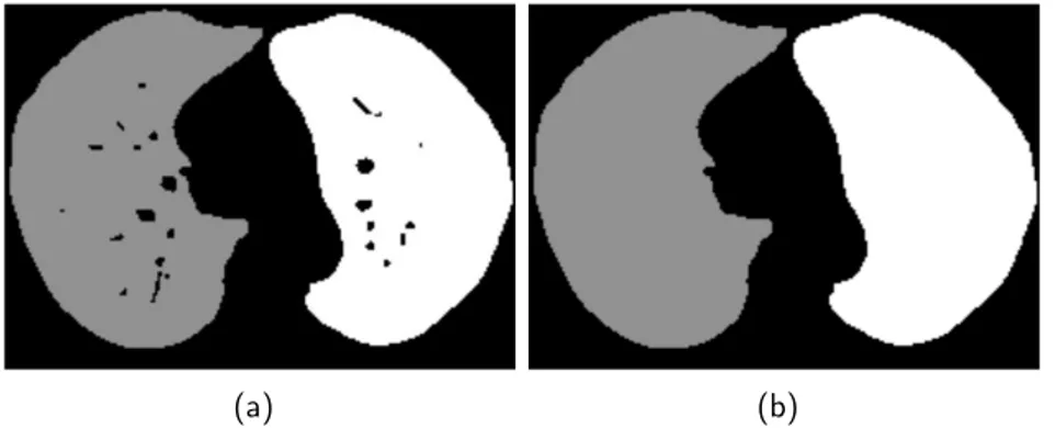
As shown in fig. 4.6.1, vessels and airways walls are not included in the seg-mented lung at this stage. To include them without modifying the pleura surface morphology, i.e. without modifying the shape of the juxta-pleural nodules, a combination of morphological operators is applied [50]. In par-ticular, a sequence of the dilation and the erosion operators with spherical kernels rdand re, with re > rdis applied. Finally, the logical OR operation be-tween the obtained mask and the original lung mask provides the final mask, where the vessels and the airway walls are filled in, while maintaining the original shape of the lung mask border [22]. The shape of the juxta-pleural nodules is not modified by this procedure (see fig. 4.6.1). Once removed vessels and airways, the pleura surface is defined as the surface separating parenchyma from the rest of the image (see fig. 4.7.1).
The optimal parameter rd= 8 mm is chosen to fill holes whose dimension is approximatively equal to that of the first generation of airways (see sec.1.3). Whereas the parameter rd = 16 mm is chosen to erode the pleura surface of 16 mm more than the dilation operation, thus avoiding to undersegment juxta-pleural nodules with a radius up to 16 mm.
4.7. AUTOMATIC ERROR CHECK 57
4.7
Automatic error check
The segmentation of anatomical structures in CT scans is a challenging task in medical imaging. Therefore, it is reasonable to expect any algorithm to fail in some cases, due to small anatomical differences among patients and different parameters in image acquisition and reconstruction.
For this reason, it is important to implement a tool able to automatically check the organ segmentations and to assess, on the basis of observables, if the segmentations are likely to be correct or not.
The procedures to be checked against failures are the trachea segmentation and the lung separation.
The trachea segmentation is considered successful, when a connected com-ponent with a volume in the range of Vmin = 10000 mm3 to the Vmax = 70000 mm3 is found, otherwise the segmented region is discarded. The values Vmin and Vmax are chosen on the basis of the range of values found on the LIDC1 set described in sec. 3.3.
The trachea segmentation failure is mainly due to the selection of a threshold TAir unable to separate the trachea air from the lungs. The lung separation is checked against failure and the identified connected component are filtered according to their dimensions. The lungs are finally considered to be sepa-rated when two connected components with at least a volume ratio of 0.5 are found.
Failures in separation are mainly due to the fact that, separating lungs slice by slice, doesn’t imply a tridimensional separation. In case of failures, the de-fault behavior of the procedure consists in applying the fill vessels procedure explained in sec. 4.6 to the whole block including the two lungs.
4.8
Results
The segmentation algorithm is tested and optimized on a subset of LIDC consisting in 138 CTs from different centers and acquired with scanners from different manufacturers. The LIDC1 is used to set segmentation parameters, while LIDC2 is used to validate the results. In tab. 4.1, the results of the segmentation procedure are shown, the failure of the algorithm is assessed on the basis of the automatic error check and visual assessment.
58 CHAPTER 4. LUNG SEGMENTATION
Figure 4.7.1: Rendering of the lung segmentation mask. Table 4.1: Table showing the results of the segmentation procedure obtained on the LIDC subsets.
Procedure Dataset
LIDC1 LIDC2 Trachea segmentation failure 1/69 1/69
Lung separation failure 6/69 7/69
The results of this procedure show that the trachea segmentation fails once on the LIDC1 dataset, once on the LIDC2; whereas the lung separation pro-cedure fails on 6 cases of the LIDC1 and 7 of the LIDC2. In all the other cases, a good segmentation was achieved. The workflow of the segmentation algorithm is resumed in fig. 4.8.1.
These tests show that the segmentation is stable even though it can fail in some cases.
4.8. RESULTS 59
Figure 4.8.1: Flow Chart representing the lung segmentation pro-cess.
Chapter 5
Detection of internal nodules
5.1
Introduction
Hessian algorithms are very common image analysis, since they provide a robust tool to find shapes like cylinders or dots in bidimensional and tridi-mensional images. In this chapter the algorithm used to identify solid inter-nal nodules is shown. The chapter is organized as follows: first the Single Scale Dot Enhancer (SSDE) and Multi Scale Dot Enhancer (MSDE) algo-rithms [20] are explained, then an efficient implementation of the algorithm is described and the numerical results of the implemented MSDE together with the theoretical algorithm are shown.
5.2
Single Scale Dot Enhancer (SSDE) filter
As discussed in [20], Gaussian blobs are an effective model to represent in-ternal nodules. To enhance such a kind of objects inside the lung volume, a SSDE filter is implemented.
For example, in a tridimensional space the expression of a Gaussian is I(x, y, z) = H0 · exp(− x2 2σ2 x − y2 2σ2 y − z2 2σ2 z ). (5.2.1)
where H0 is a constant, σ2x, σy2, σz2 are the variances along the three axis of the Gaussian, i.e. the dimensions of the object.
62 CHAPTER 5. DETECTION OF INTERNAL NODULES According to the values assumed by σx, σy, σz, the function I(x, y, z) repre-sents different structures.
It is possible to distinguish three main cases:
1. Blob shape: The variances have the same order of magnitude, e.g. σx≈ σy ≈ σz ≈ σ, Iblob(x, y, z) = H0· exp(−x
2+y2+z2
2σ2 ).
2. Cylinder shape: One of the variances much bigger than the others, e.g. σx → ∞ represents a tubular structure with the axis parallel to the x axis Icylinder(x, y, z) ≈ H0 · exp(−y
2 2σ2 y − z2 2σ2 z).
3. Plane shape: two variances have σx → ∞ and σy → ∞, Iplane ≈ H0· exp(−z
2
2σ2 z).
By evaluating the Hessian matrix of eq. 5.2.1, the eq. 5.2.2 is obtained H(x, y, z) = (xσ24 x − 1 σ2 x) xy σ2 xσy2 xz σ2 xσ2z xy σ2 xσy2 ( y2 σ4 y − 1 σ2 y) yz σ2 yσ2z xz σ2 xσz2 yz σ2 yσz2 ( z2 σ4 z − 1 σ2 z) I(x, y, z) (5.2.2)
where H(x, y, z) is the matrix form of the eq. 5.2.3
Hi,j(x, y, z) = ∂i∂jI(x, y, z) (5.2.3) for i, j = 1, .., 3.
By computing H(0, 0, 0), i.e. evaluating H(x, y, z) in the Gaussian center, a diagonal matrix is obtained
H(0, 0, 0) = H0 −σ12 x 0 0 0 −σ12 y 0 0 0 −1 σ2 z . (5.2.4)
This means that the eigenvalues of the Hessian matrix, in the center of the Gaussian, are function of the sizes of the object to be enhanced. Thus, using the Hessian eigenvalues, it is possible to evaluate a score proportional to the probability to have a Gaussian shape centered in that point.
In practice, since the analytic form of H(x, y, z) is not known, the Hessian needs to be evaluated numerically, for example using a finite difference ap-proach or a recursive apap-proach [53]. Computing Hessian involves comput-ing derivatives. However, since derivatives without any prior smoothcomput-ing are known to enhance noise [54], it’s necessary to define a scale of interest.
5.3. Multi Scale Dot Enhancer (MSDE) FILTER 63 The definition of a scale of interest in computer vision is a fundamental concept, in order to give the algorithms an idea of the dimension of the objects to be searched. Once the eigenvalues λ1, λ2, λ3 of the Hessian matrix are evaluated for each voxel, it is possible to calculate the score
zdot(λ1, λ2, λ3) = *|λ 3|2 |λ1| if λ1, λ2, λ3 < 0 0 otherwise ; (5.2.5) where | λ1 |≥| λ2 |≥| λ3 |.
Evaluating the zdotvalue, for a blob, a cylinder and plane shapes, it is possible to show that the zdot vanishes in the center of the planar and cylindrical structures, while for blobs of variance σ2, z
dot(Iblob) ∼ σ12. This means that the SSDE is able to discriminate blobs from planar and cylindrical structures and that its score is inversely proportional to the magnitude of the blob. However since, in general, it is preferable to assign a comparable score to all the nodules in a certain range (e.g. from 3 mm to 10 mm in diameter), a multiscale approach has to be followed.
5.3
Multi Scale Dot Enhancer (MSDE) filter
The MSDE algorithm consists in combining, according to the prescription given in [20], the zdot functions evaluated at several scales. This procedure is based on an a priori knowledge of the sizes of the objects to be enhanced. For what concerns nodules, assuming that a nodule can be approximated by a 3D Gaussian with scale parameter σ, the nodule diameter can be denoted with 4σ, thus taking into account for more than 95% of the nodule volume. If the nodule diameters to be enhanced are in the range [dmin, dmax], the scales to be considered for the Gaussian filter are in the range [σmin, σmax], where σ = d/4. Within that range, the N intermediate scales are computed as σi = ri−1σmin where i = 1, .., N and r = (ddmaxmin)1/(N−1).
The resulting filter value is then:
znorm(σi) = σ2izdot(σi) (5.3.1)
zmax = max(znorm(σi)) (5.3.2)
with i = 1, .., N. The final output of the MSDE is a matrix, referred in the following section as Z(x, y, z), where each voxel contains the value of the obtained zmax. The range of diameters for the objects to be enhanced, and