The Pisa pre-main sequence stellar evolutionary models: results for non-accreting and accreting models

Graduate Course in Physics

University of Pisa

The School of Graduate Studies in Basic Science ”GALILEO GALILEI”

PhD Thesis:

The Pisa pre-main sequence

stellar evolutionary models:

results for non-accreting and

accreting models

Candidate

Supervisors

Emanuele Tognelli

Prof. Scilla Degl’Innocenti

Dr. Pier Giorgio Prada Moroni

Introduction v

Publications ix

1 Updating pre main sequence models 1

1.1 Overview . . . 1 1.2 Macro-physics . . . 4 1.2.1 Boundary conditions . . . 4 1.2.2 Convection . . . 11 1.3 Micro-physics . . . 20 1.3.1 Equation of state . . . 20 1.3.2 Opacity tables . . . 37 1.3.3 Solar Mixture . . . 42

1.3.4 Nuclear network and deuterium burning . . . 49

1.4 Uncertainties on pre-MS models . . . 57

1.4.1 Initial helium and metals abundances . . . 57

1.4.2 Initial model . . . 60

2 Pisa pre-MS tracks and isochrones database 67 2.1 Comparison among different sets of pre-MS models . . . 67

2.2 Pre-MS database . . . 75

2.3 Observational tests on pre-MS stars . . . 78

2.3.1 Bayesian method . . . 81

2.3.2 Likelihood and prior distribution . . . 83

2.3.3 Testing the Bayesian method . . . 84

2.3.4 The models . . . 86

2.3.5 Pre-MS binaries data set . . . 87

2.4 Conclusions . . . 98

3 Lithium abundances in young open clusters and pre-MS stars 101 3.1 Overview . . . 101

3.2 Lithium data . . . 103

3.3 Theoretical stellar models . . . 103

3.5 Theoretical uncertainties . . . 107

3.5.1 Chemical composition . . . 107

3.5.2 Opacity coefficients. . . 110

3.5.3 Equation of State . . . 112

3.5.4 7_{Li(p,α)α cross section and electron plasma screening . . . . 113}

3.5.5 Boundary conditions . . . 114

3.5.6 Total uncertainty on 7_{Li surface abundance predictions . . . 115}

3.6 Colour-magnitude diagram fitting . . . 117

3.7 Surface lithium abundance: theory vs observations . . . 124

3.7.1 Young open clusters . . . 124

3.7.2 Binary stars . . . 127

3.8 Conclusions . . . 131

4 Accretion Model 133 4.1 Overview . . . 133

4.2 Accretion model: theoretical scenario . . . 136

4.3 Parameters of the accretion model . . . 142

4.3.1 Accretion rate: ˙m . . . 142

4.3.2 Initial model . . . 145

4.3.3 Accretion energy fraction: αacc. . . 146

4.4 Dependence of the models on ˙m and αacc . . . 147

4.4.1 ARc accretion model: constant accretion rate . . . 147

4.4.2 ARmt accretion model: time-mass-dependent accretion rate . 157 4.4.3 ARb accretion model: bursts . . . 159

4.5 Effect of the adoption of a different initial mass . . . 162

4.6 Uncertainties on accreting models . . . 167

4.7 Lithium evolution . . . 169

4.8 Conclusions . . . 172

Conclusions 174 A 181 A.1 Construction of the SCVH95 and OPAL06 EOS tables . . . 181

A.1.1 SCVH95 . . . 181

A.1.2 OPAL06 . . . 188

A.1.3 Inclusion of radiation contribution in the OPAL06 and SCVH95 EOS tables. . . 188

B 191 B.1 Derivation of the time dependence of the luminosity for a gravita-tional contracting star . . . 191

B.2 Derivation of an approximate relation for the central temperature as a function of the stellar mass and radius. . . 193

B.4 Accretion models: comparison with Siess & Livio (1997) models . . 196

Ringraziamenti 200

Through the years the understanding of stellar physics has been continuously re-fined thanks to the progress in the determination of the input physics for the stellar models and in new observational capabilities. Now the general scenario is well defined and confirmed by a vast amount of observational data for the Sun and for field and cluster stars in our Galaxy. Several problems however are still not completely solved (e.g. the accurate treatment of external convection, the overshooting and diffusion efficiency . . . ) and the input physics adopted in the cal-culations are often affected by not negligible uncertainties. However more and more precise available observational data requires theoretical models the most reliable and accurate as possible.

I emphasize that the computation of a stellar model is a quite challenging task which involves different fields of physics due to the very wide range of physical conditions (i.e. temperatures and density) covered by a star during its evolution. Calculations require many and accurate ingredients related to the microphysics by which I mean the study of the plasma properties in stellar conditions ( i.e. equa-tions of state for the matter, opacity coefficients, cross secequa-tions for nuclear burning etc. . . ), and to the macrophysics, that is the modelling of several processes present in a stars such as the energy transport along the whole structure or the element diffusion. All these quantities are obviously given within a specific uncertainty due to, for example, the adopted physical approximations.

In this PhD thesis work I focused my attention to the pre-main sequence phase (pre-MS), which is the early evolution of a star starting from a cold gravitational contracting fully convective structure where no nuclear burning is active (Hayashi track ), to the first model sustained by the totally efficient central hydrogen burning (the Zero Age Main Sequence model or simply ZAMS).

Pre-MS tracks and isochrones represent the indispensable theoretical tool to infer the star formation history and the initial mass function of young stellar system (see e.g., Delgado et al., 2007; Brandner et al., 2008; Nota et al., 2006; Sabbi et al., 2007; Cignoni et al., 2009; Da Rio et al., 2009). In recent years new observations of pre-MSstars in young open clusters or in stars forming regions with metallicity also lower than solar one have been made available (see e.g., Romaniello et al., 2004; Stolte et al., 2005; Gouliermis et al., 2006b; Romaniello et al., 2006; Carlson et al., 2007; Gouliermis et al., 2007b, 2008). To take fully advantage of the continuously growing amount of data in different environments, updated pre-MS models in a

wide range of metallicity are needed to assign ages and masses to the observed stars.

Although the pre-MS evolution of a star can be treated as a quasi-static grav-itational contraction, therefore it should be, at least in principle, not too much complex from the computational point of view, however the calculations are par-ticularly challenging especially in the case of cold and dense matter, because they require an accurate treatment. This is the case of low (0.4 . M/M⊙ . 1.0 )

and very-low mass stars (M < 0.4 M⊙). As already shown by several authors

(D’Antona, 1993; D’Antona & Mazzitelli, 1997; Baraffe et al., 1998; Siess et al., 2000; Baraffe et al., 2002; Montalb´an et al., 2004), the theoretical predictions of pre-MS stars sensitively depend on the adopted EOS, radiative opacity (mainly molecular opacity), outer boundary conditions, and convection treatment. The uncertainties due to these quantities progressively increase as the stellar mass de-creases.

In this PhD thesis I analysed in detail the main uncertainty sources in the input physics that affects the pre-MS evolution and, when possible, I upgraded the current version the Pisa stellar evolutionary code (PROSECCO code, developed from the FRANEC Degl’Innocenti et al., 2008; Tognelli et al., 2011; Dell’Omodarme et al., 2012) to the current state-of-art of the input physics available (Chapter 1).

The theoretical models obtained by means of the PROSECCO code have been compared to the results obtained by largely used evolutionary codes (Chapter 2), to test both the reliability of the present computations and to show and discuss the entity of the differences present among the current generation of stellar evolution-ary models, differences that translate into uncertainties on the main parameters inferred when comparing models to observational data for stars in different envir-onments (i.e. isolated, clusters, star forming regions, or in binary systems).

In order to supply a powerful tool to analyse and investigate the large amount of pre-MS data collected, I made available a large pre-MS tracks and isochrones database, which cover a wide range of masses (0.2 - 7.0 M⊙), ages (1 - 100 Myr),

chemical compositions, and convection efficiency (Pisa pre-MS database1_{, Tognelli}

et al., 2011).

The models have also been tested against a sample of pre-MS stars in binary systems, which are ideal environments to check the validity of stellar computa-tions. Indeed, contrarily to isolated stars, binaries allow a direct measurement of the masses of the two stellar components. Moreover, there is a particular class of binaries (the double-lined detached eclipsing binaries) for which also the radius and the effective temperature ratio of the two components are measurable. It is clear that such objects put strong constraint on the stellar models and in particular allow, at least in principle, to better constrain the parameters adopted for theor-etical stellar computations (i.e. convection efficiency). The comparison have been performed by generalising/applying a robust statistical method (see Jørgensen & Lindegren, 2005) to the case of binaries. Such method allows not only to quantify

the agreement level between predictions and data, but it also allows to unambigu-ously discriminate the most probable model among a large ensemble of theoretical models spanning a very large parameters space. Given such a situation, the method has been applied to the Pisa pre-MS database using the whole available set of para-meters.

The comparison with observation has been conducted also for few young and well studied open clusters, in particular for what concerns the temporal evolution of lithium surface abundance (Chapter 3). Lithium is a fragile element that is destroyed into stars via proton capture at relatively low temperatures (2.5× 106

K). Such temperatures can be easily reached even during the early pre-MS evolu-tion along the Hayashi track. In these phases the stars are fully (or almost fully) convective, thus the continuous mixing of the surface matter with the central one, where the nuclear burning occurs, produces an observable depletion of lithium. The temporal evolution of surface Li abundance strongly depends on the star charac-teristics, mainly on its mass, on the temperature stratification inside the stellar structure, and on the mixing mechanisms.

Despite of this simple picture, the difficulty of reproducing surface lithium abundances even in young stars is a long-standing problem and an intriguing issue; thus, it is worth to re-analyse the old lithium problem, in the light of the recent updates in the input physics.

Given the large effort in collecting surface lithium abundances in isolated stars, binary systems, and open clusters, from pre-MS to the late-MS phase (see e.g. Table 1 and references therein in Jeffries, 2000; Sestito & Randich, 2005), it has become possible to have a quite clear view of Li depletion, which is a strong function of both stellar mass and age.

I will discuss the comparison between theoretical predictions and data available for7_{Li by analysing in detail the theoretical uncertainties on the predicted surface}

lithium abundances due to the errors on the adopted input physics. This is an essential step to define in a consistent way (for the first time) quantitative error bars for model predictions, and thus to give a more quantitative estimation of the agreement/disagreement level between models and data. I will also show how the comparison can give precious information about the convection efficiency during the pre-MS phase.

The last topic that I will discuss in this PhD thesis concerns how the predictions of theoretical models change if accretion processes are taken into account (Chapter 4). Indeed, stars form from the fragmentation of molecular clouds, which originate the seeds (protostars) on which accretion processes occur. It is commonly accepted that at some stage of the fragmentation an accretion disk forms. The presence of circumstellar accretion disks has been largely demonstrated by the huge amount of observations collected for young star-forming regions (see e.g., Hartmann et al., 1998; Hillenbrand et al., 1998; Lada et al., 2000; Haisch et al., 2001a,b; Allers et al., 2006; Lada et al., 2006; Luhman et al., 2008; Luhman & Muench, 2008; Flaherty & Muzerolle, 2008; Hern´andez et al., 2010; Luhman, 2012, and references

therein). Such observations suggest that disks are quite common around young objects (Lada et al., 2000; Luhman et al., 2005, 2008).

The detailed treatment of how the cloud fragmentation and the following ac-cretion process occur is still largely debated and uncertain, however, in the recent year, thanks to the development of hydrodynamical code, simulations of fragment-ing molecular cloud, disk formation and accretion processes have became partially accessible (see e.g, Masunaga et al., 1998; Masunaga & Inutsuka, 2000; Vorobyov & Basu, 2005, 2006; Machida et al., 2010; Tomida et al., 2010; Vorobyov & Basu, 2010; Dunham & Vorobyov, 2012; Tomida et al., 2013).

Currently the accretion scenario can be divided into two geometries: 1) disk and 2) spherical accretion. In the first case, the matter is supposed to fall onto a central object from an accretion disk; depending on the structure of the disk, the accretion can interest a small portion of the central object (i.e. polar accretion caused by magnetic fields), or a large part of the stellar surface.

In the case of the spherical accretion, the matter falls (almost) radially on the star, and the assumption that only a small fraction of the stellar surface is interested by the accretion drops.

Concerning stellar evolutionary code, a formalism to tread the spherical accre-tion scenario has been proposed in the pioneering work by Stahler et al. (1980a) (see also, Stahler et al., 1980b, 1981, 1986; Palla & Stahler, 1991), while the disk accretion model formalism has been proposed by Hartmann et al. (1997) and Siess & Livio (1997). More recently, such work have been adopted as basis to develop accretion evolution models by Hosokawa & Omukai (2009) (spherical accretion) and Baraffe et al. (2009) (disk accretion).

I will focus on the thin-disk accretion, similarly to what done by Hartmann et al. (1997), Siess & Livio (1997), and Baraffe et al. (2009). In this case the fraction of the stellar surface where matter is accreted is very small compared to the total surface, thus allowing the star to radiate almost freely. This approximation has been confirmed to be valid by the observations conducted by Hartigan et al. (1991) on a large sample of young accreting objects (T Tauri).

As a first step I will present the formalism adopted in the PROSECCO code to treat the accretion process, and then I will discuss in detail the evolution of ac-creting models. I will analyse the dependency of such models on the adoption of several (poorly constrained) parameters (accretion rates, accretion history, accre-tion energy parameter), to try to clarify the main parameters that strongly affects the predictions. A qualitative comparison with few observational data will be also shown.

Part of this PhD thesis has been already published on referenced journals and con-ference proceedings and/or presented in concon-ferences and workshops.

Publications:

Tognelli, E., Prada Moroni, P. G., & Degl’Innocenti, S. 2011, A&A, 533, A109 Gennaro, M., Prada Moroni, P. G., & Tognelli, E. 2012, MNRAS, 420, 986

Tognelli, E., Degl’Innocenti, S., & Prada Moroni, P. G. 2012, A&A, 548, A41

Present models have also been used in the following publications:

Gouliermis, D. A., Schmeja, S., Dolphin, A. E., Gennaro, M., Tognelli, E., & Prada Moroni, P. G. 2012, ApJ, 748, 64

Kudryavtseva, N., Brandner, W., Gennaro, M., Rochau, B., Stolte, A., Andersen, M., Da Rio, N., Henning, T., Tognelli, E., et al. 2012, ApJ, 750, 44

Lamia, L., Spitaleri, C., Pizzone, R. G., Tognelli, E., Tumino, A., Degl’Innocenti, S., Prada Moroni, P. G., La Cognata, M., Pappalardo, L., & Sergi, M. L. 2013, ApJ, 768, 65

Conferences:

53th Congresso SAIt, ’L’universo quattro secoli dopo Galileo’, May 4 - 8, 2009, Pisa

(Tognelli, E., Prada Moroni, P. G., & Degl’Innocenti, S. 2010, MSAIS, 14, 135)

ESO , ’The Origin and Fate of the Sun: Evolution of Solar-mass Stars Observed with High Angular Resolution’, March 2 - 5, 2010, Garching

Splinter Meeting, ’Formation, atmospheres and evolution of brown dwarfs’, Septem-ber 20-21, 2011, HeidelSeptem-berg

2012, Paris

Updating pre main sequence

models

The models presented in this work have been computed by means of the PROSECCO code (Pisa Rapson-NewtOn Stellar Evolution Computation COde) with the state of art of the input physics available in literature. In this chapter I will describe the performed update of the input physics, analysing the most relevant effects during the pre-main sequence evolution (pre-MS), for stellar masses in the range 0.01 - 7.0 M⊙ and for different chemical compositions. I will also discuss the main sources of

uncertainty that still affect pre-MS models.

1.1

Overview

PROSECCO is the most recent version of the FRANEC 1D stellar hydrostatic Henyey code developed to compute the evolution of a star from the pre-MS evolution up to the white dwarf cooling sequence (Degl’Innocenti et al., 2008; Tognelli et al., 2011; Dell’Omodarme et al., 2012). The input physics and numerical resolution methods adopted in the code allow to follow the evolution of stars more massive than about 0.005 M⊙.

Similarly to other codes, in PROSECCO the models are computed by assuming a pure spherical symmetry (i.e. without rotation, magnetic fields). The stellar struc-ture is defined by solving the following system of equations (see e.g., Castellani, 1985), dP dr = − Gmρ r2 (1.1) dm dr = 4πρr 2 _(1.2) dL dr = 4πǫρr 2 _(1.3) dT dr = f (m, r, L, T, P ) (1.4)

where P is the total pressure, T the temperature, m the mass contained inside a shell of radius r, ρ is the gas density, ǫ is the total energy production per gram, and f (m, r, L, T, P ) is a function that defines the temperature gradient in each region of the star depending on the energy transport mechanism (radiative/convective heat transport). There are 4 unknowns P, T, L, r (assuming m as the independent variable), while the other physical quantities that appear in the eqs. (1.1) - (1.4) are function of P, T, L, r, and m (as an example, the density can be obtained once the pressure, temperature and chemical composition has been specified). Thus, to completely solve the equations system given above, further ingredients are needed: • Equation of state. It provides all the thermodynamical quantities required for the integration of a model, such as the density ρ, specific heat at a constant pressure cp, molecular weight µ, and the adiabatic gradient ∇ad (see Sect.

1.3.1).

• Radiative and conductive opacity coefficients. The radiative opacity defines the level of interaction between radiation and matter. It depends on several photon absorption processes or scattering on molecules, atoms, ions, or electrons present in the stellar gas. For the integration of the model, the radiative Rosseland mean opacity is used, which is an opacity averaged over the frequency distribution approximated to a black body. Besides the photon energy transport, in low-mass stars, or in stars that evolve in more advanced post-main sequence phases (post-MS), also electron conduction becomes im-portant, due to the high densities involved. Thus, for the calculations con-ductive opacity has been added to the radiative one (see Sect. 1.3.2).

• Energy production. The energy production in a star occurs in two ways: 1) thermodynamical transformations of the gas (gravitational energy, ǫg)

and 2) nuclear burning (ǫN). For the sake of completeness, I mention that

in advanced evolutionary phases (post main-sequence phases), the produc-tion of neutrinos not related to nuclear fusion (i.e. photon-, pair-, and bremsstrahlung- production) becomes efficient (thermo-neutrinos). At the gas densities typical of the regions where thermo-neutrinos are generated there is a very weak interaction between neutrinos and matter, so part of the energy is carried away and it is lost (_−ǫν). The total energy production

coefficient can be written as ǫ = ǫN+ ǫg− ǫν.

All these additional ingredients (input physics), which concern the treatment of the micro-physics, have to be supplied to the code. I will present and discuss each of them in detail in the next sections of this chapter. Moreover, to close the equation system suitable boundary conditions are required. This is done by specifying the physical quantities at the stellar surface (base of the atmosphere), and at the centre (where the radius and luminosity are set equal to zero).

Another issue of primary importance in stellar modelling is the convection treatment, which is the formalism adopted to treat the convective heat transport

inside a star and in particular in the outermost stellar envelopes. Both these topics are discussed in details in the next two sections.

To solve the set of equations (1.1) - (1.4), the structure is divided into two regions. The first one extends from the center to a specified fraction of the total mass (interiors), which for present calculations is set to 99.974%: in this zone the mass m is adopted as the independent variable, and eqs. (1.1) - (1.4) must be expressed as derivatives with respect to m. In the second region, where the mass almost saturates, the total pressure is adopted as the independent variable (sub-atmospheric region).

The solution of stellar structure equations (1.1) - (1.4) defines the hydrostatic structure at each time-step. The procedure adopted to compute a complete stellar evolutionary sequence is summarized below.

• Starting model. The starting model is obtained through the fitting method, which consists, given four boundary conditions, two at the surface (luminos-ity and effective temperature), and two at the center (central pressure and temperature), in integrating the stellar structure equations from the surface downward and from the centre upward. The interior and exterior solutions have to match in a given point, the fitting point. With an iterative procedure, the four boundary conditions are adjusted until the convergence at the fitting point is achieved within a specified tolerance.

• Evolution. The model obtained from the fitting method (t = 0) or the model computed for each time-step (t6= 0) is then evolved. The evolution consists in computing the structure at the next time-step, in other words at t + ∆t, where t is the age of the current model. The time does not appear explicitly in the structure equations, given the hydrostatic nature of the code, but it appears in the equations that define the chemical evolution (through nuc-lear burning, diffusion, mixing) and in the computation of the gravitational energy, which contains the time derivatives of the physical quantities (i.e. pressure, temperature, and molecular weight). The new model (i.e. the new structure) is then computed with the Henyey method (Henyey et al., 1964): the physical quantities obtained from the previous model are used as initial guess. Since both the chemical composition and the gravitational energy have changed, the equations of stellar structure are no longer satisfied adopting the initial guess. Thus, in each mesh of the structure the physical quantities have to be adjusted with an iterative procedure based on a Raphson-Newton method. The convergence of the model is reached if in each mesh the struc-ture equations are verified within a given tolerance. Such (relative) tolerance is set to about 10−5 _{- 10}−4_.

In the next sections, I will discuss the input physics and parameters that mainly affects the pre-MS evolution in the mass range achievable by the current version of the PROSECCO. Where not explicitly stated, the reference models have been computed with the input physics/parameters listed in Table 1.1.

physical input/

parameter value reference section

Yini 0.2740 initial helium mass fraction, Sect. 1.4.1

Zini 0.01291 initial metals mass fraction, Sect. 1.4.1

[Fe/H]ini +0.0 initial [Fe/H], Sect. 1.4.1

Xd, ini 2× 10−5 initial deuterium mass fraction, Sect. 1.3.4

(Z/X) Asplund et al. (2005) heavy elements solar mixture, Sect. 1.3.3

αML 1.68 (solar calibrated) mixing length parameter, Sect. 1.2.2

BCs non-grey, boundary conditions, Sect. 1.2.1

Brott & Hauschildt (2005) Castelli & Kurucz (2003)

Table 1.1: Reference values of the main parameters/input physics adopted for the models calculation. The corresponding sections where each of them has been discussed is also shown.

The models presented in this PhD thesis have been evolved from the early pre-MS phase up to the model completely supported by central hydrogen burning. Just to give some definition, for the sake of clarity, in the following I will refer to the locus of a fully convective pre-MS star as the Hayashi track, to the first model completely supported by the central hydrogen burning (with the secondary elements to their equilibrium configuration) as the Zero Age Main Sequence struc-ture (ZAMS), and to the region where the star moves from the Hayashi track to the ZAMS as the Henyey track.

1.2

Macro-physics

1.2.1

Boundary conditions

In order to solve the differential equations that define the stellar structure, suitable boundary conditions (BCs) at the star surface and centre are required. At the stellar centre it is enough to impose that the luminosity and radius vanish, hence r(m = 0) = L(m = 0) = 0. For what concerns the surface, the situation is slightly more complicated: the usual approach followed in standard evolutionary codes consists in adopting the physical quantities at the base of the atmosphere as BC values. In the specific case of the PROSECCO code, only the total pressure and temperature at the base of the atmosphere are required. These quantities can be obtained in two different ways: 1) by integrating an hydrostatic mono-dimensional grey atmosphere, or 2) by adopting pre-computed detailed atmosphere structures obtained solving the full radiative transport with a non-grey atmospheric structure. In the first case (grey atmosphere), the integration of the structure is performed specifying an analytic relation between the temperature and the optical depth (τ ) for a given effective temperature Teff, T = T (Teff, τ ). The most commonly

adopted T = T (Teff, τ ) relations are the Eddington (theoretical) approximation1,

and the Krishna Swamy (1966, hereafter KS66). The last one had been obtained by performing a fit on specific lines profile observed in two K stars quite similar to the Sun (ǫ Eridani and Gmc 1830). The obtained T − τ relation has then been used to fit the lines profile observed in the Sun, showing a quite good agreement. The authors provide the following relation for the integration of a grey T _{− τ} atmosphere, T4(Teff, τ ) = 3 4T 4 eff(τ + 1.39− 0.815 e−2.54τ − 0.025 e−30τ) (1.5)

They also emphasized that such relation should not be used in the outermost layers, where the technique they adopted is not valid. Moreover, such relation is not valid even for large values of τ , where convection could play a crucial role in determining the temperature-optical depth profile. Indeed, eq. (1.5) has been obtained assuming that convection in the atmosphere has a negligible effect on the energy transport.

The grey atmosphere method is simple and can be easily implemented in stellar evolutionary codes. Indeed, under the hypothesis of hydrostatic equilibrium the atmospheric structure is defined by the following equations,

dP dτ = Gm r2_κ = g κ (1.6) g = Gm r2 ≈ GM⋆ r2 (1.7) T = T (Teff, τ ) (1.8) ρ = ρ(P, T, µ) (1.9) κ = κ(P, T, µ) (1.10) dτ def= −ρκdr (1.11)

where P is the gas pressure, ρ is the density, µ is the mean molecular weight, r is the radius, g the gravity, and κ is the Rosseland mean opacity (see Sect. 1.3.2). Notice that in these equations the mass in the atmosphere m has been approximated to M⋆, which is the total mass of the star. This is a good approximations since the

atmosphere contains only a very small fraction of the stellar mass (∆Matm/Mtot ∼

10−10 _{- 10}−6 _{in dependence of the mass and evolutionary phase).}

Once the equations (1.6) - (1.11) have been solved for each value of τ , giving thus the atmospheric structure, one has to specify the point where the atmosphere matches the interior, in other words the base of the atmosphere where the BCs are specified. This choice is not univocal and different authors make different choices. In order to define this point, one has to keep in mind that in the interior the diffusive approximation of radiative transport must be satisfied. Indeed, if the star interior is dense enough to guarantee that photons are almost trapped, then the photon mean free path is very short compared to the region scale length, and

by the following expression, T4_(T

consequently τ > 1. As usual τ = 1 is defined as the transition value from an optically thin and optically thick region. With this in mind, a value of τ & 1 should be adopted as a good point to match atmosphere and interiors. In the case of the KS66 or Eddington approximation τ = 2/3 is generally assumed (see the following discussion).

The grey approximation is useful given its simplicity, but it is worth to point out that it is not the best choice equally valid in a wide range of masses, chemical compositions and effective temperatures, as discussed in several papers (see e.g., Auman, 1969; Dorman et al., 1989; Saumon et al., 1994; Allard et al., 1997; Baraffe et al., 1998, 2002). Indeed, there are some approximations that drop in cool objects. First of all the grey structure is computed adopting the Rosseland mean opacity (κ), which is an average value of the opacity over the frequency. However, it is well known that for effective temperature lower than about 4500 - 4000 K, the molecules, which form in the atmosphere, become one of the main opacity source (see e.g. Allard et al., 1997; Ferguson et al., 2005). When this occurs, the opacity coefficients strongly depend on the frequency and the Rosseland mean opacity should no longer be used; the atmospheric structure is strongly coupled with the radiation field and the resolution of the full radiative transport equation is required. Moreover, the use of a simple T (Teff, τ ) relation that does not depend

neither on the surface gravity nor on the chemical composition is a too much rough approximation. I also recall that in cool objects the atmospheric convection, induced by atomic and molecules absorption, can reach the outermost layers of the atmosphere, thus modifying the temperature profile. To this regard, the adoption of the KS66 T (Teff, τ ) relation requires that the convection contribution to the

energy transport must be necessary negligible in the whole atmosphere; this is no longer true in cool objects.

Given such a situation, a much better approach consists in adopting as BCs the physical quantities obtained from a detailed atmospheric structure. Of course, at the present, there is no possibility to include such calculations within the stellar evolutionary codes due to the large computational time required to integrate an atmosphere. So, the boundary conditions are supplied to the code as tables com-puted for several values of chemical compositions, surface gravities, and effective temperatures.

I modified the code in order to accept the boundary conditions provided by several atmospheric models. At the present the following BCs can be used:

• The Brott & Hauschildt (2005, BH05) (the reference ones), are available in the range 2000 K ≤ Teff ≤ 10 000 K, −0.5 ≤ log g[cm s−2] ≤ +5.5, −4.0 ≤

[M/H] _{≤ +0.5. These atmosphere models have been computed by means} of the PHOENIX code (see e.g. Hauschildt & Baron, 1999), by adopting the Grevesse & Noels (1993, GN93) heavy elements solar mixture. Convection in the atmosphere is treated according to the mixing length theory (B¨ohm-Vitense, 1958, see Sect. 1.2.2) with a mixing length parameter αatm= 2.0.

• The Castelli & Kurucz (2003, CK03). The models are available for 3500 K ≤ Teff ≤ 50 000 K, +0.0 ≤ log g[cm s−2] ≤ +5.0, −2.5 ≤ [M/H] ≤ +0.5. Such

models are used to cover the Teff- log g plane where the BH05 are not available.

The adopted solar mixture is the Grevesse & Sauval (1998), while the mixing length parameter is set to αatm = 1.25.

• The Allard et al. (2011, AHF11). These are the most recent atmosphere mod-els computed by means of the PHOENIX code. With respect to the BH05, new opacities, equation of state, and chemical composition have been adop-ted. The range of validity is similar to the BH05, with extension to higher temperatures, 2600 K ≤ Teff ≤ 70 000 K, −0.5 ≤ log g[cm s−2] ≤ +5.5,

−4.0 ≤ [M/H] ≤ +0.5. Similarly to the BH05 the mixing length parameter is set to αatm = 2.0. The recent Asplund et al. (2009) solar mixture has

been adopted. Moreover, such models are available also for extremely low-temperatures, but only for [M/H] = +0.0, in the range 600 K _{≤ T}eff ≤

2600 K, +2.5 ≤ log g[cm s−2_{] ≤ +5.5. This extension is indispensable to}

compute very-low-mass stars structures down to the brown dwarfs/planets limit (_{∼ 0.001 M}⊙).

• Grey atmosphere. The Krishna Swamy (1966) T (Teff, τ ) relation is adopted

for the integration of a grey atmosphere. In this case the input physics used for for the atmosphere are exactly the same used for the computation of the internal structure of the star.

In the following, where not explicitly stated, the models have been computed using the BH05 for Teff < 10 000 K and CK03 for higher temperatures.

Independently of the adopted atmospheric model, the boundary conditions are obtained by specifying the temperature and the pressure at the base of the atmo-sphere.

While in the case of a grey model, the whole atmospheric structure is ac-tually computed for the model chemical composition, effective temperature and surface gravity, the situation is slightly different in the case of non-grey atmo-spheres. Indeed, in this case, the atmospheric structures are tabulated for discrete values of Teff, log g, and chemical composition (generally [M/H])2; the boundary

conditions are functions of such parameters, namely P ([M/H], log g, Teff, τ ) and

T ([M/H], log g, Teff, τ ). To obtain P (τ ) and T (τ ) for the requested effective

tem-perature, gravity and chemical composition, an interpolation is required. I checked several interpolation techniques, and I found that the best results can be achieved if a spline interpolation over the whole grid of models in Teff and log g is

adop-ted. Regarding the chemical composition, I prefer to interpolate with a spline at the same total metallicity Z of the internal stellar structure instead of the same

2_[M/H]def_{= logP}P(Ni/NH)⋆

(Ni/NH)⊙, where Ni/NH is the ratio between then numerical abundance of

the i-th element and the hydrogen one (the abundances relative to the star are labelled with ⋆). The sum is limited to the metals, which are all the elements heavier than helium.

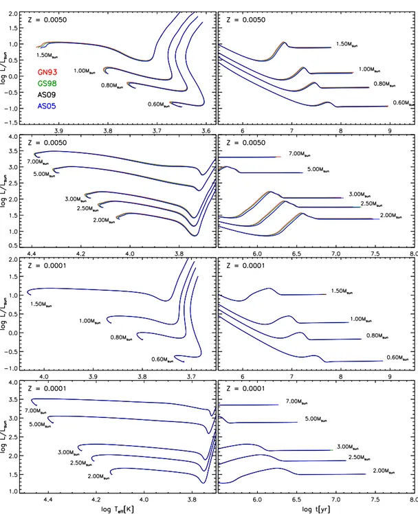
Figure 1.1: Comparison between non-grey models (BH05) with several masses in the range [0.01, 2.0] M⊙, computed adopting different τ values, namely τ = 2/3, 1, 10, and 100. Left panels: HR

diagram. Right panels: (log t[yr], R/R⊙) plane. A few specific evolutionary points, 1 Myr (filled

circle), 5 Myr (filled triangle), and 10 Myr (filled square) are also shown.

[M/H] value. I prefer this method because the atmospheric models generally ad-opts a chemical composition quite different from the one actually adopted for the interior computations, being different both the heavy elements mixture (metals abundances) and helium content. Thus, the interpolation at a fixed Z (which is independent of the choice made on the helium content and on the heavy element mixture) should be safer.

Another point to discuss is the choice of τ . As anticipated such value should be large enough to guarantee the diffusive approximation of the radiative transport to hold. This would lead to the choice of τ & 1. However, one has to notice that when a non-grey atmospheric model is adopted, the input physics used in the atmosphere are in general different from the one used for the interior of the star (i.e. the mixing length parameter, solar mixture, opacity. . .), so that a certain degree of inconsistency is always present. In order to limit this effect, large values of τ should be avoided (Montalb´an et al., 2004).

I recall that at this level the choice of τ is arbitrary, and once the two opposite requirements discussed above have been satisfied, all the choices are equally valid. I adopted the commonly used value of τ = 10 as the matching point between the interior and the atmosphere (see e.g., Morel et al., 1994). However, I checked the effect of a variation of τ on the track morphology in the HR diagram.

Figure 1.1 shows the effect of the adoption of a different value of τ in the range [2/3, 100] (keeping the atmosphere model constant to the BH05) for several masses, in the HR diagram (left panels) and in the (log t[yr], R/R⊙) plane (right

panels). It is evident that the choice of τ affects mainly the position of the star in the HR diagram through the effective temperature, leaving almost unchanged the luminosity at a given age.

The impact of τ on the track depends on both the mass and the evolutionary phase. Indeed, it is generally true that in case of radiative envelopes, the structure is almost independent of the adopted boundary conditions. On the contrary in the presence of thick convective envelopes the boundary conditions play a crucial role in determining the stellar radius, since the radiative loss efficiency is determined essentially by the properties of the most external atmospheric layers. This means that the Hayashi track of all the models and the ZAMS of low-MS stars (M . 1.0 M⊙) should be strongly sensitive to the different value of τ . This behaviour is well

reproduced for almost all the masses shown in Fig. 1.1, but not for M . 0.1 M⊙

when the stars contract towards the ZAMS. Such objects are so cold that electron degeneracy becomes progressively more and more important. Indeed, as I will show in the following (see Sect. 1.3.1), part of the structure of very-low mass stars lies in a region of partial electron degeneracy, thus their radius (and Teff)

is partially determined by the degeneracy level (pressure of degenerate electrons). This qualitatively explains why, as such stars contract towards low-temperatures, their effective temperatures are almost independent on the adoption of τ . I verified that for such objects even a variation of 10% of the pressure (or temperature) at the base of the atmosphere only marginally alters their position in the HR diagrams (a few percent in Teff).

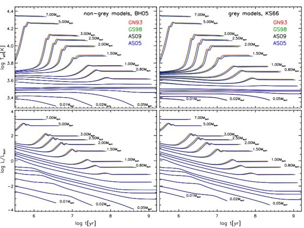
It can be worth to briefly discuss also how the adoption of different atmosphere models affects stellar evolution. Figure 1.2 shows the effect on the track position in the HR diagram of the use of the BH05, CK03, AHF11, and KS66 BCs, for several masses. Notice that, in the case of the CK03 models, very low-mass stars can not be computed since the minimum effective temperature available is Teff = 3500

K, which corresponds to about 0.5 M⊙ for the adopted chemical composition. In

order to make the comparison clearer, I show also some specific points of the stellar evolution, namely those corresponding to 1 Myr, 5 Myr, and 10 Myr. The boundary conditions used for the comparison are different among each other because of the adoption of several different input physics/parameters (EOS, opacity, mixing length value, chemical composition. . . ); so, it is reasonable to expect differences among the tracks computed adopting different BCs. However, it is not easy to disentangle the effect of each parameters (or physical input) from the others without a set of atmosphere models computed by possibly changing in turn only one parameter. Such calculations are unfortunately currently not available, and only qualitative speculations can be done.

Referring to Fig. 1.2, it is evident the large spread of the effective temperature at the same evolutionary phase for a fixed mass (see Table 1.2 and Table 1.3). For

Figure 1.2: Comparison in the HR diagram between models in the mass range [0.01, 2.0] M⊙,

computed adopting different boundary conditions; the non-grey BH05, CK03, and AHF11, and the grey KS66.The models corresponding to 1 Myr (filled circle), 5 Myr (filled triangle), and 10 Myr (filled square) are also shown.

M & 1.5 M⊙ (right panel) only the Hayashi line (and part of the Henyey track)

depends on the adopted BCs, whereas low- and very-low-mass models are strongly affected by the atmosphere models during most of their evolution. The largest differences occur, as expected, between the grey KS66 and the non-grey models in the case of low-mass stars, with differences in effective temperature as large as ∆Teff ≈ 230 K for M = 0.2 M⊙. I want to point out that the large differences in

Teff among the models occur where the stars have thick convective envelopes; such

differences could be partially reduced by changing the mixing length parameter, αML. Indeed, as I will discuss in the next section, such parameter plays a crucial

role in determining the effective temperature of a (non-adiabatic) convective star. Moreover, I will show that, if a solar calibrated αML is adopted (by fitting the Sun

radius), the differences in ZAMS between different BCs almost disappear for M & 0.6 M⊙.

As a final point, I want to show a comparison between the temperature-optical depth profile obtained from the KS66 and the one obtained from the BH05 model. The comparison is shown in Fig. 1.3 for several values of Teff, namely Teff =

2000, 3000, 4000, 5000, and 5700 (close to the solar Teff value): the BH05 models

corresponds to [M/H] = +0.0, for two surface gravities, namely log g = 3.0 and log g = 4.5, which are, respectively, representative of star close to the Hayashi track and to the MS. It is evident that large differences are present both for small and large values of τ . This is expected, since, as already stated, the KS66 T _{− τ is} not valid for the outermost atmosphere layers and for large values of τ . However,

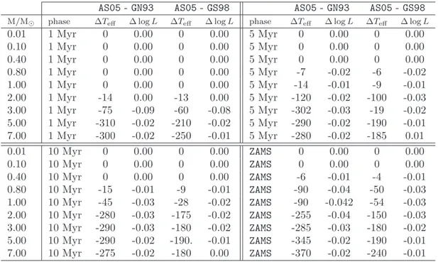
∆Teff

BH05-CK03 BH05-AHF11 BH05-KS66 M/M⊙ 1Myr 5Myr 10Myr 1Myr 5Myr 10Myr 1Myr 5Myr 10Myr

0.010 _{− − − −39 − − −77 − −} 0.050 _{− − −} 2 16 14 95 104 108 0.100 _{− − −} 29 20 18 127 153 164 0.200 _{− − −} 14 24 26 105 148 172 0.400 _{− − −} 64 30 25 114 127 143 0.600 29 109 125 73 62 46 109 138 146 0.800 29 64 81 125 67 68 116 138 150 1.000 35 55 64 96 108 157 122 141 159 1.500 52 92 137 106 141 209 148 208 356 2.000 68 214 −3 106 320 −2 177 561 2 ∆ log L/L⊙ BH05-CK03 BH05-AHF11 BH05-KS66 M/M⊙ 1Myr 5Myr 10Myr 1Myr 5Myr 10Myr 1Myr 5Myr 10Myr

0.010 _{− − − −0.01 − − −0.04 − −} 0.050 _{− − − −0.00} 0.00 0.00 0.03 0.00 0.01 0.100 _{− − −} 0.01 0.00 0.00 0.05 0.02 0.03 0.200 _{− − −} 0.00 0.01 0.01 0.02 0.03 0.04 0.400 − − − 0.00 0.00 0.00 0.01 0.02 0.03 0.600 0.00 0.03 0.03 0.00 0.01 0.00 0.01 0.03 0.03 0.800 0.00 0.02 0.02 0.02 0.00 0.01 0.01 0.02 0.03 1.000 0.00 0.01 0.01 0.01 0.02 0.03 0.01 0.02 0.03 1.500 0.00 0.02 0.01 0.01 0.03 0.02 0.02 0.04 0.04 2.000 0.01 0.02 0.00 0.01 0.03 0.00 0.02 0.06 0.00

Table 1.2: Differences in effective temperature (upper table) and luminosity (bottom table) between the non-grey reference set of models (BH05) and the CK03, AHF11, and KS66 ones, as shown in Fig. 1.2. The differences are given for the models corresponding to 1 Myr, 5 Myr, and 10 Myr.

there is an interval of τ values where the KS66 T_{− τ is quite close to the BH05 one:} 10−2 _{. τ . 5 for 4000 K . T}

eff . 5700 K and 10−1 . τ . 1 for 3000 K . Teff.

Notice also that for τ ≈ 1, the structures are only marginally affected by the different gravity. Thus, the use of a simple T _{− τ relation independent of g (just} like the KS66) is a quite reliable approximation for τ _{∼ 1. Large differences between} the two T−τ profiles are present for τ & 5 - 10, and in this case also surface gravity partially modifies the T_{−τ profile, especially in the case of cool objects. From this} comparison it emerges that the simple KS66 relation should be used for different Teff only in a limited range of τ (i.e. 0.1 . τ . 1); in particular, the adoption of

τ = 2/3 for the KS66 seems to be the best choice in the whole Teff range I analysed.

1.2.2

Convection

Pre-MSstars are, during their early evolutionary phases, cold and expanse objects. In such conditions, the matter becomes unstable for convective motions in almost

ZAMS

BH05-CK03 BH05-AHF11 BH05-KS66 M/M⊙ ∆Teff ∆ log L/L⊙ ∆Teff ∆ log L/L⊙ ∆Teff ∆ log L/L⊙

0.010 − − − − − − 0.050 − − − − − − 0.100 − − 15 0.01 97 0.04 0.200 − − 30 0.01 229 0.10 0.400 − − 28 0.01 165 0.06 0.600 26 0.00 35 0.01 91 0.01 0.800 13 0.00 51 0.00 79 0.01 1.000 51 0.00 60 0.00 138 0.00 1.500 0 0.00 0 0.00 2 0.00 2.000 1 0.00 5 0.00 13 0.00

Table 1.3: Differences in effective temperature and luminosity between the non-grey reference set of models (BH05) and the CK03, AHF11, and KS66 ones, as shown in Fig. 1.2, for the ZAMS models.

all the structure, so that convection becomes the main source of heat transport towards the stellar surface. Moreover, depending on the mass and chemical com-position, convective envelopes are present also as the star approaches the ZAMS. Thus, the treatment of convective heat transport plays a crucial role in determin-ing the characteristic of pre-MS stars.

A complete and detailed method to describe convection in stars should relies on hydrodynamical simulations of turbulent fluids. Such simulations have been par-tially carried out in recent years, but only for small fraction of the stellar structure, and never for the computation of a complete stellar evolutionary sequence, essen-tially because the computational complexity that the simulations require (see e.g., Nordlund, 1982; Freytag et al., 2002; Ludwig et al., 2002; Collet et al., 2007; Beeck et al., 2012, and references therein). Given this situation a much more simplified approach to solve the problem is commonly adopted, through mono-dimensional and time-independent formalisms.

The most largely used convection treatment is the Mixing Length Theory (MLT), which relies on the formulation proposed by B¨ohm-Vitense (1958). In this form-alism, convection is treated as two columns of matter, one hot that is rising and the other cold that is sinking, so that the total flux of matter is zero. The heat transported by the hot rising matter is released as the gas mixes with the sur-rounding environment. The mean path travelled by the upward moving matter (mixing length) can not be obtained a priori in this scheme but it is assumed to be a multiple of the pressure (or density) length scale, thus it is given by (using the pressure scale Hp),

ℓ = αMLHp (1.12)

where αMLis a free parameter (mixing length parameter ). I want to emphasize that

Figure 1.3: Comparison between the T−τ profile obtained from the grey KS66 and the non-grey BH05atmospheric models. The comparison is shown for different effective temperatures (Teff =

2000, 3000, 4000, 5000, and 5700 K). In the case of BH05 two gravity values (log g[cms−2_{] = 3.0}

and 4.5) representative of Hayashi track and ZAMS models are also shown.

it completely neglects the spectral distributions of the turbulent eddies, which defines the dimensions of convective cells. Convective cells are supposed to have an averaged dimension given by ℓ.

Within the MLT formalism, the temperature gradient actually present in a region of the star (∇ ≡ ∂ log T/∂ log P ) can be obtained by solving the following cubic equation (see e.g. Cox & Giuli, 1968),

ξ1/3+ Bξ2/3+ a0B2ξ− a0B2 = 0 (1.13)

ξ def= ∇rad− ∇ ∇rad− ∇ad

(1.14) where a0 ≡ 9/4 is a geometrical factor, ∇ad, and ∇rad are, respectively, the

adia-batic and radiative gradients, and B is a coefficient that depends on the difference between the radiative3 _{and adiabatic gradient and on the ratio between the}

con-vective and radiative conductivity. It is interesting to write explicitly B in order to underline its dependency on several physical quantities, such as the temperature T , pressure P , gravity g, and in particular on the opacity of the gas (Rosseland mean opacity, κR) and on the quantities obtained from the equation of state (density ρ,

3

specific heat cP, adiabatic gradient, molecular weight µ, and their derivatives), B def= hA 2 a0 (_∇rad− ∇ad) i1/3 (1.15) A def= r QρP3 2 cPκR 48σsbgT3 α2_ML (1.16) Q def= −∂ log ρ ∂ log T    µ, P − ∂ log ρ ∂ log µ    T ∂ log µ ∂ log T    P (1.17)

Once eq. (1.13) has been solved, the temperature gradient in the star is given by the relation,

∇ = (1 − ξ)∇rad+ ξ∇ad (1.18)

Since ξ ∈ [0, 1], it results that in the case of convective regions, the temperature gradient is forced to lies between the adiabatic and radiative one, i.e. _∇ad .∇ .

∇rad. The two limiting cases correspond to high convection efficiency (ξ ≈ 1,

∇ ≈ ∇ad) and low convection efficiency (ξ ≈ 0, ∇ ≈ ∇rad). It is useful to define

also the super-adiabaticity, _{∇ − ∇}ad, as the difference between the real and the

adiabatic gradient.

The value of ∇ is strongly correlated to the physical conditions of the region considered, and it can varies abruptly inside a star depending on its mass. In order to investigate in a more quantitative way the dependency of_{∇ on the various} quantities given in eqs. (1.15) - (1.17), I considered three points along the evolution of a pre-MS stars, namely a cold and expanse structure at the beginning of the Hayashi track, the point at the age of 1 Myr, and the ZAMS model, for stars of 0.01, 0.1, 1.0, and 7.0 M⊙. Figure 1.4 shows the profile along the entire structure

of _{∇(thick grey line) and ∇}ad (dashed black line) at such selected points. With

the purpose of making a sensitivity analysis, hence to show the dependence of _∇ on the coefficients (κ, cP, ∇ad, and αML) in eqs. (1.15) - (1.17) in different masses

and/or evolutionary phases, I evaluated the effect of changing of 10%, separately, κR, cP,∇ad, and αML, by keeping fixed the temperature and pressure in each mass

shell to their original (reference) values. Thus, I computed the relative difference between the new _{∇ value obtained solving eq. (1.13) and the reference one.}

First of all it is evident that in the case of very low-mass stars (M . 0.1 M⊙),

∇ ≈ ∇ad in the whole structure. Due to the large densities involved, even a

small super-adiabaticity guarantees the required amount of heat transported by convection (Q = CP∆T ∝ ρcP∇). When this happens, ∇ is determined essentially

by the EOS through ∇ad and it is independent of the other quantities. As the star

mass increases, the structure gets progressively less dense (e.g. for M = 1 M⊙). The

interior are still adiabatic, while in the envelope the situation is different depending on the evolutionary phase. In the first evolution along the Hayashi track it is sensitively over-adiabatic. However, as the structure contracts, the region where ∇ > ∇ad withdraws towards the most external layers. In all the regions where

Figure 1.4: Profile of the temperature gradient_{∇ (thick-grey solid line) and the corresponding} value of∇ad(thick-black dashed line) along the whole structure of models with different masses

(M = 0.01, 0.10, 1.0, and 2.0 M⊙) at the beginning of the Hayashi track (left panels), at the age

of 1 Myr (central panel ), and for the ZAMS (right panels). The relative difference between the actual value of_{∇ and the one obtained if κ}R, ∇ad, cP, and αML are changed by ±10% in each

Figure 1.5: Effect on the tracks position in the HR diagram of the adoption of two different values of the mixing length parameter, namely αML= 1.68 (reference value) and αML= 1.00 for

stars in the mass range [0.01, 2.0] M⊙. The models corresponding to 1 Myr, 5 Myr, and 10 Myr

are also shown.

Notice that for M = 1 M⊙the inner region are radiative, so,∇ = ∇rad <∇ad; in this

case _{∇ ∝ κ}R. For larger masses (M & 1 M⊙) the temperature gradient evolves in a

different way. After the evolution along the Hayashi track (fully convective star), the structure arrives in ZAMS with a convective (adiabatic) core and a radiative envelope. The temperature gradient in the envelope depends only on the opacity and not on αML.

In order to emphasize the dependency of the models on αML, I show in Fig. 1.5

two sets of tracks computed adopting αML = 1.0 and 1.68. From the discussion

above it should be easy to understand the different effect of αML on different

evolutionary phases. In particular it is evident that for M . 0.4 M⊙ only the first

evolution along the Hayashi track depends on αML. In the interval 0.6 . M/M⊙ .

1.0 the whole evolution up to the ZAMS depends on the mixing length parameter, while for M & 1.5 M⊙ the ZAMS is completely unaffected by the choice of αML.

It can be worth to quantify also the effect of the adoption of different αML on

the age and mass determination, given a point in the HR diagram. I show in Fig. 1.6 a set of models computed with αML = 1.68 in the mass range (0.6 - 1.0 M⊙)

with over imposed a 0.8 M⊙ and 1.0 M⊙ track with αML = 1.0. I also show the

points where the αML = 1.0 tracks achieve the same luminosity and temperature

of the αML = 1.68 models. It is evident that the same position in the HR diagram

can be obtained with different masses and ages, as shown in Table 1.4. Notice the large differences both in ages (about 30 - 40% after 1 Myr), and in mass (about 0.2 M⊙).

From the previous example it turns out the importance of using a suitable value of αML. Thus, it can be useful to discuss the choice of αML, which, as already

Figure 1.6: Effect of the adoption of two values of αMLon the mass determination for a given

luminosity and effective temperature in the HR diagram for models with αML= 1.68 (blue-dotted

line, M = 0.6 - 1.0 M⊙) and αML= 1.00 (red-solid line, M=0.8 and 1.0 M⊙). The points where

αML= 1.00 and αML = 1.68 models achieve the same log L/L⊙and log Teff are shown too (black

circles). M/M⊙ point M/M⊙ ∆t[yr]/t[yr] (αML = 1.00) (αML= 1.68) 0.8 a 0.6 +45% b 0.7 +29% c 0.8 +25% 1.0 d 0.7 +53% e 0.8 +37% f 0.9 +43% g 1.0 +39%

Table 1.4: Age and mass difference for the models shown in Fig. 1.6 (αML = 1.00 and 1.68)

at the labelled points in the HR diagram. The age difference is defined as ∆t[yr] = tα 1.00[yr]−

tα 1.68[yr].

techniques that can be followed: 1) MS or RGB4 _{(red-giant branch) calibration and}

2) solar calibration.

In the first case, a direct comparison between theoretical models and observed cluster stars colour is performed. One possibility is to obtain the most suitable mixing length parameter by imposing to reproduce the color of the part of the MS

populated by stars with convective envelopes. This correspond approximatively to the mass interval 0.6 . M/M⊙ .1.2, for solar metallicity stars. Indeed, for higher

masses the convective envelope disappears, while for M . 0.6 M⊙ the convection

becomes essentially adiabatic and does not depend on the choice of αML (see Fig.

1.4). Another possibility is to compare models with observed RG stars in the CMD5_.

Such stars have thick and expanse convective envelopes and populate a region almost vertical in the CMD, thus their color index6 _{strongly depends on α}

ML. Of

course this method can be applied only if red giant branch is actually present and if it is populated by a large sample of stars (e.g. globular clusters).

A completely different method consists in fitting the solar radius. Indeed, the Sun has a convective envelope that extends down to about 0.7 R⊙ (Rbce/R⊙ =

0.713± 0.001, see e.g., Basu & Antia, 1997), which makes the solar radius (ob-tained from stellar evolution computation) sensitive to the adopted mixing length parameter. I performed the calibration of αML,⊙ by computing a standard solar

model with PROSECCO. It consists in a 1 M⊙model that at the age of 4.57 Gyr must

reproduce the surface observables of the Sun, which are the luminosity, radius, and (Z/X)surf,⊙, within a given tolerance (∆ log L/L⊙ ≤ 10−5, ∆R/R⊙ ≤ 10−4, and

∆(Z/X)surf/(Z/X)surf,⊙ ≤ 4×10−4). For (Z/X)surf,⊙ I adopted the recent

determ-ination by Asplund et al. (2005) (see Section 1.3.3).

As shown in the previous section, the adoption of different BCs affect the position of 1 M⊙ in ZAMS; the solar model is affected too. To this regard I computed solar

models for the aforementioned boundary conditions, namely BH05, CK03, AHF11, and KS66. The resulting evolutionary tracks corresponding to the solar model are shown in Fig. 1.7. The main effect of the BC is to shift the effective temperature; so, it is expected that different αML values are required to reproduce the position

of the Sun in the HR diagram if different BCs are adopted.

The models with different BCs are constructed to reproduce the position of the Sun in the HR diagram, so the corresponding ZAMS are very close. However, the solar calibration does not assure the Hayashi tracks to be similar. Indeed, the differences in effective temperature among models computed with different BCs/αMLare clearly

visible in Fig. 1.7. The largest discrepancy occurs between the KS66 and AHF11 at about 1 Myr (∆Teff ≈ 90 - 100 K). Notice also that the four models tend to

converge at the base of the Hayashi track (_{∼ 10 Myr), when the model develops} a radiative core. Indeed, the effective temperature differences decreases rapidly to about ∆Teff ≈ 50 K at the age of 10 Myr. Only the AHF11 model shows a peculiar

behaviour, being in this point the more distant from the other.

I want to emphasize also that the adoption of a solar calibrated value of αML

helps to reduce the differences in effective temperature near the ZAMS of models with (non adiabatic) convective envelopes computed using different boundary conditions (i.e. 0.6 . M/M⊙.1.2).

5_{CMDstands for Colour-Magnitude Diagram.}

6_{The color index is the difference between the star magnitudes in two different photometric}

Figure 1.7: Comparison between 1 M⊙ tracks computed adopting the solar calibrated value of

αML as obtained from the adoption of the BH05, CK03, AHF11, and KS66 boundary conditions.

The models corresponding to 1 Myr (filled-circle), 5 Myr (filled-triangle), 10 Myr (filled-square) and the position of the Sun (⊙) are also shown.

As a concluding remark, it is worth to notice that, however obtained, the calib-rated mixing length parameter is then used also for stars with different masses and in different evolutionary phases. Although this is a commonly adopted procedure, one has to pay attention to use the calibrated αMLalso for other stars. Indeed, there

is no reason to assume αMLto be the same independently of the mass, evolutionary

phase, and/or chemical composition. On the contrary, there are hints of a possible dependence of αML on the mass effective temperature and gravity, as suggested by

observations (see e.g., Chieffi et al., 1995; Morel et al., 2000; Ferraro et al., 2006; Yıldız, 2007; Piau et al., 2011; Bonaca et al., 2012) or detailed hydrodynamical simulations (see e.g., Ludwig et al., 1999; Trampedach, 2007). Moreover, many authors as already pointed out the necessity of a lower convection efficiency with respect to the solar calibrated one to reproduce the observed radius of pre-MS binary systems (see e.g., Mathieu et al., 2007; Gennaro et al., 2012, and references therein and Chapter 2): these comparisons seem to privilege αML ∼ 1. Such a

low-αMLvalue is suggested also by the analysis of surface7Li abundances in young

1.3

Micro-physics

1.3.1

Equation of state

The Equation Of State (EOS) supplies all the thermodynamical quantities required for the integration of a stellar structure. During their evolution, stars with different masses span a wide range of temperatures and densities, therefore, in order to compute stellar models, it is necessary the use of an accurate EOS for the whole range of temperature and densities covered by the calculations. The accuracy of the EOS becomes particularly important in low-mass and cold models, due to the role played by partial ionization, pressure ionization and dissociation. A detailed treatment of the partially ionized regimes is very important since it affects the extension of the convective envelope and, concerning pre-MS models, the shape of the tracks, where the model leaves the Hayashi track and move towards higher effective temperatures (D’Antona, 1993). In the case of high density, the EOS must account for many non ideal effects, not least the ionization pressure and dissociation (e.g. Saumon et al., 1995). In addition, in low-mass stars the convective transport is almost adiabatic even in the outer envelope, due to the high density of matter (see discussion in Sect. 1.2.2). In this case the effective temperature and the radius are essentially determined by the adiabatic gradient provided by the EOS.

In the last 20 - 30 years, several EOS have been developed for stellar compu-tations. The principal difference among the EOS relies on the scheme adopted to describe the matter in stellar condition. Generally two different schemes are adop-ted: the physical and the chemical picture (see e.g., Trampedach et al., 2006). In the former, the electrons and nuclei are considered as the fundamental constitu-ents of the gas, which interact themselves through the coulombian potential. A complete description of the gas of interacting particles is then achieved by solving the Schroedinger equation for a many-body system, providing the bound states (atoms, ions and molecules) and the free electron states. The advantage of this approach is to solve simultaneously both the statistical and quantum problem, giv-ing thus a complete and rigorous treatment of the gas. However, a disadvantage is the numerical and computational complexity of the method, which can be hardly applied to high-density low-temperature regimes. Nevertheless, this method has been successfully applied to compute the OPAL EOS (Rogers et al., 1996; Rogers & Nayfonov, 2002) in a very wide range of temperature and density suitable to model stars greater than about 0.1 M⊙ (the exact value depending on the chemical

composition and on the evolutionary phase).

A more simple way to obtain a description of the gas is based on the chemical picture. In this case, atoms, molecules, and ions are the fundamental particles which interact through pair-potentials. Given the description of the gas, the solu-tion is achieved first by solving the quantum problem and then by populating the states via statistical mechanics. The method consists in computing the free energy as a function of temperature, density and species number. Then, the equilibrium is obtained by minimising the free energy. This gives the equilibrium

concentra-EOS definition units

T temperature K

P total pressure erg cm−3

ρ density gr cm−3

cP specific heat at constant P erg gr−1 K−1

∇ad adiabatic gradient

-µ mean molecular weight

-Γ1 ∂ log P/∂ log ρ|S

-χρ ∂ log P/∂ log ρ|T

-χT ∂ log P/∂ log T|ρ

-Table 1.5: Thermodynamic quantities used in the FRANEC code.

tion of each specie and by deriving the free energy also all the thermodynamical quantities. This technique has several advantages with respect to the physical pic-ture, being computationally less complex and giving the possibility to be applied to high-density and low-temperature regimes, which, at present, are not covered in the physical picture. A disadvantage is the need for ad hoc pair-potential, pres-sure ionization, and non-ideal effects, for the interacting species, which has to be introduced in an heuristic way. Examples of still largely used EOS computed in the chemical picture are FreeEOS (Irwin, 2004), the MHD (Hummer & Mihalas, 1988; Mihalas et al., 1988; Daeppen et al., 1988), the PTEH (Pols et al., 1995) and the SCVH95 (Saumon et al., 1995), the latter being widely used for the computations of low- and very-low-mass stars.

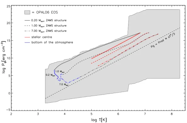
Given the complexity of the EOS computation, generally, the EOS is supplied to the evolutionary code as pre-computed tables to be interpolated. The models I discuss in this PhD work have been mainly computed by adopting the most recent version of the OPAL EOS7_{, released in 2006 (OPAL06), which at present is the most}

reliable, accurate, and complete equation of state available. As anticipated above, such an EOS is available in a wide temperature range, i.e. 1870 K_{≤ T ≤ 2 × 10}8_K,

and pressure range, −3 ≤ log Pg[erg cm−3] ≤ 24 depending on T . The validity

range of the OPAL06 EOS is shown in Fig. 1.8, where I plotted also the evolution of the centre (thick red line) and of the bottom of the atmosphere (thick blue line) for models with different masses (0.2, 1.0 and 7.0 M⊙) from the early pre-MS to

the ZAMS phase. The entire structure for the ZAMS models are shown, too.

The OPAL06 EOS is released as tables that contain the thermodynamical quant-ities of the gas, i.e. without the contribution of the radiation, computed for several temperatures, chemical compositions, and densities. The tables are available for a mixture of hydrogen (X), helium (Y ) and metals, namely 5 hydrogen abundances X = 0.0, 0.2, 0.4, 0.6, 0.8 and 3 metallicities Z = 0.00, 0.02, 0.04.

In order to use the EOS in the evolutionary code, the OPAL06 tables have to be converted in a suitable format and the contribution of the radiation to the

Figure 1.8: Validity domain of the OPAL06 EOS (shaded area) in the (log T , log Pg) plane with

over plotted the temporal evolution of the bottom of the atmosphere (τph=10, thick blue line)

and the stellar centre (thick red line) for 0.2, 1.0, and 7 M⊙. The whole structure for the ZAMS

models are also shown.

dynamical quantities has to be added. First of all I used as independent quantities the temperature (T ) and the gas pressure (Pg). I built new EOS tables interpolating

the OPAL06 EOS (pure gas) on a finer grid of pressure, spaced by ∆ log P = 0.05. This step helps to avoid the introduction of additional errors coming from the EOS interpolation inside the evolutionary code. The second step consists in adding the contribution of the radiation, and computing all the thermodynamical quantities needed (see Table 1.5). This procedure is described in detail in Appendix A.1

Once the tables containing gas plus radiation have been developed, a further interpolation of the EOS at the required value of the initial metallicity Z of the star has been performed. In conclusion the EOS table provided to the code contains the thermodynamical quantities computed for 5 hydrogen abundances, for several value of Pg and T (to be interpolated in the code) for a given Z. To this regard,

it is worth noticing that the metallicity changes during the star evolution because of nuclear burning and/or diffusion/mixing. However, during the pre-MS and MS phases it is generally accepted to adopt an EOS with a constant value of Z, i.e. equal to the initial metallicity used for the star. The reason to proceed in this way is the negligible dependency of the equation of state on the metallicity. I checked this statement computing the EOS for two different Z values, Z = 0.02 and Z = 0.00. I found that the thermodynamical quantities used in the code are

quite insensitive to the adopted Z, showing discrepancies of less than 2 - 3 % (see also Chabrier & Baraffe, 1997). Consequently, due to the small dependency on Z and the large computational time that would be required to re-compute the EOS for each value of Z, I followed the common approach of neglecting the changes in Z in the EOS.

As clearly visible from Fig. 1.8, the OPAL06 EOS does not cover the entire parameter space required to compute the evolution of very-low mass stars, i.e. M .0.1 M⊙. Indeed, referring to the figure, the ZAMS structure of a 0.2 M⊙ is barely

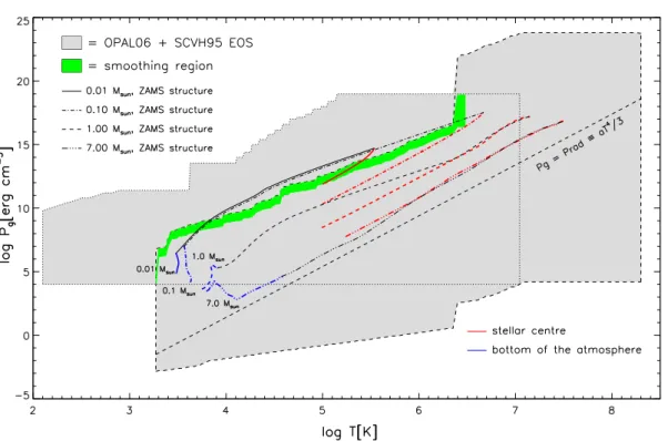
enclosed inside the OPAL06 ranges. This is a limitation of such an EOS. In order to overcome this problem, I extended the EOS tables by means of the SCVH95 EOS (Saumon et al., 1995). Such an EOS is largely used for the computation of very-low mass stars, brown dwarfs, and planetary models, being able to reach very-very-low temperatures (few hundreds of kelvin) and relatively high densities.

The SCVH95 EOS consists of pure hydrogen and pure helium tables without the inclusions of metals; however, as already stated, the lack of metals in the EOS only marginally affects the thermodynamic quantities (during pre-MS and MS) and it can be neglected. The SCVH95 EOS accounts for molecular, neutral, and ionized hydro-gen (H2, H, and H+), plus free electrons coming from the hydrogen ionization, and

neutral, and ionized helium (He, He+_{, and He}2+_{), plus helium ionization electrons.}

The interaction between helium and hydrogen species is not considered at this stage of the EOS computation8_{. The SCVH95 EOS is available in a temperature range}

log T [K]_{∈ [2.10, 7.06], which roughly corresponds to 126 K . T . 1.14×10}7_{K, and}

4≤ log Pg[erg cm−3]≤ 19, the pressure upper limit depending on the temperature.

Radiation is not included in the available tables.

With the aim of extending the OPAL06 EOS, the SCVH95 original tables have been interpolated on the OPAL06 grid of temperature and pressure in those region where the two EOS overlap, i.e. 1870 K_{≤ T ≤ 1.14 × 10}7_{K. Out of this region the}

SCVH95 (T < 1870 K) and the OPAL06 (T > 1.14× 107 _{K) temperature grid has}

been, respectively, adopted. The pressure grid spacing is kept fixed to ∆ log P = 0.05 even for the SCVH95 EOS.

The construction of the SCVH95 EOS tables requires a different method with respect to the construction of the OPAL06 ones, because the latter one is available for a mixture of hydrogen and helium, while the former not. Hence, the pure hydrogen and pure helium SCVH95 tables have to be combined in order to obtain the same mixture of H and He used for the OPAL06. This has been done adopting the additive-volume rule (for more details see Appendix A.1). This method relies on the assumption that extensive quantities like volume, mass, energy, entropy, particles number, etc. . . are additive when two or more particles systems are combined together. On the contrary, temperature and pressure do not change if such systems, in equilibrium, are merged (intensive variables). These assumptions are exactly true for ideal, identical, and non-interacting particles, while they are only an approximation for real systems. However, this method has been largely 8_{The mixing of H and He species is accounted for in the mixing entropy (see Appendix A.1).}