Theoretical and experimental analysis of microwave heating processes

(1)

UNIVERSITY OF SALERNO

DEPARTMENT OF INDUSTRIAL ENGINEERING

Ph. D. Thesis in Mechanical Engineering

XIIICYCLEN.S.(2011-2014)

“Theoretical and experimental analysis of

microwave heating processes”

Laura Giordano

Supervisor Coordinator

Ch.mo Prof. Ing. Ch.mo. Prof. Ing. Gennaro Cuccurullo Vincenzo Sergi

(2)

(3)

Alla mia famiglia e a tutte le persone che mi vogliono bene

(4)

(5)

I

NDEX OF FIGURES

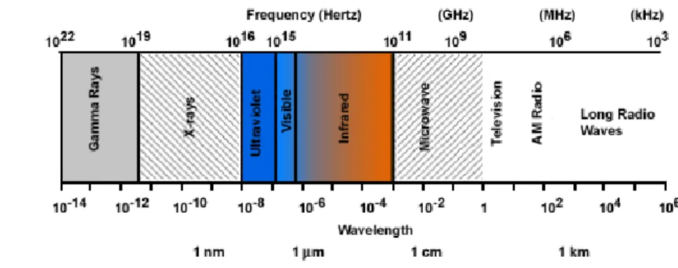
Figure 1.1 Electromagnetic spectrum ... 7

Figure 1.2 Electromagnetic wave propagation ... 7

Figure 1.3 Dielectric permittivity of water ... 16

Figure 2.1 Microwave pilot plant heating system ... 18

Figure 2.2 Real-time IR thermography for apple slices ... 19

Figure 2.3 Temperature fluctuations for the selected temperature levels 19 Figure 2.4 Drying curves of apple slices by hot air (dashed line) and microwave (continuous line) heating at 55, 65 and 75 °C. ... 22

Figure 2.5 Drying rate curves ... 22

Figure 2.6 Sample geometry ... 25

Figure 2.7 Analytical prediction (continuous lines) vs experimental trend (falling rate period) ... 27

Figure 3.1 Scheme of the single mode cavity ... 31

Figure 3.2 Modulus of the “z-component” of the electric field ... 31

Figure 3.3 Modulus of the “x-component” of the electric field ... 31

Figure 3.4 Bi-dimensional map of the electric field norm ... 32

Figure 3.5 Scheme of the experimental setup ... 33

Figure 3.6 Experimental set-up ... 33

Figure 3.7 The thermoformed tray ... 35

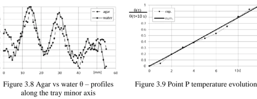
Figure 3.8 Agar vs water θ – profiles along the tray minor axis ... 36

Figure 3.9 Point P temperature evolution ... 36

Figure 4.1 Sketch of the avaiable experimental set-up ... 42

Figure 4.2 Temperature variations of water along the axis of the pipe .... 46

Figure 4.3 RMSE calculated with respect to the reference solution characterized by the maximum sampling density ... 46

Figure 4.4 Contour plots and longitudinal distributions of specific heat generation Ugen along three longitudinal axes corresponding to the points, O (tube centre), A, B. ... 52

Figure 4.5 Cross sections, equally spaced along the X-axis, of temperature spatial distribution ... 53

(8)

Figure 4.7 Temperature radial profiles... 55

Figure 5.1 Flowchart of the assumed procedure ... 57

Figure 5.2 Dielectric constant, ’ ... 60

Figure 5.3 Relative dielectric loss, '' ... 60

Figure 5.4 Heat generation along the X axis for Uav = 0.08 m/s ... 61

Figure 5.5 Interpolating function (green line) of the EH heat generation distribution (discrete points) for Uav = 0.08 m/s ... 63

Figure 5.6 Bulk temperature evolution for Uav = 0.008 m/s ... 66

Figure 5.7 Bulk temperature evolution for Uav = 0.02 m/s ... 66

Figure 5.8 Bulk temperature evolution for Uav = 0.04 m/s... 66

Figure 5.9 Bulk temperature evolution for Uav = 0.08 m/s... 66

Figure 5.10 Spatial evolution of the error on the bulk temperature prediction... 67

Figure 5.11 Root mean square error with respect to the CN solution ... 68

Figure 6.1 Planck’s curves plotted on semi-log scales ... 71

Figure 6.2 Schematic representation of the general thermographic measurement situation ... 73

Figure 6.3 Sketch and picture of the available MW pilot plant ... 76

Figure 6.4 Net apparent applicator pipe temperatures ... 79

Figure 6.5 Effective transmissivity for the selected temperature levels .. 80

Figure 6.6 Measured and interpolated relative shape-function f1... 80

Figure 6.7 Temperature level function f2 obtained with a linear regression ... 80

Figure 6.8 The reconstructed and measured true temperature profiles @ Tinlet = 55°C ... 80

Figure 6.9 Theoretical and experimental bulk temperatures for inlet temperatures Tinlet= 40, 45 and 50 °C, and two flow rates m = 3.2 and 5.4 g/s. ... 83

(9)

I

NDEX OF TABLES

Table 2.1 Set temperatures, averages, temperature oscillations and standard deviations (SD) during ﬁrst and second half of drying time by

microwave of apple slices. ... 21

Table 2.2 Data reduction results ... 28

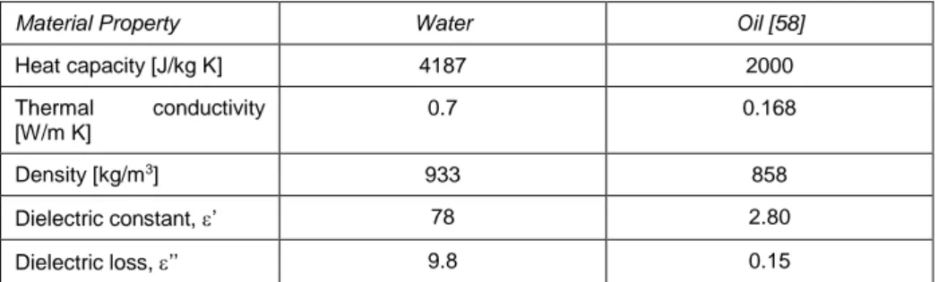
Table 3.1 Oil and water properties ... 37

Table 3.2 H-configuration ... 38

Table 3.3 V-configuration ... 39

Table 4.1 Dimensionless partial problems: uniform heat generation solution ... 50

Table 5.1 Dimensionless partial problems: BH and EH hybrid solutions 64 Table 5.2 Computational time for CN and BH solutions ... 68

Table 6.1 RMSE of bulk temperatures for different mass flow rates and temperature levels ... 82

(10)

(11)

INTRODUCTION

Thermal processing is the major processing technology in the food industry and its purpose is to extend the shelf life of food products without compromising food safety. Apart from the positive effect of food treatments, such as the inactivation of pathogens, there are also some limitation by way of partial destruction of quality attributes of products, especially heat-labile nutrients, and sensory attributes.

The technological revolution, nutritional awareness, and continuous demand of the new generation have necessitated search for new or improved food processing technologies. Presently, several new food processing technologies, including microwave heating, are investigated to improve, replace, or complement conventional processing technology. Microwave has been successfully used to heat, dry, and sterilize many food products. Compared with conventional methods, microwave processing offers the following advantages: 1) microwave penetrates inside the food materials and, therefore, cooking takes place throughout the whole volume of food internally and rapidly, which significantly reduces the processing time; 2) since heat transfer is fast, nutrients and vitamins contents, as well as flavor, sensory characteristics, and color of food are well preserved; 3) ultrafast pasteurization or sterilization of pumpable fluids minimizes nutrient, color, and flavor losses; 4) minimum fouling depositions, because of the elimination of the hot heat transfer surfaces, since the piping used is microwave transparent and remains relatively cooler than the product; 5) energy saving because of the absence of a medium between the sample and the MW; in addition, if the system is well projected, high efficiency can be reached (some authors showed the reduction of the energy costs during drying processes using microwaves, with a further improvement using air dryer and microwaves in sequence [1]; moreover, consider the possibility to use alternative energy sources, eg. photovoltaic); 6) perfect geometry for clean-in-place system; 7) low cost in system maintenance; 8) space saving, if the system is compared with the traditional ones, based on boilers and surface heat exchangers [2].

On the other hand, there are some problems which prevent the diffusion of this technique; among them: 1) uneven temperature patterns of the food processed, due to the uneven temperature field inside the microwave

(12)

cavity; 2) temperature readout and control problems, because traditional probes fail: in particular, the thermocouples disturb the measurement and are damaged by the electric field, while fiberoptic probes allow to know the temperature only in few points; 3) difficulties in predicting the temperature field, because of coupling of three physical phenomena, that is, electromagnetic wave propagations, heat transfer and, in most of cases, fluid motion. Consider that sizing, during the design phase, and the control, during the operating phase, could be based on theoretical predictions, avoiding the so called “trial and error” approach.

To address the critical points mentioned above, during the thesis work, theoretical models were developed and experimental tests were performed, with reference to “batch” and “continuous flow” processes. Batch processes and related models are described in the former part of this thesis and encompass both apple drying and in package-processes of water and oil. The second part deals with continuous processes which are more interesting, having in mind industrial applications.

Drying processes

Drying is a thermal process, because the saturation pressure increases with temperature; as a consequence, the drying rate is related to the

temperature level. This technique is widely used for food preservation,

but long drying times and high temperatures are required by using sunlight or conventional hot air drying. Conventional drying turns out to be a low efficient process because of the foods low thermal conductivity and high internal resistance to moisture transfer [3-34]. Thus an increasing demand for faster procedures is arising in the food industry. In this connection, microwave (MW) driven drying processes have been studied extensively in the last decade since it is well known that they provide an efficient mean for moisture removal. In facts, it has been demonstrated that, for a large variety of foods, microwave heating considerably lowers drying times without damaging flavour, colour, nutrients of the fruit [4-11; 19;22]. Improved drying rates can be explained considering that the interior of the sample is quickly heated by internal heat generation due to MW exposition and, as a consequence, the generated vapour is forced towards the surface where it is easily removed by the air flow. Furthermore, fast vapour expulsion creates a porous structure which facilitates the transport of vapour being responsible of reduced shrinkage [12-14;20].

(13)

Introduction 3 As a matter of facts, typically, drying processes are carried-on fixing power rather than temperature levels: this occurrence can lead to product overheating, with charring and unacceptable final quality [17;20;39-41; 46]. Thus, it is clear that temperature must be controlled [40-44] but such procedure is seldom reported in the literature [45-46], probably for the reasons outlined before.

The problems underlined above about the uneven temperature patterns and the difficulties in measuring and controlling the food temperature will be addressed by showing a new microwave drying system which allows to control the product temperature acting on the magnetron duty cycle. In particular, the temperature was controlled looking inside the MW chamber by an IR equipment, thus obtaining thermal maps with high resolution.

Drying kinetics will be analysed through the determination of the effective mass diffusivity by applying a 2D unsteady analytical model.

In-package processing of liquids

The second batch application addressed in this thesis, the in-package processing, has recently determined a growing interest in using new packaging materials-dielectric and/or magnetic-in a wide variety of applications for controlling the microwave heating of food. Packaging materials need to be microwave transparent and have a high melting point, with shapes adapted for microwave heating [47].

Wishing to perform in-package pasteurization or sterilization, there is to face the uneven temperature distribution, which determines both the magnitude of time-temperature history and the location of the cold points as functions of the composition (ionic content, moisture, density, and specific heat), shape, and size of the food [48-52;58;72], for a given equipment. In fact, unlike conventional heating, the design of the equipment can more dramatically influence the critical process parameter: the location and temperature of the coldest point. Many variables such as dielectric properties, size, geometry and arrangement of food materials affect the heating uniformity, the latter being a critical matter. It then follows that the potential application of these techniques requires an

accurate study of the thermal patterns of the food. The uneven

temperature field in the samples can be improved by acting both on the illuminating system and on target food. In particular, thermal response for water and oil samples, placed in a special thermoformed tray, with

(14)

different size and orientation will be studied. The first aim will be to show that temperature predictions, obtained by a commercial numerical software based on Finite Element Method (FEM), can recover experimental results. Then, uniformity in temperature distribution will be investigated both through the numerical FEM runs and the corresponding experimental tests in a pilot plant.

Continuous flow microwave heating of liquids

The second part of the work deals with the continuous flow microwave heating processes, above mentioned; this systems, respect with the batch ones, are featured by increased productivity, easier clean up, and automation. Several laboratory-based continuous-flow microwave heating systems have been used for fluid foods with different configurations [53-57]. Nowadays, the numerical approach allows a quite satisfying description of the coupled thermal-EM problems as well as an accurate identification of the effects which the operating parameters have on the process at hand [54;65-68;71-72;75-76], provided that spatial discretization is performed with care as grid dispersion may arise [74]. Starting from the pioneering work of Yee [77] in which Maxwell’s equations were solved with a primitive 2D version of the Finite Difference Time Domain (FDTD) technique, remarkable contributions have been given so far. Zhang et al. [68] proposed a 3D FDTD model to describe electromagnetic field patterns, power temperature and velocity distributions in a confined liquid inside a microwave cavity. Chatterjee et al. [78] numerically analyzed the effects on the temperature distribution of a liquid in terms of the rotating container, natural convection, power sources and shape of the container. Zhu et al. [79] developed a more sophisticated procedure to solve cases with temperature-dependent dielectric permittivity and non-Newtonian liquids carrying food subjected to MW heating. Actually, FDTDs [77] and Finite Element Methods (FEMs) [62] are no doubt among the most employed for simulating MW heating problems [80].

Numerical modeling may be subject to long execution times, depending on how complex is the system being simulated as well as on the spatial

and temporal discretization.

In the above connection, an evolution of numerical and analytical solutions will be presented, until the hybrid numerical-analytical technique for simulating microwave (MW) heating of laminar flow in

(15)

Introduction 5 circular ducts. Finally, a first attempt is made for a quantitative infrared thermography temperature readout to describe in real time temperature field inside an illuminated MW cavity and compare the shape of the bulk temperature theoretical curves. Given the fact that temperature measurements are usually taken onto few points by means of fiberoptic probes, the proposed procedure is intended to promote higher resolutions than standard’s. Such an approach is needed, as strongly uneven spatial distribution of the temperature field, produced by MW application, is expected. Only few authors used infrared thermography in microwave applications. Mamouni and co-workers [81-82] proposed the correlation microwave thermography technique (CMWT) for the accurate description of thermal distribution on material’s surfaces. In [83] kidney-bladder system pathologies are assessed by correlating MW radiometry with temperature measurements taken by fiberoptic probes. Gerbo et all. [84] used an infrared camera to provide information about the spatial temperature distribution of water in continuous flow subjected to MW heating.

(16)

(17)

CHAPTER 1 Theoretical principles of microwave heating

1.1 Electromagnetic waves

Microwaves are electromagnetic (EM) waves at frequencies between 300 and 300000 MHz, with corresponding wavelenghts of 1 to 0.001 m, respectively.

EM waves travelling in space without obstruction approximate the behaviour of plane waves; in particular, they have an electric (E) field component and a magnetic (H) field component that oscillate in phase and in directions perpendicular to each other. Both E and H components are in transverse planes (perpendicular) to the travelling direction of the

EM wave, so called transverse EM (TEM) waves.

Figure 1.2 Electromagnetic wave propagation

(18)

In mathematical terms, an EM wave propagates in the direction of the cross-product of two vectors E x H. That is, assuming that the direction of the propagation of EM waves is in the z direction as illustrated in Figure 1.2, the x-z plane contains the electric component E with the electric field components directed towards the x-axis, while the y-z plane contains the magnetic component H with magnetic field components directed towards the y-axis. The amplitude of an EM wave determines the maximum intensity of its field quantities.

The wavelength () of an EM wave is the distance between two peaks of

either electric or magnetic ﬁeld. The number of cycles per second is called temporal frequency (f), whose unit is expressed in hertz (Hz). The time required for a wave to complete a cycle is referred as period (T, in second), and T = 1/f. Wavelength and temporal frequency are related by

the equation:= c/f , where c is the speed of propagation and is equal to

the speed of light in the free space.

The EM waves propagation is governed by Maxwell equations:

t       E B (1) J D H       t (2)     D (3) 0    B (4)

D is the electric induction vector; B is the magnetic induction vector; J

and  the electric current density and the density of electric charge,

respectively. In particular, they are related by the continuity equation:

t        J (5)

The relations between the induction vectors (D and B) and the electric and magnetic field vectors (E and H), and the relation between J and E, depend on the medium properties. A very simple case is the one represented by omogeneus, stationary and isotropic media; when these conditions are satisfied, the electric/magnetic vectors are parallel to the electric/magnetic fields and proportional to them by the dielectric

permittivity  and the dielectric permeability . The constitutive relations

(19)

Theoretical principles of microwave heating 9 E E D ₀_r  (6) H H B ₀ _r  (7) E    J (8)

where r and r are the relative dielectric permittivity and permeability,

respectively.

Finally, in the case of conductor materials, where free charges are present, the current density is obtained by equation (8), which is the local form of

the Ohm law; in particular,  is the electric conductivity.

1.2 Electromagnetic field’s equations in sinusoidal

regime

A particular case is the one characterized by the sinusoidal regime of the EM field’s equations; for example, the electric field component can assume the following shape:



 





E t

E ₀ cos (9)

E0 is the amplitude of the electric field and  its phase, f is the

angular velocity, f is the frequency and T is the period. Using the phasorial form and the same symbol of the real variable, the electric field expression becomes:     j e E E ₀ (10)

The real part of the electric field can be easily obtained:

 



 





 





j t * j t



t j 0 t j j 0 t j e E e E 2 1 e E Re e e E Re e E Re t E                                  (11)

This form allows to obtain the Maxwell equations in the frequency domain; considering a linear, isotropic, stationary and homogeneous medium and using the constitutive relations, the EM field equations assume the following form:

H E    j (12) E H      j _c (13)     D (14)

(20)

0

 

 H (15)



c = ’- j∙’’ is the complex dielectric constant, where the real part is the

dielectric constant (’) and is related to the material ability to store

electric energy, while the imaginary part is the dielectric loss factor (’’)

and indicates the dissipation of electric energy due to various mechanisms. If the dissipation is caused by conduction currents (Joule

heating), ’’= J’’= / in this case, the equation (13) can be recovered

by the relation (2):





E E E E E H                       __                    c J j ' ' j j j j j

In a general case, ’’=J’’+D’’, where D’’ takes into account different

dissipation phenomena (for example, microwave heating); therefore, c

could be a complex number even if → 0.

1.3 Plane waves

Assuming the hypotheses of homogeneous and isotropic medium without losses, the electric field E(r,t) satisfies the waves equation in the points identified by the vector r free of sources (charges and electric and/or magnetic currents):

 

0 t 2 _         E r,t E r,t (16)

Eq. (16) is easily recovered from eq. (1) written in the time domain:

t         E H (17)

Applying rotor operator to both members of eq. (17), eq. (16) is then obtained considering the following relations:

- the identity: E



E



2E

- the relation (3) for which E0(because  = 0)

- equation (2) from which:

t        H E

(21)

Theoretical principles of microwave heating 11 Considering the particular case of sinusoidal regime with frequency f and

angular velocity f, the phasor E satisfies the wave equation in the

frequency domain (including the case of medium with losses):

 

2

 

0

2 _ _ _

 E r k E r (18)

Eq. (18) can be derived from eq. (1) written in phasorial form:

H E 



 j (19)

Applying rotor operator to both members of eq. (19), eq. (18) is then obtained considering the following relations:

- the identity: E



E



2E

- the relation (3) for which E0(because  = 0)

- equation (2) from which: H j_cE

k2 is related to the medium properties and to the frequency through the

dispersion relation:

c

k2 2 (20)

A solution of the wave equation is the plane wave whose electric field can be written in the following form:

 

kr βr αr

r

E E₀ej  E₀ej  e  (21)

where: k =  + j∙k is the propagation vector, generally complex, whose

squared modulus is equal to (20);  and  parameters are the attenuation

and the phase constants, respectively.

An interesting case is the uniform plane wave which propagates through a

non-dissipative medium, characterized by and

      β



k kβ



, that is:

 

βr r E E₀ej  (22)

In the case of wave propagation along the “z-axis” ( = ∙z0), the

expression (22) in the time domain can be easily obtained:

 

z,t Re



E₀ejβzejt



E₀Cos



tβz



(22)

The wavelength, or spatial period of the wave, is given by the relation: λ    2 β (24)

The phase velocity can be obtained differentiating the cosine argument:

                    1 β 0 β dt dz c dt dz ₍₂₅₎ In the vacuum 0 0 0 1     c

c , where c0 is the light velocity.

The velocities in the vacuum and in the medium are related by the refraction index, defined as:

r r c c c n               ₀ 0 0 0 (26)

where r and r are the relative permeability and permittivity, respectively;

0 and 𝜀0 are the free-space permeability and permittivity, respectively.

In the case of non-dissipative media and  ≈ 0, the relation between the

velocities in the medium and in the vacuum becomes:

0 0 0 0 0 0 0 0 0 0 1 1 1 1 c n c c c r r                             being r > 0and n r 0.

If the medium is dissipative, the wave is attenuated and  ≠ 0. An

interesting case is the uniform plane wave whose attenuation takes place in the same direction of the propagation. Considering the “z-axis” as direction of propagation, the electric field expression in the time domain can be easily recovered:

 

z,t Re



E₀ejβze-αzejt



E₀e-αzCos



tβz



E (27)

The phase velocity is still equal to: c = ω/β; moreover, the relation

between  and  parameters and the dielectric permittivity (complex in

this case) is not simple like in the previous case. In particular, the refraction index is complex:

n = n’+j∙n’’

The parameters  and  are given by the definition of propagation

constant,2



'j''

 

  j



, imposing that the real and the

(23)

Theoretical principles of microwave heating 13 2 / 1 2 0 1 ' ' ' 1 2                                  r r c (28) 2 / 1 2 0 1 '' ' 1 2                                  r r c (29)

1.4 Heat generation

The heat generation which takes place inside a medium subjected to EM radiations can be quantified by an expression deriving from an energy balance equation obtainable through the manipulations of the Maxwell equations.

Under the hypotheses of sinusoidal sources with frequency f, after the transient period, the electric and magnetic fields and the current density

are sinusoidal with the same frequencyTherefore, using the phasorial

form and introducing the constitutive relations, the Maxwell equations are: H E    j (30)



j



E





E E J H                 j _c _c j ₀ '_r j ''_r (31)







   E (32)







0   H (33)

The eqs. (30) and (31) in the time domain become:

t         E H (34) E E H             ₀ '_r ₀ ''_r t (35)

The eq. (34) and the eq. (35) have to be multiplied by H and E, respectively, and have to be subtracted each other. Finally, reminding

that, in general, 



AB



B



A



A



B



, the following

(24)





2 2 2 E H E H E           __ ___ _ ___   '' 2 1 ' 2 1 0 0 t (36) where: -  E2 H2 2 1 ' 2 1

0 is the EM energy density

- E x H is the Poynting vector (S) and represents the flux density of

EM energy.

- ₀''E2 represents the degeneration of EM energy in heat.

Therefore, the instantaneous heat generation is equal to ₀''E2.

From a practical point of view, its the average value in time is useful, and it is given by:

 

2 0 * 0 0 0 2 1 '' Re 2 1 '' 1 '' E E E E2                          



T gen dt T U (37)

where: E*is the complex conjugate of E.

So, the heat generation expression has been recovered:

2 0 2 1 '' E       gen U (38)

According to eq. (38), in order to evaluate the heat generation inside a linear and isotropic medium in stationary and periodic regime, the electric field distribution and the dielectric properties are required.

1.5 Interaction between microwaves and materials

Microwave heating, which uses electromagnetic energy in the frequency range 300-3000 MHz, can be used successfully to heat many dielectric materials. Microwave heating is usually applied at the most popular of the frequencies allowed for ISM (industrial, scientific and medical) applications, namely 915 and 2450 MHz. Domestic microwave ovens are a familiar example operating at 2450 MHz. The way in which a material

(25)

Theoretical principles of microwave heating 15 will be heated by microwaves depends on its shape, size, dielectric constant and the nature of the microwave equipment used. In the microwave S-band range (2 – 4 GHz), the dominant mechanism for dielectric heating is dipolar loss, also known as the re-orientation loss mechanism. When a material containing permanent dipoles is subject to a varying electromagnetic field, the dipoles are unable to follow the rapid reversals in the field. As a result of this phase lag, power is dissipated in the material.

The conversion of EM energy into heat is related to the loss tangent,

defined as the ratio between the loss factor (’’) and the dielectric

constant (’), dependent on frequency and temperature:

 

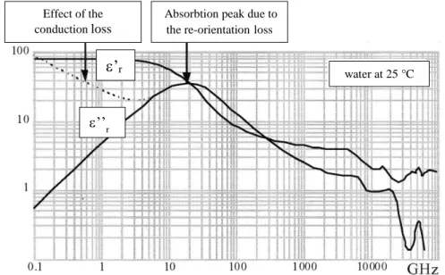
' ''     tg (39)

Figure 1.3 shows that water is transparent to microwaves at low

frequencies because of the low values of ’’. If salts in solution are

present, the phenomenon of conduction losses takes place at frequencies under 1 GHz. The energy dissipation is high in the microwave band, and is due to the mechanism of re-orientation loss, which is maximum at the frequency of 18 GHz. Nevertheless, the latter isn’t the operating frequency of the microwaves ovens, which operate at 2.45 GHz, as has been previously pointed out. The reason is related to the penetration depth

(p), defined as the depth at which the power drops to 1/e of its value at

surface: 2 1 ' ' ' 1 ' 1 2                  _P (40)

A very high value of ’’ causes a very little penetration depth: the wave is

strongly attenuated and heating is localized near the surface. If ’’ is very

low, the penetration depth is very large: the wave is slightly attenuated and the material is almost transparent to EM radiations. In the latter case the generated power density is negligible.

Therefore, at the frequency of 2.45 GHz there is a compromise between an acceptable penetration depth and an efficient heating process.

Food materials are in general not good electric insulator nor good electric conductors, thus fall into the category of lossy dielectric materials. Both

(26)

relative dielectric constants and loss factors of foods are largely influenced by moisture and salt contents, as well as by structure. For instance, the relative dielectric constant of cooked ham for 2450 MHz (72) at room temperature is very close to the value of distilled water, while the relative dielectric loss factor is twice that of free water (23 vs. 10.3). At 2450 MHz, Red Delicious apples with 87.5% moisture content have a relative dielectric loss factor of 11.2, slightly larger than that of free water. Upon removal of moisture content in drying, both relative dielectric constant and loss factors of Red Delicious apples sharply decrease [60].

Figure 1.3 Dielectric permittivity of water

Effect of the conductionloss

Absorbtion peak due to the re-orientationloss

’r ’’_r

(27)

CHAPTER 2 Batch tests: apples microwave drying

With the aim of analysing microwave drying processes, a new microwave drying system was developed which can automatically and continuously adjust the power levels by acting on the magnetron duty cycle time in order to control the product temperature. The signal for realizing feedback temperature control was obtained looking inside the illuminated MW chamber by an IR temperature equipment; the latter allowed to detect the instantaneous maximum temperature among the sample slices distributed randomly on the turning table. For the first time the feedback signal was no more related to a single arbitrarily chosen slice inside the MW chamber, which can affect results [33], but to the actual hottest one. Air temperature, humidity and speed were also controlled while the sample-holding turntable was suspended to a technical balance located on the top of the oven for online mass measurement [51]. Considering that microwave drying kinetics mainly depend on moisture diffusion phenomena since external and internal heating resistances become irrelevant to heat transfer mechanism, the ability of realizing experimental drying texts featured by constant temperature levels suggested to process the weight loss data by using a 2D unsteady analytical model for mass diffusion inside isothermal samples. Thus, the effective mass diffusivity [33-35] was determined and, as a consequence, the drying process prediction was allowed [87].

2.1 Experimental set-up

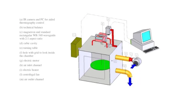
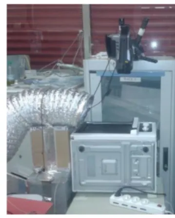
Drying was performed in a pilot plant, Figure 2.1, projected for general purposes in order to encompass different loads, i.e. different materials and samples distributions, weight, size. Hence, it has been aimed that the illuminated cavity could behave as a reverberating chamber, at least in the central space, due to the superposition of multiple modes. A large (with respect to volume where the samples under test were placed) cavity was then required, thus generated microwaves illuminate an insulated metallic

cubic chamber (1 m3). The microwave pilot plant was equipped with a

(28)

stirrer rotating at 250 rpm was employed to enhance the microwave power distribution inside the cavity.

A teflon rotating tray (50 cm diameter, 22 rpm) housed the samples under test and was connected to a technical balance (Gibertini EU-C 1200 RS) located on the top of the oven. The balance allowed real-time mass measurements. The tray was rotated at 10 rpm on a ball bearing shaft driven by an electrical motor.

An external centrifugal fan facilitated the moisture removal by forcing external air into the cavity; the renewal air flow was kept constant throughout the experiments by controlling the inverter feeding the fan electric motor. The channel feeding the external air flow was equipped with an electric heater controlled by a thermocouple placed on the air expulsion channel. The relative humidities and temperatures both of the exhaust and external air were measured by hygrocapacitative sensors (BABUC/M, LSI LASTEM Srl). A suitable combination of electric heater power and renewal airflow was selected in order to realize a fixed temperature level inside the illuminated chamber, with a reduced gap (about 10°C) between inlet and ambient air temperatures.

An IR equipment (thermaCAM flir P65) looked inside the oven through a hole 70 mm diameter properly shielded with a metallic grid trespassed by infrared radiation arising from the detected scene but impermeable to high-length EM radiation produced by the magnetron. The camera was

Figure 2.1 Microwave pilot plant heating system

(a) IR camera and PC for aided thermography control (b) technical balance (c) magnetron and standard rectangular WR-340 waveguide with 2:1 aspect ratio (d) cubic cavity (e) turning table

(f) hole with grid to look inside the chamber

(g) electric motor (h) air inlet channel (i) electric heater (l) centrifugal fan (m) air outlet channel

(29)

Batch tests: apples microwave drying 19 calibrated to account the presence of grid as follows: the temperatures of a large apple slice, cooled from 90 °C to 35 °C, were simultaneously recorded by the IR equipment and by a thermocouple placed on the surface of the target. The emissivity of the target was set to 1, while the air temperatures inside and outside the cavity were set to the same levels adopted during the experiments; thus the reflected ambient temperature was fixed and IR thermography readout was allowed. A second order polynomial related the two measured temperatures.

The measured data, i.e. samples weight, internal and external air temperature, the reflected magnetron energy and duty cycle, were transferred to a personal computer each minute for control and recording purposes. Power control based on thermography temperature readout was accomplished governing an I/O board (AT MIO 16XE50, National Instruments, TX, USA) with a suitably developed Lab View 7.1 code (National Instruments, TX, USA). In particular, the instantaneous maximum temperature in the detected scene was communicated via RS232 to the controlling code each 0.7 seconds.

2.2 Experimental procedure

Preliminary experimental tests were carried on white apples (Golden delicious); their initial moisture content was 86% wet base. Apples were handy peeled, shaped as cylindrical pieces with a diameter of 20 mm, 10

mm height, and finally distributed on the tray. The total amount of samples considered for each trial was 300 g. Weight changes during MW drying were registered on line by the technical balance.

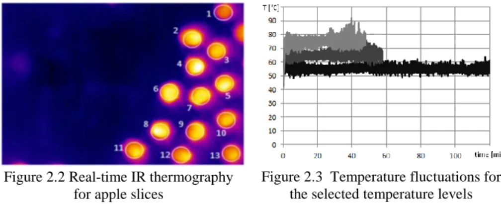
Figure 2.2 Real-time IR thermography for apple slices

Figure 2.3 Temperature fluctuations for the selected temperature levels

(30)

The IR system acquired the instantaneous surface temperature map inside the illuminated cavity gathering in the IR scene a number of samples covering about 20% of total weight (see Figure 2.2). The code scanned for the maximum temperature among the samples appearing in the IR image under test. Because of the turntable rotation, different samples were individuated by analysing different images. Then code automatically adjusted the magnetron delivered power by operating it in intermittent mode with constant power density; an on-off control was then set inside a specified differential band (±1°C) over the target temperature. The code also deliberated the end of the experimental test when the actual moisture content achieved a conventional fixed value of 20%.

Three selected temperature levels were chosen for processing the samples under test, namely 55, 65 and 75 °C; for all of them the internal air temperature was set to 30°C with an air speed equal to 2.5 m/s on the tray layer. The external relative humidity was controlled by an air

conditioning system so to realize 6 gw/kga. The renewal air flow was fixed

to 25 m3/h in order to contain the inlet temperature excess within few

degrees. All the experiments were repeated in triplicates and average values were processed.

2.3 Experimental results

2.3.1 Temperature control during MW heating

The capability of the MW system to keep the controlled temperature during MW drying at the desired values, namely 55, 65 and 75 °C, is shown in Figure 2.3. The average of maximum temperatures recorded on apples’ surface was close to the corresponding setpoint values within a difference value of 0.2 °C (Table 2.1). Temperature ﬂuctuations became larger while the process goes on, because of the increase of the power density in the last phase of the drying period due to the mass samples’ reduction. In order to quantitatively show the addressed trend, the drying period was divided into two similar parts and the temperatures standard deviations were calculated for these two periods (Table 2.1). The maximum temperature overshoot recorded during the last period of drying at 75 °C was 17.1 °C, thus showing that a product charring could take place and that temperature control became critical at high temperatures and for long time heating. This problem could be overcome by

(31)

Batch tests: apples microwave drying 21 introducing in MW oven a ‘‘mechanical moving mode stirrer’’ to assure more uniform EM-ﬁeld distribution.

T [°C] Tavg [°C] Tmax-Tavg [°C] Tmin-Tavg [°C] S.D. S.D. (I half) S.D. (II half)

55 55.2 8.9 6.9 1.9 1.9 1.8

65 65.2 11.1 7.6 2.8 2.3 3.2

75 75.1 17.1 9.5 3.1 2.7 3.3

Table 2.1 Set temperatures, averages, temperature oscillations and standard deviations (SD) during ﬁrst and second half of drying time by microwave of apple slices.

The Figure 2.3 showed that higher the temperature was, higher the temperature oscillations became. This outcome was evidenced evaluating the standard deviations with respect to the corresponding target values, where increasing values were reported for increasing temperatures. Such behaviour could be a consequence of the reduction in dielectric loss factor with temperature increase which requires higher time to keep surface temperature ﬁxed. As a consequence, the instantaneous overall temperature level of the slices increased. The temperature oscillations were not symmetrical if compared to the average temperatures, in

particular minimum temperatures (Tmin) were closer to the corresponding

average values than maximum temperatures, (Tmax). In fact, setting-on the

magnetron, the temperature increases took place faster than temperature decreases due to the slower radiative-convective cooling.

2.3.2 Drying curves

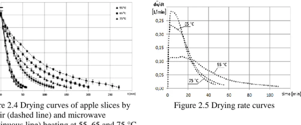
Assuming that the measured weight loss was equally distributed for all the samples, it was possible to evaluate the drying curves for the three selected temperature levels. Apple drying curves by hot air and MW, at 55, 65 and 75 °C are shown in Figure 2.4. As expected, apples drying were faster at higher temperatures, with a reduction of drying time that for hot drying was proportional to the increasing of temperature.

MW heating reduced signiﬁcantly the drying time if compared to convective one. MW absorption provokes internal water heating and evaporation, greatly increasing the internal pressure and concentration gradients and thus the effective water diffusion [18].

Moreover, as reported elsewhere [19], high temperature achieved during the heating cause the solubility of pectic material (apples are rich in

(32)

pectins) causing a lowering of rigidity of the cellular tissue, therefore a lower resistance to water transport.

The effect of a temperature increase from 55 to 65 °C reduced to about one half the MW drying time, while the increase from 65 to 75 °C reduced the drying time of only 20%. Probably the higher levels over the temperature set at 75 °C were able to produce a higher pectin gelation phenomena, thus changes in the apple microstructure that delayed the release of water from the matrix to the exterior because of the decrease in porosity or intra-cellular spaces.

Lastly, the slower drying in hot air can be explained recalling that in the convective drying samples temperatures were lower than the air temperature. The gap between air and sample temperatures was always decreasing as the drying process goes on because in the early stages sensible heating dominates, while later the progressive reduction of the evaporation rates was responsible for lower cooling rates. At their best, samples temperatures aimed to the set point values at the very end of the drying process (data not reported). On the opposite, thermal transients featuring MW processing lasted no more than one minute and were hardly appreciable in Figure 2.3.

Apples during MW processing showed typical drying rate, obtained taking the time-derivative of the corresponding curves represented in Figure 2.4. Their behaviour showed the typical trend for fruit drying: after an initial thermal transient, warming up period, when increasing moisture

gwater

gdry matter

Figure 2.4 Drying curves of apple slices by hot air (dashed line) and microwave

(continuous line) heating at 55, 65 and 75 °C.

Figure 2.5 Drying rate curves

removal rates were realized, the rate of moisture removal was constant for a short period and then fell off continuously [20].In warming up period,

(33)

Batch tests: apples microwave drying 23 microwaves heated without intermittence until the set point temperature was attained. The high content of water (85%) in apples was the main responsible for an efﬁcient internal heat generation causing

an increase in product temperature which in turn produced higher diffusion rate. In particular the drying rate curves (Figure 2.5) exhibited a linear (almost adiabatic) increase in evaporated mass; all the curves were ﬁrst overlapped and then increasing temperatures were responsible for slightly decreasing slopes due to the decrease of the dielectric loss factor and, in turn, to reduced MW absorption. Then, when the internal resistance to transport liquid water to the surface increased, thereby lowering the drying rate, the falling rate period occurred. Hence, internal diffusion may be assumed to be the mechanism responsible for water loss during the drying process. In the last phase of the falling period, since free water content was vanishing, the absorbed MW energy was mainly used to balance convective heat losses from the sample [21]. The thermal conductivity attained its minimum, while at the same time, as a consequence of the mass sample reduction, power densities increased. These occurrences, considering that only surface temperature was controlled, caused the establishment of a temperature gradient inside the sample where the core temperature was greater; thus, the related positive pressure generated inside forced out faster the lasting moisture. While the process further goes on, the addressed phenomena was enhanced considering that higher volumetric heat generation rates were realized.

2.4 The analytical model

Several models have been proposed to describe the rate of water loss during drying processes [22-29]. Among them, the description in terms of the effective diffusivity appears to be more adequate than the ones steaming from empirical kinetics: in facts, the latter don’t exhibit a general validity being related to specific load and boundary conditions features [39].

The mass transfer takes places according to the Fick’s first law (similar to Fourier law), which relates the diffusive flux to the concentration under the assumption of steady state. It postulates that the flux goes from regions of high concentration to regions of low concentration, with a magnitude that is proportional to the concentration gradient (spatial derivative), or in simplistic terms the concept that a solute will move from

(34)

a region of high concentration to a region of low concentration across a concentration gradient. In two or more dimensions, the law is:

     D J (1) where:

- J [kg/(m2∙s)] is the "diffusion flux" and measures the amount of

substance that will flow through a small area during a small time interval.

- D [m2/s] is the diffusion coefficient or diffusivity

- Ω [kg/m3] is the concentration

Considering eq. (1) and the mass conservation in absence of any chemical reactions, Fick’s second law can be derived, thus obtaining an equation analogous to the fundamental equation of conduction heat transfer:

       2 D t (2)

Usually, when weight loss of dried products is described, the water mass fraction (x) on dry basis is used; the latter parameter is defined as follows:

x = mw/ms= mw/(s∙V) = (mw/V)∙(1/s) = Ω/s (3)

where:

mw is the mass of the water; ms ands are the mass and the density of the

dry matter, respectively; V is the volume of the sample. Thus, using eq. (3), eq. (2) becomes:

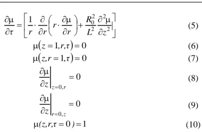
x D t x _ __₂   (4) With the aim of determining the effective diffusivity, the decrease of water in the apple slices has been described through an analytical model based on the local mass balance expressed by eq. (4), assuming isothermal conditions, constant properties, negligible shrinking and cylindrical shapes for samples, Figure 2.6. Considering first type boundary conditions, the dimensionless equations turn out to be:

(35)

Batch tests: apples microwave drying 25                            2 2 2 2 0 1 z L R r r r r τ (5)



1



0  z ,r,τ (6)



1



0  z,r ,τ (7) 0 0      ,r z z (8) 0 , 0      z r z (9) 1 0   (z,r,τ ) (10)

where: (z,r,) = (x(z,r,)-xe)/(x0-xe) is the normalized moisture ratio, x

being the mass fraction of the water on dry basis; xe and x0 are the

unperturbed air and the initial mass fractions of the water in the apple

slices; z = Z/L and r = R/R0 are the dimensionless axial and radial

coordinates, 2∙L and R0 being the height and the radius of the cylinder,

respectively;  = t/t0 is the dimensionless time, with t0 = R02/D.

Figure 2.6 Sample geometry

The problem being linear and homogeneous, the solution of the problem may be written as the product of two partial solutions, each one

depending on a single spatial coordinate, (z,r,) = (z,)2(r,). The

(36)





1 0) , ( 0 0 , 1 L R 1 0, 1 1 2 1 2 2 2 0 1                       z z z z z





1 0) , ( 0 0 1, r r r 1 2 0, r 2 2 2 2                                 r r r r

Both the two sub-problems are well-known, the former being related to the infinite slab, the latter to the infinite cylinder; they were solved by the separation of variables method yielding:

 

  

 





 







  2 n 1 n n n 1 z, c G z Exp λ (11)

 

  

 





 







  2 n 1 n n n 2 r, d F r Exp (12)

where Gn(z) = Cos[λn (L/R0)z] and Fn(r) = BesselJ0(n∙r) are the eigen

functions and λn, n are the related eigenvalues arising from the

characteristics equations: Cos[λn (L/R0)] = 0, BesselJ0(n) = 0.

2.5 Data reduction

Data reduction was carried-on by processing the falling rate period, when the resistance to species transfer by diffusion in the product is much larger than the resistance to species transfer by convection at the surface. Such an occurrence can be shown evaluating the mass transfer Biot

number, Bi = (hm L0)/D, where hm is the mass transfer coefficient, L0 is

the reference spatial coordinate. In the case of the air, the mass transfer

coefficient can be estimated as hm =h/(ρ∙c), 1/h being the thermal

resistance to heat transfer, ρ and c being the mass density and the specific heat of the air [31]. The magnitudo orders of the reference length and of

the mass diffusivity are 10-2 and 10-9, respectively, thus the Biot number

turns out to be much larger than unity. Accordingly, first type conditions on the wall are properly involved in equations (6) and (7) [32].

On the other hand, the use of the above model including the spatial dependence rather than a concentrated parameters model, was suggested by considering that the time extend needed for the apple moisture content

(37)

Batch tests: apples microwave drying 27 to decrease from 86 to 20% is small when compared to the sample

characteristics time, R02/D.

When performing measurements, it was assumed that the average weight loss for samples under test was described by the above model. Due to the complexity of the response model, the Levenberg Marquadt technique based fitting method has been selected. The technique enables to process non-linear models with an arbitrary number of parameters. Thus, the optimal choice for matching experimental and theoretical data was accomplished by minimizing the RMSE merit function:

 





1 2 1 2 1 N / i i i,D t N RMSE           



 (13)

where (i, ti) are the N experimental normalized moisture content taken at

the corresponding times ti, the function - is the functional relationship

given by the model for the average normalized moisture ratio, D being the unknown diffusivity.

The number of terms in the sum needed to evaluate - was chosen when

the corresponding RMSE variation, Δ, was less than 0.001.

Figure 2.7 Analytical prediction (continuous lines) vs experimental trend (falling rate period)

(38)

2.6 Results and discussion

Experimental curves and the corresponding analytical ones resulting from data reduction are reported in Figure 2.7 for the three temperature level at hand. The maximum standard deviation of the experimental data was

equal to 0.28 gwater/gdry matter.

A satisfying agreement between experimental and analytical data exists and is confirmed by the corresponding correlation coefficients, as shown in Table 2.2. In the same Table, the resulting diffusivities are reported; as expected, the effective mass diffusivity increases with temperature increasing while quantitative results seem to be consistent with the ones reported in literature. In particular, the values of apple effective

diffusivities reported by some authors ranges from 1.1∙10-9 to 6.4∙10-9

depending on airflow and air temperature conditions [35-38]; however, the results presented in this work should be more appropriate since the analytical model holds strictly for isothermal conditions. Such occurrence is closely realized by the present experimental set-up rather than by traditional hot-air heating or by microwave heating without temperature control. In the Table 2.2 are also reported the number of terms needed in the sum and the corresponding RMSE variation.

T [°C] D [m/s2_] _Terms _{RMSE [g}

w/gdm] Δ 104 Correlation Coeff.

55 °C 2.50210-9 ₁₀ _0.10932 _6.426 _0.992

65 °C 5.60110-9 ₁₆ _0.07945 _8.821 _0.995

75 °C 6.40110-9 ₁₂ _0.14421 _8.306 _0.991

(39)

CHAPTER 3 Batch tests on water and oil

Food processing is one of the most successful and largest application of microwaves (MW) since the presence of moisture in the food, which can couple with microwaves easily, facilitates heating thus allowing to realize shorter processing times. On the other hand, the uneven temperature distribution inside the products processed is one of the major obstacle to the diffusion of this technique. This problem can be reduced by acting both on the illuminating system and on target food.

In this chapter, after a brief description of the numerical method on which the software in use is based, the latter is validated through the comparison with the solutions obtained with another software for a simple case. Then, the problem at hand is presented. In particular, thermal response for water and oil samples, placed in a special thermoformed tray, with different size and orientation has been studied. The first aim was to show that temperature predictions can recover experimental results.

Afterwards, uniformity in temperature distribution was investigated by both performing numerical runs and corresponding experimental tests in a pilot plant. With reference to the former approach, samples under test were assumed to be homogeneous dielectric liquid/solid media in which an electromagnetic wave propagates originating dissipative phenomena accounting for energy generation. As a first attempt, natural convection into the samples is neglected in order to test the ability of the mathematical model presented in this study to correctly explain the phenomena of microwave heating within the target. This hypothesis comes true if time measured in the appropriate scale is small. As a further consequence of such hypothesis, cooling by convective/radiative transfer with surroundings is neglected too [86].

3.1. The finite element method

The finite element method (FEM) [62] is a numerical procedure which allows the transformation of analytical equations (for the case at hand, energy balance equations, Maxwell equations and the related boundary conditions) into algebraic equations. The aim is the research of

(40)

approximate solutions when there aren’t mathematical instruments able to solve the analytical equations exactly. In the specific case, a FEM software, COMSOL Multyphisics [61], has been used; it allows to define, in the pre-processing phase, the physical field of the problem. Then, the geometry is built using the same software or, if available, it is externally built by a CAD software and is imported, imposing the boundary conditions and the constraints. Afterwards, the type of element is chosen and the mesh is generated. The latter depends on the problem at hand. In particular, the elements can be:

- Monodimensionals: problems with a single dependent variable.

- Bidimensionals (triangles or squares) : problems with two

dependent variables

- Tridimensionals: (tetrahedra, prisms, hexahedral): problems with

three dependent variables

Finally, during the solver phase, the software finds the numerical solution. A number of solvers are available according to the type of problem, stationary or time dependent.

The goodness of the approximated solution has to be checked; in particular, the convergence of the solution depends especially on the shape function and the elements size. So the error drops approaching the nodes, that is reducing the size of the elements; it’s necessary to find a compromise between the computational time and the level of discretization: the latter could be increased where needed and elements with a proper shape, compliant with geometry, could be used.

3.2. Comsol vs Ansys HFSS: the software validation

With the aim of validating the software before its use, a simple problem was solved with another FEM software, Ansys HFSS, and the solution was compared with the one obtained by Comsol Multyphisics. As reference, the geometry studied in [63] was assumed. The problem at hand involved a single mode cylindrical microwave cavity, crossed by a

(41)

Batch tests on water and oil 31 cylinder of still water, whose axis was overlapped to the one of the cavity. The radius of the cavity, the height and the radius of the material load are 63.5 mm,150 mm and 50 mm, respectively. A magnetron, whose power was set to 1 W, produced microwaves supplied by a rectangular waveguide (WR340), emitting at a frequency of 2.45 GHz. Water dielectric properties were assumed to be independent of temperature; in particular, the real and the imaginary parts of the dielectric permittivity were set to 78 and 9.8, respectively. The geometry was generated in Solidworks ® and was imported in Comsol and in Ansys HFSS (Figure 3.1). For both software, the sampling densities of 6 mm for the water and 17 mm for the air were assumed.

0 20 40 60 80 100 120 140 160 180 200 0 25 50 75 100 125 150 A b s(E z) [V/ m ] x [mm] Comsol Hfss

Figure 3.2 Modulus of the “z-component” of the electric field

0 10 20 30 40 50 60 70 80 0 20 40 60 80 100 120 140 160 A b s(E x) [V/ m ] x [mm] Comsol Hfss

Figure 3.3 Modulus of the “x-component” of the electric field

Figure 3.1 Scheme of the single mode cavity

y _x

(42)

Figs. 3.2 and 3.3 show the comparison between the component of the electric field along the “z axis” and “x-axis”, while the third component is negligible.

The maximum relative difference between the areas underlay by the curves is equal to 7.4 % for the z-component and to 7.8 % for the x-component. It was verified that, increasing the number of elements, the curves became closer and closer.

Finally, Figure 3.4 shows a bi-dimensional map of the electric field norm generated by Comsol. It’s easy to recognize the wave propagation along the waveguide and the different field patterns inside the water and the air.

3.3. Batch tests: the problem at hand

The microwave system used to perform the experiments is schematically represented in Figure 3.5 and its geometry was generated in Solidworks ® and was employed for numerical simulations.

In particular, Figure 3.5 is the scheme of a domestic microwave oven (Whirpool MWD302/WH), whose cavity size turns out to be 290x203x285 mm. Samples under test (SUT) are heated by microwaves produced by a magnetron with a nominal power of 900 W and emitting at a frequency of 2.45 GHz. A rectangular (76.5x40.0 mm) waveguide, sealed at one end, is used as a collimator and connects the magnetron to the cavity. Inside the collimator, on the upper side of the waveguide, near the radiating aperture, it is visible a little semisphere which acts to shield the magnetron from back-illumination. The waveguide port opening on