Alma Mater Studiorum
Universit`
a degli studi di Bologna
Scuola di Dottorato in Scienze Matematiche, Fisiche ed Astronomiche
DOTTORATO DI RICERCA IN ASTRONOMIA
CICLO XXVI
The evolution of massive clumps
in star forming regions
Dottorando: Supervisore:
Andrea Giannetti Dr. Jan Brand
Relatore: Coordinatore:
Chiar.ma Prof.ssa Loretta Gregorini Chiar.mo Prof. Lauro Moscardini
Settore Concorsuale: 02/C1 - Astronomia, Astrofisica, Fisica della Terra e dei Pianeti Settore Scientifico-Disciplinare: FIS/05 - Astronomia e Astrofisica
Questa tesi `e stata svolta nell’ambito delle attivit`a di ricerca dell’Istituto di Radioastronomia
(Istituto Nazionale di Astrofisica, Bologna)
The research presented in this thesis was carried out as part of the scientific activities of the Istituto di Radioastronomia (INAF, Bologna)
Contents
1 Introduction 9 1.1 Interstellar Medium . . . 10 1.2 Molecular clouds . . . 11 1.2.1 Dust . . . 13 1.3 Star formation . . . 141.3.1 Low-mass star formation . . . 15
1.3.1.1 Mass-Luminosity diagram . . . 18
1.3.1.2 Depletion and deuteration in low-mass starless cores . . . 20
1.3.2 High-mass star formation . . . 22
1.3.2.1 Evolutionary phases of high-mass stars . . . 24
1.4 The influence of high-mass stars on their environment . . . 27
1.5 Outline of the thesis . . . 29
2 The Bayesian approach to statistics 31 2.1 The Frequentist approach . . . 32
2.2 The Bayesian approach . . . 33
2.2.1 The rules of probability and the Bayes theorem . . . 35
2.2.2 Marginalisation . . . 43
2.2.3 Model comparison and Ockham’s razor . . . 45
2.2.4 The advantages of the Bayesian approach . . . 47
3 Physical properties of massive clumps 49 3.1 Chapter summary . . . 49
3.2 Introduction . . . 51
3.3 Sample and tracer . . . 54
3.4 Observations and data reduction . . . 55
3.5 Results and analysis . . . 56 5
CONTENTS 6
3.5.1 Ammonia line profiles and properties . . . 56
3.5.2 Temperatures from ammonia . . . 58
3.5.3 Ammonia abundances . . . 60
3.5.4 Clump masses, diameters and gas densities . . . 61
3.5.5 Spectral energy distribution . . . 64
3.5.6 Stability and dynamics of the clumps . . . 69
3.5.6.1 Velocity gradients . . . 70
3.5.7 Water maser emission . . . 72
3.6 Discussion . . . 72
3.6.1 The mass-luminosity diagram . . . 76
3.6.2 Properties of sources in different stages of evolution . . . 82
3.6.2.1 Temperatures . . . 82
3.6.2.2 Sizes . . . 83
3.6.2.3 Densities . . . 84
3.6.2.4 Mass . . . 88
3.6.2.5 Velocity and linewidth . . . 88
3.6.2.6 Virial parameter . . . 89
3.6.2.7 CO depletion . . . 92
3.6.2.8 Chemical tracers of Hot Cores and star formation 94 3.7 Observational classification of high-mass clumps . . . 100
3.8 Summary and conclusions . . . 100
4 CO depletion and isotopic ratios 105 4.1 Chapter summary . . . 105 4.2 Introduction . . . 107 4.3 The Sample . . . 109 4.4 Observations . . . 110 4.5 Results . . . 110 4.5.1 Distance . . . 110 4.5.2 Excitation Temperatures . . . 111
4.5.3 Isotopic Abundance Variations in the Galaxy . . . 112
4.5.4 Optical Depths and Column Densities . . . 115
4.5.5 Column density of molecular hydrogen . . . 118
4.5.6 Masses . . . 119
4.6 Discussion . . . 120
4.6.1 Linewidths and Temperatures . . . 120
4.6.2 Refined Estimate of the Isotopic Ratios . . . 123
CONTENTS 7
4.6.3.1 RATRAN Modelling . . . 131
4.6.3.2 RATRAN Modelling of Individual Sources . . . 135
4.6.4 Stability of the Clumps . . . 139
4.7 Summary and Conclusions . . . 142
5 Later stages of massive star formation: the NGC 6357 complex 151 5.1 Chapter summary . . . 151
5.2 Influence of massive stars on nearby molecular gas . . . 153
5.2.1 Introduction . . . 153
5.2.2 Observations and data reduction . . . 156
5.2.3 Results and discussion . . . 158
5.2.3.1 Morphology . . . 158
5.2.3.2 Temperatures . . . 160
5.2.3.3 Column densities . . . 163
5.2.3.4 Opacities and visual extinctions . . . 164
5.2.3.5 Dust . . . 165
5.2.3.6 Molecular abundances . . . 168
5.2.3.7 LTE masses and volume densities . . . 169
5.2.3.8 Non-LTE analysis . . . 170
5.2.3.9 Virial masses . . . 176
5.2.3.10 Selective photodissociation . . . 176
5.2.3.11 Ionisation front and geometry of the region . . . 178
5.2.3.12 Comparison with massive clumps in early stages of evolution . . . 179
5.2.3.13 Pismis 24 13 (N36) . . . 181
5.2.4 Summary and Conclusions . . . 181
5.3 Past and current star formation in NGC6357 . . . 185
5.3.1 IR photometry . . . 186
5.3.2 Large scale distribution of IRAC sources . . . 188
5.3.3 Stellar population of Pismis 24 . . . 189
5.3.4 The K luminosity function and the initial mass function of Pismis 24 . . . 193
5.3.5 Age and initial mass function of Pismis 24 . . . 194
5.3.6 Star formation in Pismis 24 and in G353.2+0.9 . . . 198
5.3.7 Summary . . . 198
CONTENTS 8
A Rules of probability 221
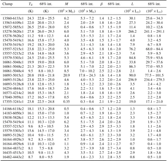
B Appendices to Chapter 3 225
B.1 Comments on individual sources . . . 225
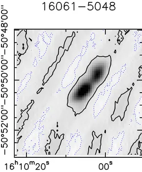
B.1.1 16061−5048c4 and 16435−4515c3 . . . 225
B.1.2 17355−3241c1 . . . 226
B.1.3 Undetected sources . . . 226
B.2 SED fits . . . 227
B.3 Tables and figures . . . 229
C Appendices to Chapter 4 249 C.1 Tables . . . 249
C.2 Spectra . . . 268
Chapter 1
Introduction
Human beings have always had the instinct of looking up at the sky. The stars there are the fundamental building blocks that make the visible Universe the way we see it, and they are born and die over timescales much longer than the human life span; thus the celestial sphere may appear to the eye as static and immutable for thousands of years. However, though stars were certainly formed in large numbers in the past, star formation is occurring even now in our own Galaxy. To understand that star formation is a process active even today took a long time, and this idea did not come up until the middle of the last century (Ambartsumian 1947, 1949), because stars are born in the densest parts of molecular clouds, and the whole process is hidden from view by the very same gas and dust out of which they are formed. To penetrate this obscuring curtain we must use longer wavelengths than our eye is able to perceive.
The effort to unveil what happens behind this curtain is well motivated: not only do stars determine how galaxies appear to us, but they are also crucial for life. On the one hand, within them almost all the elements heavier than helium are formed and then released into the interstellar medium in the final phases of their lives; on the other hand, complex organic molecules are commonly observed in sites of active star formation. Among the complex species detected in interstellar space there is the simplest sugar, glycolaldehyde (e.g., Hollis et al. 2000; Beltr´an et al. 2009), a precursor of ribose, which forms part of the backbone of RNA. Last but not least, star formation is connected to the formation of planetary systems like the Solar system (e.g., Williams & Cieza 2011, for a review on proto-planetary disks). Thus, in the end, understanding the process of star formation has deep implications for understanding the formation of the Earth, how life developed here and ultimately whether the conditions of the Solar system are unique, or quite
1.1. Interstellar Medium 10
common in the Universe.
1.1
Interstellar Medium
Stars. Planets. These are the first things that come in mind when one thinks of our Galaxy. However, they occupy only a minor fraction of space in the Milky Way; the rest, the large volume between stars, is filled with diffuse gas, dust and radiation, generally referred to as the Interstellar Medium (ISM). The first indication of its existence was the presence of dark patches devoid of stars compared to nearby areas, in the photographic atlas of the Milky Way (Barnard et al. 1927). Since then, the ISM has been observed both in absorption and emission, in the continuum and in atomic and molecular lines.
The quantity and state of gas contained in a galaxy has relevant effects on its appearance, especially through star formation. The quantity of gas as a fraction of baryonic mass varies strongly between different types of galaxies and also amongst galaxies of the same type. Typical values range from ∼ 1% for elliptical galaxies, to ∼ 10% for spirals and even more for irregular galaxies. The ISM is mainly composed of hydrogen, while helium and metals (in the “astronomical” sense, i.e. all elements heavier than helium) represent respectively ∼ 10% and ∼ 1% (in number) of the atoms. Despite their low abundance, metals are crucial for the physical and chemical evolution of the interstellar matter (through heating & cooling).
The ISM is characterised by a wide range of temperatures and densities, and it can be both ionised and neutral. Because of this, the ISM is usually divided in three different states or phases: hot, warm and cold, according to its temperature. The typical temperature of each phase is such that they are in approximate pressure equilibrium. However, regions that are not in pressure equilibrium clearly exist, such as Hii regions, that are overpressurised and expanding, or molecular clouds, that may be self-gravitating. The ISM phases are also classified according to their state of ionisation. Therefore, as a first approximation, the ISM can be separated
into: hot ionised medium, warm ionised/neutral medium and cold neutral medium.
The typical properties of these distinct phases are summarised in Table 1.1. This simple picture of discrete ISM phases is complicated by turbulence, con-tinuously mixing the interstellar matter, and, in some cases, thermal instability becomes a second order effect. The efficiency of turbulence in turning discrete phases into a continuum is still matter of debate (see, e.g., Audit & Hennebelle 2008; Vazquez-Semadeni 2009).
1.2. Molecular clouds 11
Table 1.1: Physical properties of ISM phases, from Draine (2010) and Hennebelle & Falgarone (2012).
Phase Temperature Density Filling factor
(K) (cm−3)
HIM > 3 × 10⁵ 4 × 10⁻³ ≈ 0.5
WIM & Hii regions 3 × 10³− 104 0.3 − 104 ≈ 0.1
WNM 500 − 8 × 10³ 0.3 − 0.6 ≈ 0.4
CNM(1) 100 30 ≈ 0.01
CNM(2) 10 − 50 103−6 ≈ 10−4
Notes.(1)Diffuse clouds;(2)Molecular clouds
1.2
Molecular clouds
The vast majority of the molecular gas (∼ 80% in the Milky Way) resides in giant cloud complexes. The filling factor of molecular gas is very low, i.e. the fraction of volume occupied by molecular clouds is very small compared to that occupied by atomic gas (see Table 1.1). However, these clouds are also the densest component of the interstellar medium, accounting for a significant fraction (∼ 13%) of the mass of the ISM (∼ 7 × 10⁹M
in the Milky Way; Draine 2010). The typical properties
of molecular clouds are shown in Table 1.2. The bulk of molecular gas is usually very cold, with temperatures around 10 − 20 K. Molecular rotational transitions may have very low energies above the fundamental state; CO, for example, has the lowest rotational transition only at 5.5 K above the ground state, and can thus be easily excited even in the very cold environments of molecular clouds, that therefore appear bright in some molecular lines. The line emission from molecules critically depends on the physical properties of the emitting medium, and one can use their emission to infer the conditions of the gas, such as its temperature and density.
The molecular gas is embedded in a more diffuse, atomic medium, which
partially shields the cloud from radiation, allowing the formation of molecules. In fact, molecules are always observed above a certain critical value of visual extinction AV (≈ 3 mag, Tielens & Hollenbach 1985). The linear sizes of the
atomic envelopes are typically several times larger than those of the embedded molecular complexes, with masses that can be comparable to those of the molecular gas (Blitz 1993).
a) Molecular Cloud
∼ 1 pc
∼ 0.1 pc
b) Molecular Clump
c) Molecular Core & Protostar
Figure 1.1: Clumpy structure of a molecular cloud. The panels show different
spatial scales: a) cloud, b) clump, and c) core and its embedded protostar. In a) and b) the linear scale is indicated in the bottom left or right corner.
1.2. Molecular clouds 13
Table 1.2: Physical properties of molecular clouds complexes and their components. The columns show typical values of the average particle number density, size, mass, linewidths and extinction in the optical, respectively. Adapted from Draine (2010).
Category ntot Size M Linewidth AV
(cm−3) (pc) (M
) (km s−1) (mag)
GMC complex 50 − 300 25 − 200 105− 106.8 4 − 17 3 − 10
Dark Cloud Complex 102− 103 4 − 25 103− 104.5 1.5 − 5 4 − 12
GMC 103− 104 2 − 20 103− 105.3 2 − 9 9 − 25
Dark Cloud 102− 104 0.3 − 6 5 − 500 0.4 − 2 3 − 15
Figure 1.1 illustrates that giant molecular clouds are highly structured entities (e.g., Blitz & Williams 1999), showing a hierarchical structure. Each cloud typically contains several dense and compact regions of size of the order of 1 pc, called molecular clumps. The space between the various clumps is filled with lower density gas. From observations we know that a fraction of this material is certainly molecular, while the remainder is atomic, with a higher temperature (20 − 40 K) with respect to the molecular component. The inter-clump gas represents only a minor fraction of the mass of the complex. Clumps are easily detectable at mm wavelengths through optically thin dust emission or molecular transitions. Moving to smaller spatial scales, clumps, like clouds, are not homogeneous. The smallest and densest regions in a clump are called cores. They have sizes of the order of 0.1 pc and they are often sites of active star formation, as revealed by the presence of embedded young stellar objects (YSOs) visible as point sources at infrared (IR) wavelengths.
1.2.1
Dust
Interstellar dust is the main source of extinction at long wavelengths, due to absorption or scattering of non-ionising photons; it dominates the Spectral Energy Distribution (SED) of the ISM for wavelengths longer than that of the Lyα line
(λ = 1215.67 Å), shortwards of which H ionisation occurs. In fact, the grains
absorb photons from the far-UV to the visible, and re-emit them at IR wavelengths.
The IR emission of diffuse interstellar matter shows two clear components,
reflecting a real difference in the grain size distribution. These two components have different temperatures: one is cold, with a temperature typically around 15 − 20 K,
1.3. Star formation 14
while the other is hot, with T ∼ 500−1000 K. The cold component is due to thermal emission from large grains (∼ 0.1 µm). These are in radiative equilibrium with the interstellar radiation field and self-radiate according to the Planck formula modified by the grain emissivity. The second component is generated, on the other hand, by very small grains (< 50 Å) and Polycyclic Aromatic Hydrocarbons (PAHs), that absorb a single far-UV photon, reaching temperatures of approximately 500 − 1000 K, and after which they rapidly re-radiate the energy at mid-IR and near-IR wavelengths.
Dust grains also play a very important role in the chemistry of the ISM. In fact, they offer a surface where atoms can accrete, encounter and react, redistributing the excess energy to the grain itself. This makes it possible for species like H2
to be formed much more easily in the interstellar space, because grains act as catalysts, thus making the reactions through which molecules are formed faster than those that happen in the gas phase. Furthermore, the dust competes with the gas to absorb far-UV photons. This is particularly relevant in molecular clouds, where dust shields the molecules from photons that can destroy them, in addition to the self-shielding effect (i.e. the molecules at the edge absorb the dissociating photons, protecting those deeper in the cloud) of some molecules such as H2or, to
a lesser degree, CO.
Dust also controls the abundances of metals in the gas phase, through accretion of these atoms onto the grains and destruction of the dust particles. A visible effect of these processes is, for example, the depletion of heavy elements in the interstellar medium, especially of those capable of forming refractory solids. The issue of grain composition has been widely debated and it is still not completely certain. It seems, however, that silicates and graphite or amorphous carbon are important components of interstellar dust.
1.3
Star formation
How molecular clouds are formed is still matter of debate; on the one hand they may be long-lived entities, supported against collapse by magnetic fields (e.g., Shu et al. 1987; Lada & Kylafis 1991) or, on the other hand, they can be transient structures, like atmospheric clouds (e.g., Glover & Mac Low 2007).
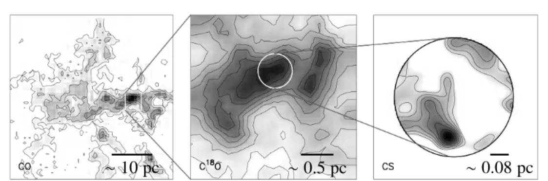
In Sect. 1.2 we saw how molecular clouds are not homogeneous entities, but present a significant substructure (cf. Fig. 1.1 and 1.2; a sketch and real data, respectively). Dense and filamentary structures are commonly observed within giant molecular clouds (e.g., Bally et al. 1987; Mizuno et al. 1995). These
1.3. Star formation 15
∼ 10 pc ∼ 0.5 pc ∼ 0.08 pc
Figure 1.2: Hierarchical structure of a cloud as observed in real data (Rosette cloud). The panels show a representative view of clouds, clumps and cores, respectively. Different tracers are used to make the different scales stand out: CO for the large-scale structure of an entire cloud, the optically thin C18O to isolate the column density peaks corresponding to clumps and the high density tracer CS to identify cores, the densest regions within the clumps. The Figure is taken from Blitz & Williams (1999).
structures in turn host clumps, out of which entire star clusters are formed, and cores, forming a single star or a small multiple stellar system.
For stars with a final mass above ≈ 8 M (see Sect. 1.3.2) the contraction
timescale of the protostar is shorter than the time needed to accrete all of its mass. This changes the evolution of the object with respect to its lower-mass counterparts, and therefore in the following we make a distinction between the formation of low-and high-mass stars.
1.3.1
Low-mass star formation
Solar-mass stars form following a (now) well-known sequence of evolutionary stages that can be easily observed in nearby molecular clouds. A classification of the evolutionary stages based on the SED slope at near-IR and mid-IR wavelengths was developed by Lada (1987), and shown in Fig. 1.3.
Figure 1.3 also shows a sketch of these phases, from a dense core within a molecular cloud to the “naked” star. The evolutionary phases can be summarised as follows:
1. Prestellar — Not all cores in a cloud are destined to collapse to form a star. Those that have the “right” initial conditions to permit collapse (i.e. they are
1.3. Star formation 16 d) c) b) a) ∼ 107yr ∼ 106yr ∼ 2 × 10⁵yr < 3 × 10⁴yr 0 yr Time
Figure 1.3: Spectral Energy Distributions (left) and sketch of the circumstellar environment (right), for Classes 0-III (see text for a description). Taken from Isella (2006).
or will become gravitationally unstable) are called prestellar cores. They are quiescent objects, made up of dense and cold material, typically embedded in an envelope of less dense gas. The cores are contracting, thus progressively increasing their density (this phase is not shown in Fig. 1.3).
2. Class 0 — A core with a sufficiently high density collapses under the action of gravity, marking the initial act of the star formation process. The regions with higher density become unstable first, and the collapse proceeds inside-out, progressively including material from more external regions in the cocoon, and accreting it onto the central object, increasing its mass. Any angular momentum from the original cocoon is conserved, increasing its
1.3. Star formation 17
rotation velocity as the radius shrinks, and giving rise to flattened structures. Molecular outflows perpendicular to the axis of rotation have been observed already in these stages (e.g., Saraceno et al. 1996; Bourke et al. 2005), implying that the outflow phenomenon appears very early in the process of star formation, and is directly linked to mass accretion. In fact, outflows
help to remove angular momentum, thus allowing/facilitating accretion.
Objects in such an early evolutionary stage are visible only at mm-/far-IR wavelengths (cf. panel (a) of Fig. 1.3).
3. Class I — The collapse of the core proceeds, making the density in the central parts increase so much that the material becomes opaque to its own infrared radiation. This causes the temperature to rise steadily, and the mate-rial is eventually dissociated and ionised. At this point the collapse has halted in the central regions, where a protostellar nucleus can be found, whose ma-terial is supported by thermal pressure. The mama-terial surrounding the embryo is now arranged in a circumstellar accretion disk, that continues accreting from the envelope. The protostellar nucleus is in turn accreting material from the disk; part of the angular momentum of the material is dissipated through a collimated bipolar outflow, allowing the gas to fall onto the protostar. The central object is still deeply embedded in a molecular and dusty envelope, and its emission is thus heavily extincted. From an observational point of view, disks, outflows and jets can be seen, e.g., through molecular line emission. During this stage, the protostar will become visible at near-IR wavelengths (cf. panel (b) of Fig. 1.3); it has a strong near-IR excess, mainly caused by the emission of the disk. This can be qualitatively reproduced modelling the disk as a superposition of black-bodies with different temperatures.
4. Class II — After ∼ few × 105yr most of the surrounding material has joined the circumstellar disk and the central object can be seen also in the optical. Mass accretion onto the protostar is still continuing. Classical T-Tauri stars are in this evolutionary stage. Class II objects still show signs of accretion and have a near-IR excess (cf. panel (c) of Fig. 1.3).
5. Class III — The material in the disk is slowly consumed (being accreted onto the central object or expelled by e.g. outflows) thus reducing the mass accretion. The central object does not show any near-IR excess any more (cf. panel (d) of Fig. 1.3). Due to the strong magnetic field of the protostars, they are much more luminous in X-rays than main sequence stars (e.g., Feigelson & Montmerle 1999) of the same mass.
1.3. Star formation 18
6. Main Sequence — After ∼ 107 yr H-burning is initiated: the star reaches
the zero age main sequence (ZAMS), the disk is completely evaporated and a planetary system may have formed from the disk. At this point, the radiation from the newly-formed star comes entirely from the stellar photosphere, and the star is visible in the optical.
1.3.1.1 Mass-Luminosity diagram
The evolutionary sequence identified in the low-mass regime (class 0-III, see Sect. 1.3.1) on the basis of the objects’ spectral slope in the IR was taken a step further by Saraceno et al. (1996). The authors collected and classified a sample of objects from class 0 to class II, and then constructed a diagnostic diagram comparing the mass of the circumstellar envelope and the total luminosity of the source.
Saraceno et al. (1996) show that classes 0 to II are found in different regions of the diagram (cf. Fig. 1.4, grey symbols and lines). For a given mass, less evolved objects have a lower luminosity. The evolution of a protostar in the low-mass regime is controlled mainly by its mass, that determines the total luminosity L, and by the quantity of circumstellar material M. M and L can be directly derived from the observations, and their combination provides a straightforward method to determine the evolutionary phase of a low-mass protostar. In the diagram, time increases in the vertical direction at first and then from right to left.
Molinari et al. (2008) extended this method to the high-mass regime (Fig. 1.4, black symbols and lines), finding that the mass-luminosity plot may also be used to infer the evolutionary stage of massive objects. In Fig. 1.4 black open circles show sources in the earliest evolutionary stage, and progressively more evolved objects are indicated by filled circles, asterisks and pluses. The evolutionary phase of the sources is inferred by their mm- and IR properties (see Chapter 3), and with the models described in Robitaille et al. (2006) and Robitaille et al. (2007). The curves represent the evolution of clumps with different initial envelope masses. Time evolves as in the low-mass case, increasing first in the vertical direction, and then from right to left (see also Sect. 3.6.1). The black solid line is the best fit to the sources likely hosting a ZAMS star. Whereas low mass-stars may form in isolation and can be relatively nearby, high-mass stars virtually always form in clusters (cf. Sect. 1.3.2) and since they are typically at larger distances due to their rarity, one cannot reach the same spatial resolution, and confusion with other sources in the cluster is an issue. Therefore, in this case, the luminosity and the mass are typically those of an entire high-mass star-forming region, rather than of
Figure 1.4: Mass-Luminosity diagram for low- (grey) and high-mass (black) regimes. Lines and symbols in grey are from Saraceno et al. (1996), for the low-mass regime. Class 0, I and II sources are represented respectively by open circles, filled circles and crosses, with the solid grey line representing the log-log linear fit to the Class I source distribution. The grey curves show the protostellar evolution in the low-mass regime, for different values of the final stellar mass. The black lines and symbols represent the sources in Molinari et al. (2008), for the high-mass regime; open circles show sources in the earliest evolutionary stage, and progressively more evolved objects are indicated by filled circles, asterisks and pluses. The curves represent the evolution of clumps with different initial envelope masses. The black solid line is the best fit for those clumps likely hosting a Zero Age MS star. The black dashed line is the log-log fit to the less-evolved massive sources. In both regimes, time increase in the vertical direction at first and then from right to left. Taken from Molinari et al. (2008).
1.3. Star formation 20
a single (proto)star.
1.3.1.2 Depletion and deuteration in low-mass starless cores
Low-mass starless cores have been studied extensively, with a high spatial resolu-tion thanks to their general nearness. These observaresolu-tions made it possible to derive the physical structure as a function of radius in the core; their column density-, volume density- and temperature at different radii are now well known, making it possible to study the chemical properties of the cores in detail.
At the low temperatures found in dense and quiescent regions of the clouds, the molecules can stick onto the dust grains, forming an ice coating (see e.g., Caselli 2011). One can calculate the rate at which molecules stick onto the grains, following the expression:
k= σv(T)ngS, (1.1)
where σ is the cross section of the grains, v(T ) is the mean value of the Maxwellian function describing the velocity distribution of the particles in a gas with tempera-ture T , ngis the volume density of the grains and S is the sticking probability. For
CO at 10 K, and assuming S = 1 in these conditions (meaning that each time a gas particle hits a grain it sticks to it), the adsorption (or freeze-out) timescale τadsis
(see Bergin & Tafalla 2007): τads = 1/k ≈
5 × 10⁹
n(H2)[cm−3]
yr, (1.2)
shorter than the free-fall timescale for n(H2)& 104 cm−3. Bacmann et al. (2002)
suggest that, from the comparison of CO and dust emission, the freeze-out becomes important for densities of molecular hydrogen above ∼ 3 × 104cm−3.
Dust emission traces well the H2, thus identifying the core and the location
where column density is maximal. Clear differences are found in the behaviour
of carbon- and sulphur-bearing molecules and nitrogen hydrides comparing the distribution of the emission of these different classes of molecules with that of the dust in the (sub-)mm regime. It is commonly found that the abundance of C-and S-bearing molecules tend to rapidly decrease towards the centre in low-mass starless cores (Caselli et al. 1999; Bergin et al. 2002; Tafalla et al. 2002; Zhang et al. 2009), where the density is higher and the temperature is lower, while nitrogen hydrides have constant- or much more slowly decreasing abundances. Figure 1.5
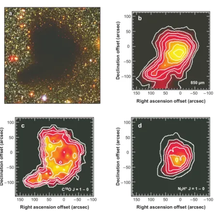
1.3. Star formation 21
Figure 1.5: Multiwavelength image of the molecular core B68, taken from Bergin & Tafalla (2007). The top left panel shows the obscuration region observed in the optical. The top right panel shows the dust continuum emission at 850 µm. The bottom panels show the integrated molecular emission of C18O(1 − 0) (left) and N2H+(1 − 0) (right). The different spatial distribution is clear, with N2H+(1 − 0)
closely following the emission profile of the dust, while C18O shows a ring-shaped
emission around the dust sub-mm emission peak.
ring-like, with a hole coincident with the peak of dust emission (and thus of the column density), on the other hand the emission of N2H+closely resembles that
of the dust. The different behaviour of these classes of molecules depends on the effects of the removal of CO from the gas phase, that triggers important changes in the chemistry of the core. An additional explanation may be that the atomic N, which has a low probability of sticking to grains (≈ 0.1, Flower et al. 2006) is only slowly converting into molecular nitrogen (Hily-Blant et al. 2010), which has similar sticking coefficient and binding energy as CO ( ¨Oberg et al. 2005; Bisschop
1.3. Star formation 22
et al. 2006). In particular, CO has a dominant role in the destruction of the N2H+
molecule (Bergin & Tafalla 2007, and references therein). Thus, the abundance of this molecule (and of ammonia, that is formed from N2H+; see e.g. Aikawa et al.
2005) increases where CO is depleted (e.g., Jørgensen et al. 2004). As long as N2does not reach abundances below those of N2H+and NH3, they can still form
and trace the dense gas where other molecules have a large degree of depletion, i.e. very reduced abundances. The same happens for deuterated molecules, which can become more abundant even by several orders of magnitude, with respect to normal conditions (e.g., Roueff et al. 2000; Loinard et al. 2001, 2002). As deuterium bonds are stronger than bonds with the most common hydrogen isotope, ion-molecule reactions are thought to be at the basis of these increased abundances (Millar et al. 1989). The presence of the ions at the beginning of the reactions is ensured by the
cosmic rays ionisation. The driving reaction for deuterium chemistry in the cold and dense environments of starless molecular cores is:
H+3 + HD ↔ H2D++ H2+ 230 K, (1.3)
which is slightly exothermic in the forward sense, favouring the formation of H2D+at 10 K, and increasing the deuteration of species involved in ion-molecule
chemistry. Moreover, considering also the following reactions
H2D++ HD ↔ D2H++ H2+ 180 K (1.4)
D2H++ HD ↔ D+3 + H2+ 230 K, (1.5)
one can reproduce the observed abundances of doubly or triply deuterated species (Roueff et al. 2000; Lis et al. 2002). Finally, because CO is the primary destroyer for H+3 and H2D+, the ratio between deuterated- and non-deuterated species may
increase even more (e.g., Caselli et al. 2002; Bacmann et al. 2003).
1.3.2
High-mass star formation
Whereas for low-mass stars the formation process is quite well-understood both theoretically and observationally, the analogous process in the high-mass regime is still far from being clear on both fronts, despite the attention dedicated to it in the last decades. This is because of several reasons. First of all, from an observational point of view, high-mass stars are very rare compared to low-mass stars; for
1.3. Star formation 23
example, assuming a Salpeter IMF, there are 100 times more stars like our Sun than there are stars with M∗= 30 M , and they have very different lifetimes τ with
τ(M∗ = 1 M ) ≈ 2000 × τ(M∗= 30 M ). Therefore, at any given time there are
about 2×10⁵more stars of 1 M
than there are stars of 30 M ; the luminosity is still
dominated by the massive stars, because L(M∗= 30 M ) ≈ 105× L(M∗ = 1 M ).
Because of their rarity, massive stars are typically found at larger distances than their low-mass counterparts, and therefore it is very difficult, if not impossible, to match the spatial resolution reached in the study of low-mass objects. Secondly, the relevant phases of the process are very short-lived with respect to the low-mass regime. The characteristic timescale over which a protostar contracts towards the conditions of temperature and density that permit hydrogen fusion is the Kelvin-Helmholtz timescale: τKH = GM2 ∗ R∗L∗ , (1.6)
where M∗, R∗and L∗are the mass, radius and luminosity of the protostar,
respec-tively. The Kelvin-Helmholtz timescale equals the accretion timescale for stars that reach final masses of ≈ 8 M , the exact value depending on the accretion rate.
For high-mass stars the Kelvin-Helmholtz timescale is shorter than the accretion timescale, therefore they start hydrogen fusion while still accreting large quantities of material and a significant fraction of their final mass. Because of the short dura-tion of these phases, they take place while still deeply embedded in molecular and dusty material, making long-wavelength observations (λ& mid-/far-IR) the only way to penetrate this cocoon and investigate the process directly. An additional complication is that massive stars virtually always form in clusters (Lada & Lada 2003), where the environment is complex, usually with several OB- and hundreds, if not thousands of low-mass stars. The limited spatial resolution can thus be a critical issue in such studies, and powerful interferometers are needed to unveil the details of the process for single star-forming units.
From the theoretical point of view, the problem of star formation in general is complex, because of the very large number of physical processes that must be taken into account, such as heating and cooling of gas and dust, magnetic fields, gas-phase and solid-phase chemistry, dust properties and evolution, accretion from the envelope onto the disk and from the disk onto the star. Even more so for the high mass regime, where strong mechanical- and radiative feedback have a dominant role and cannot be neglected. When the accreting objects start the H-burning, their luminosity becomes so high that it exerts a radiation pressure on the dust grains, which in turn are coupled to the gas (Wolfire & Cassinelli 1987), large enough
1.3. Star formation 24
that it is capable of halting accretion, if it proceeds in a spherically symmetric way. This means that one cannot describe the mass accretion in high-mass stars under the simplifying approximation of spherical symmetry. The models in this regime also lack many observational constraints for the reasons explained above.
1.3.2.1 Evolutionary phases of high-mass stars
Despite all the difficulties on both observational and theoretical fronts, there is much we do know of the process of massive star formation. High-mass stars are short-lived (cf. 1.3.2) and they spend a significant part of their life (& 10%) within the molecular material from which they originated. The availability of radio-, mm-and IR facilities allows one to study these embedded phases. An important step was the identification of infrared-dark clouds (IRDCs; Perault et al. 1996; Egan et al. 1998) as the most promising locations for the next generation of massive stars in our Galaxy.
Based on sub-mm-, IR- and radio observations, different evolutionary phases can be broadly distinguished:
1. The densest, coldest and most compact regions within IRDCs are likely very good places to study the initial conditions of high-mass stars/clusters formation (e.g., Menten et al. 2005). In order to study the physical conditions of the medium before star formation begins, one has to identify starless cores. However, this is not straightforward, as optical depth (for molecular lines) and/or extinction (for IR observations) may make embedded protostars undetectable. Observations at mm-, sub-mm and far-IR wavelengths are still among the best probes to derive the physical conditions of the gas. Some molecular line- and continuum observation were carried out to derive the physical properties of apparently starless sources (e.g., Rygl et al. 2010, 2013; S´anchez-Monge et al. 2013b). These objects have large masses and high column densities of molecular hydrogen, of the order of few × 102−3M
and 1022−24 cm−2, respectively; volume densities of the order of 105 cm−3,
temperatures in the range 10 − 20 K, and linear sizes ∼ 0.5 pc (see Zinnecker & Yorke 2007, for a summary). A theoretical threshold of surface density Σ = 1 g cm−2was proposed by Krumholz & McKee (2008) for massive star
formation to occur, but some observational evidence, such as the detection of massive molecular outflows, methanol masers and UCHii (L´opez-Sepulcre et al. 2010; Urquhart et al. 2013a,b), shows that lower values ofΣ in high-mass clumps (∼ 0.05 − 0.3 g cm−2) seem to be sufficient for the formation
1.3. Star formation 25
of massive stars to initiate. A detailed study of massive starless clumps and cores was carried out by Butler & Tan (2012). This work suggests that starless sources may have lowerΣ (typically 0.2 − 0.3 g cm−2) than more
evolved sources where high-mass stars are already present, studied in, e.g., Mueller et al. (2002).
2. The so-called Hot Core phase is characterised by the presence of high abundances of complex organic molecules in the gas phase, which can be
readily observed at mm-/sub-mm wavelengths. Because of their complex
structure, these molecules usually have several transitions very close in frequency, which can be observed simultaneously. Using rotation diagrams (Goldsmith & Langer 1999) the gas temperature can be derived, and it is found to be high (∼ 100 K); these objects also have large masses and small
sizes (M ∼ 10 − 1000 M , R . 0.1 pc; Cesaroni 2005, and references
therein). It is commonly thought that several complex organic molecules are formed on the grain surfaces (see Herbst & van Dishoeck 2009, for a review), and then evaporated in the gas phase by the energetic output of the embedded object(s). Hot molecular cores are usually associated with maser (CH3OH, H2O) activity (Cesaroni 2005).
3. As time proceeds, the massive star(s) produce small pockets of ionised gas, visible in radio continuum observations (van der Tak & Menten 2005), commonly referred to, depending on their properties (size and density), as hyper- or ultra- compact Hii (HC/UCHii) regions (Kurtz 2002). The ionised material is still confined close to the star by its gravitational attraction. HCHii regions likely represent an individual massive star photoevaporating its disk (e.g., Keto 2007), while UCHii are produced when diskless massive stars ionise the material of the envelope that surrounds them (Hoare et al. 2007). 4. The last phase includes the compact- and classical Hii regions, where the gas is usually ionised by the combined action of several massive stars, and where the ionised material expands hydrodynamically as a whole. Molecules are dissociated and the cloud is dispersed revealing the embedded cluster (Carpenter et al. 1993; Testi et al. 1998; Massi et al. 2003, 2006). At this point a gravitationally bound cluster or an unbound OB association is visible in the sky even at optical wavelengths.
From the theoretical side, three different mechanisms have been proposed to describe the process of formation of massive stars: monolithic collapse, competitive accretion and stellar mergers.
1.3. Star formation 26
• The monolithic collapse scenario (e.g., McKee & Tan 2003) is essentially a scaled-up version of low-mass star formation, in terms of the general scheme. The gas that will be accreted onto the central star starts as gravitationally bound in a massive core, the overdense region possibly generated by turbu-lence. This structure collapses and the material falls onto the central object through an accretion disk, transferring the angular momentum towards its outer regions. The presence of an accretion disk around a forming high-mass star makes it possible to overcome the difficulties connected to the stellar feedback in the case of spherical accretion. The energetic output of the massive star evacuates cavities in the polar direction (perpendicular to the disk), through which the photons can escape. On the other hand, the feedback removes only a small quantity of gas from the disk, not sufficient to prevent the inward flow of material within the disk. One (of several) possibility to trigger the rapid transfer of material from the disk to the massive object are tidal effects of nearby stars, which could explain why massive stars are commonly found in multiple systems (e.g., Mason et al. 1998). Outside of the disk evaporation radius (i.e. where the sound speed is equal to the escape velocity) the accretion disk is photoevaporated on a timescale of ∼ 105 yr,
and the interplay between the evaporation and the accretion sets the final mass of the star, and it may even set the upper limit for the stellar masses (Zinnecker & Yorke 2007).
• Contrary to the case of monolithic collapse, in the competitive accretion scenario (e.g., Bonnell et al. 2001) the gas that will eventually be accreted onto a star is not gravitationally bound to it. The build-up of the material can thus occur during the process of star formation, and not before its beginning, as for the monolithic collapse. From high-mass clumps, several low-mass seeds are formed through fragmentation. All seeds are similar at the time of their formation: their evolution (and thus the final mass of the star) is set by how “fortunate” a seed is; the most lucky embryos have an easy way to success, and will likely become massive stars. The first condition that is important for the seed’s growth in mass is the location at which the seed is born: if the protostellar embryo is formed in a privileged place (such as the bottom of the clump’s potential well) where more material is available for accretion, its growth may be significantly enhanced, increasing the final mass of the star. The seeds that were most successful in accreting material with respect to the average object, progressively increase even more their ability to gain mass: the region from which a protostar may accrete material
1.4. The influence of high-mass stars on their environment 27
(its accretion domain) gets larger with its current mass, due to the increased gravitational attraction of the object. As the embryos grow in mass, their accretion domains start to overlap, and they have to compete for the material still available for accretion, from which the “competitive accretion” scenario derives its name. For a protostar to become a massive star it has to be in favourable conditions at all stages, explaining why high-mass stars are so rare. In this scenario massive stars must always be surrounded by lower-mass objects, formed by all the remaining “not-as-lucky” embryos (Bonnell et al. 2003), and massive starless cores should not exist. For larger clump masses, more material from the cloud is affected and directed towards the forming stars, increasing the reservoir of gas that can be accreted onto the stars. The competitive accretion scenario presents a natural way to explain the power-law shape of the IMF, as shown by Bonnell et al. (2007).
• Finally, in the stellar mergers scenario, massive stars are formed in the colli-sion of lower-mass sources. This was one of the first attempts to overcome the problems related to the accretion feedback (e.g., Bonnell et al. 1998). However, stellar mergers are rare, and thus may be important only in the densest regions of tightly-packed clusters, especially for the formation of the most massive stars.
The processes described above are not mutually exclusive, and all of them may happen, depending on the environmental conditions.
1.4
The influence of high-mass stars on their
envi-ronment
High-mass stars have a completely different internal structure (i.e. with a convective core and a radiative envelope, whereas low-mass stars have a radiative core and a convective envelope, like our Sun), they emit a significant part of their energy output at ultraviolet wavelengths, and they end their lives as supernovae. Stars with M& 8 M reach temperatures and densities high enough to start the fusion
of helium into carbon in a weakly- or non-degenerate environment, by means of the triple-α reaction. Stars with masses M & 11 M are also capable of burning
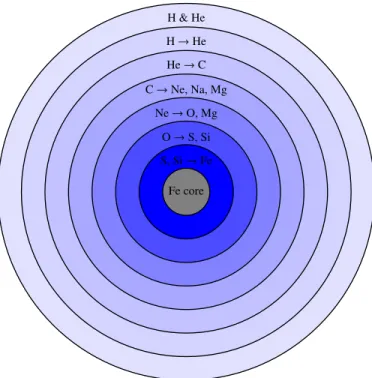
heavier elements (O, Ne, S, etc.), all the way up to 56Fe. Figure 1.6 shows the onion-like structure of the core in these massive objects, at the end of their life.
When they explode as Supernovae, part of the heavy nuclei in the core are dispersed into the interstellar space, enriching the ISM in the surroundings of the
1.4. The influence of high-mass stars on their environment 28 H & He H → He He → C C → Ne, Na, Mg Ne → O, Mg O → S, Si S, Si → Fe Fe core
Figure 1.6: Core of a massive star in the last phases of its life, before it explodes as a supernova.
dying star. Elements heavier than56Fe are created mainly through reactions of
neutron capture during the supernova event. The production of heavy elements is particularly important for the chemistry and the energetic balance of the ISM, because they are the dominant actors for the cooling of the interstellar medium. Massive stars strongly modify their surroundings, ionising the nearby gas, injecting significant amounts of energy into the ISM and mixing it through supernova explosions, winds and expanding Hii regions. High-mass stars are thus of primary importance in determining the physical-, chemical- and morphological properties of galaxies, for their evolution, and even for the evolution of the Universe itself.
Considering their potentially destructive impact on their surroundings, high-mass stars may be expected to affect star-formation activity as well.
Several scenarios were explored in the literature, starting from the classical idea of Collect& Collapse (e.g., Elmegreen 1998). The basic principle behind this mechanism is that the material around the star is swept up on the edge of an expanding Hii region, and that the mass of the collected material eventually
1.5. Outline of the thesis 29
becomes large enough to be gravitationally unstable, forming a new generation of stars. Events of triggered star formation have been observed around Hii regions in the Galaxy (e.g., Deharveng et al. 2005; Zavagno et al. 2006; Snider et al. 2009; Brand et al. 2011). The Collect & Collapse mechanism is only able to generate less-massive stars in the subsequent stellar generations, but the fraction of massive stars may be larger than in the case of spontaneous star formation (Elmegreen & Lada 1977; Walborn & Parker 1992; Deharveng & Zavagno 2011).
Another mechanism through which massive stars may induce subsequent events of star formation is the so-called radiative implosion of cores. This process may work beyond an ionisation front produced by the massive stars, which is preceded by a shock front compressing the gas. The compression of gas may induce the collapse of pre-existing condensations that would otherwise be dispersed, and may accelerate the collapse of cores that would have collapsed anyway. For typical properties of the ionisation front and of the shocked layer, the ionisation front overcomes these cores in a time comparable to the accretion timescale of low-mass stars, thus possibly halting the accretion for some of them, by photoevaporating the remaining material still available. This may influence the IMF, that would peak at even lower masses, an effect observed in some regions (e.g., Goodwin et al. 2004).
The death of a star as a supernova can also be responsible for inducing star formation, simultaneously favouring the formation of high-mass stars. This would explain the existence of OB subgroups and the coevality of the stars (cf. Zinnecker & Yorke 2007, and references therein).
Massive stars may, however, also quench the formation of successive stellar generations. For example, they can limit the final mass of the surrounding stars (as in the radiative implosion scenario), remove the remaining gas from the surrounding environment, or they can disperse or photoevaporate cores or delay their collapse (Dale et al. 2012, 2013), transferring to them energy and momentum, through radiation and winds.
All these processes seem to be at work in the regions surrounding massive stars in our Galaxy; which of them dominates depends on the specific conditions of the environment.
1.5
Outline of the thesis
In the high-mass regime the identification of different evolutionary stages is not as clear as in the low-mass regime. To understand the details of the process and test the predictions of the models one needs to understand what are the initial
1.5. Outline of the thesis 30
conditions in the clumps before the onset of high-mass star formation, and how the clump properties change with time due to the feedback of the newly-formed stars. In this thesis I use all available observational material to determine the relative age of a sample of massive clumps. I investigate the physical conditions and -properties of massive clumps in different stages of their early evolution, and the degree of CO depletion in such objects. Comparing the typical properties of the evolutionary classes we bring out the variations therein, induced by the process of high-mass star- and cluster formation in the parent clump. Having defined an evolutionary sequence in terms of physical parameters one can now use already publicly available observations to arrange a larger sample of clumps on a timeline, and then use an instrument like ALMA to study objects in a certain evolutionary phase in great detail.
I also investigate the physical properties and star formation activity in molecular material in the vicinity of a young massive cluster, that has already dispersed the clump out of which it formed.
The thesis is organised as follows. In Chapter 2, I briefly describe the concepts of Bayesian statistics used throughout this work. In Chapter 3, I select a sample of massive clumps that are in different evolutionary phases, based on their mm- and IR properties. Then, I derive the gas and dust temperature, mass and density of these clumps, and analyse the variation of these properties from quiescent clumps, without any sign of active star formation, to clumps likely hosting a ZAMS star. In the same chapter I investigate the velocity gradients in these clumps, and briefly discuss CO depletion and recent observations of several molecular species, tracers of Hot Cores and/or shocked gas, for a subsample of these clumps. In Chapter 4, I study CO depletion in some of the brightest sources in the ATLASGAL survey, investigate how it changes from dark clouds to more evolved objects, and compare its evolution to what happens in the low-mass regime. In Chapter 5, I derive the physical properties of the molecular gas in the photon-dominated region adjacent to the Hii region G353.2+0.9 in the vicinity of Pismis 24, a young, massive cluster, containing some of the most massive and hottest stars known in our Galaxy. I derive the IMF of the cluster and study the star formation activity in its surroundings. Finally, in Chapter 6, I present a short summary of the results obtained in this work.
Chapter 2
The Bayesian approach to statistics
In order to know more of the world that surrounds us, we have to observe nature, then formulate hypotheses on the laws governing it and gather data to test them. The paradigm according to which scientific theories have to confront reality was a revolution for science.
Drawing general conclusions from these data is how we make science progress. Because the data we have will always be incomplete and fragmentary, our knowl-edge of the world will necessarily be probabilistic. Statistics is the science that allows us to connect a set of data to specific problems, and to draw the general conclusions we need through statistical inference.
A well-canonised method is now at the basis of the physical sciences, resting on a few premises:
1. A theory cannot be proven to be true beyond any doubt;
2. Until a theory is proven to be false, it is assumed to be an useful representa-tion of the physical world;
3. If two or more theories can explain a phenomenon, the simplest one is to be preferred, following Ockham’s razor, unless the added complexity is justified by the data.
Two main philosophical approaches to statistics are available, based on different definitions of probability. In the following I will describe them briefly, with special attention to the Bayesian approach, used throughout this thesis.
This chapter is based on the D’Agostini (2003), Gregory (2005) and Bolstad (2007) books.
2.1. The Frequentist approach 32
2.1
The Frequentist approach
Following the frequentist approach to statistics, probability is identified with the long-run frequency of an event. The procedures are evaluated on the basis of how they perform in the long run, over all possible samples that can be drawn from a given population. In the frequentist approach parameters are fixed, but unknown constants. Because parameters are not treated as random variables, probabilistic statements cannot be made about their value, i.e. the proposition “the true value is between x and y with a probability of z” is not allowed in the frequentist approach. This can generate confusion and create a problem of interpretation. In order to explain this issue, let’s consider the following example (D’Agostini 2003): we design a simple experiment to measure a quantity, for example the length of a pen. If we repeat the experiment n times, neglecting any systematic effect, we can derive the average of the measurement results x, and the uncertainty associated with the measurement would be σ/√n, if the uncertainty associated with the single measurement is σ. The relation
µ = x ± √σ
n (2.1)
connects the true value of the length of the pen µ with the result of the experiment. Equation 2.1 merely states that:
P µ − √σ n ≤ X ≤µ + σ √ n ! = 68%, (2.2)
not increasing our knowledge about µ itself, even though this is what we seek in doing the experiment in the first place. Here X is used, because it represents a random variable, rather than the numerical value x it can assume. It is easy to see that, on the contrary, Eq. 2.2 is often interpreted as:
P x − √σ n ≤ µ ≤ x+ σ √ n ! = 68%. (2.3)
However, this does not make sense in the frequentist approach, as µ is not a random variable and thus we cannot make probabilistic statements about its value. In this case there is a clear role reversal between the true value µ, for which we are in a state of uncertainty, and the observation x, which is considered a random variable (D’Agostini 2003).
2.2. The Bayesian approach 33
U
A
B
Figure 2.1: In this case, if B is true, then also A is true. Deduction is possible.
2.2
The Bayesian approach
The Bayesian approach has a completely different philosophy: probability is
defined either as the degree of belief of an event to turn out to be true, or as a real number expressing the plausibility of a proposition A, given the truth of proposition B; the latter is at the foundation of the Bayesian statistic as an extended logic (Gregory 2005). Either of these definitions have several advantages over the frequentist one: they are completely general and can be applied to any event, independently of the possibility of repeating a measurement n times under identical conditions; it also allows the definition of the probability of the true value of a physical quantity or of an hypothesis. In fact, after a measurement, we find ourselves in a state of uncertainty about the true value of the parameter that we want to infer. The concept of probability and the interpretation of the results of an experiment in the Bayesian approach allow us to consider the parameter as a random variable, in turn giving the possibility to make probabilistic statements on the parameter itself, solving the problem of interpretation described in Sect. 2.1.
The Bayesian approach rests on the laws of probability, as they are at the heart of the statistical inference on the parameters and are used to extend logic to deal with uncertainty, as we usually do in everyday life, adjusting our beliefs about something on the basis of whether another event happened or not (Bolstad 2007). To clarify this, let’s consider the following example taken from Bolstad (2007): suppose we have two propositions, A (e.g., “I own a motorbike”) and B (e.g., “My motorbike is a Ducati”). If B is true, then A is also true, the only conclusion consistent with the given condition. Also, if one knows that A is false, one can safely affirm that B is false too. In both cases we can use deduction. Using Venn diagrams, the situation can be represented graphically as in Fig. 2.1. On the other
2.2. The Bayesian approach 34
U
A
B
Figure 2.2: In this case, deduction is not possible, and traditional logic tells us nothing of B, if we know that A is true, and viceversa.
hand, consider that I say “I don’t have a Ducati”: using traditional logic you can’t say anything about me having a motorbike or not, i.e. you can say nothing about the truth of proposition A, knowing that B is false. In the same way, if I only say that A is true, you cannot say anything about the brand of my motorbike. However, intuitively, in the first case it is less plausible that I have a motorbike, because one of the ways A could be true was removed; conversely, in the second case, the plausibility of B to be true increases, as you already know I have a motorbike. One can visualise this with the help of Fig. 2.1 and a simple numerical example. Suppose we have 20 numbers in a hat, and we have to extract one of them. Proposition A could be “a number less than or equal to 10 is extracted” and B could be “a number less than or equal to 3 is extracted”. So, the probability of A of being true is 1/2 and that of B is 3/20. However, if we know that B is false (i.e. a number larger than 3 is extracted) the probability of A to be true is just 7/17. Conversely, if we know that A is true, then the probability of B to be true is 3/10. The above example is only the simplest of the possible cases. Figure 2.2 shows a more general case: if one of the two statements A or B is true, the other can still be either true or false. With the Bayesian approach we can formalise the qualitative, intuitive variation in plausibility of the previous example, and translate the plausibility of a proposition or event into numbers, and update it on the basis of the occurrence or non-occurrence of another event. This process is called an induction.
Measures of plausibility should have some specific properties:
1. Plausibilities have to be non-negative, real numbers, and have to agree with our common sense, for example associating larger numbers to larger plausibilities.
2.2. The Bayesian approach 35
2. When the possibility exists to represent a proposition in more than one way, then all representations must be consistent and give the same plausibility. 3. In the process of evaluation, all available information must be taken into
account.
4. To equivalent states of knowledge we have to assign the same plausibility. It can be demonstrated (Cox 1946; De Finetti 1974) that all plausibilities satisfying these requirements obey the laws of probability, which are then used in the Bayesian approach to revise our beliefs, given the data. All this permits the creation of a very general theory of uncertainty, able to take into account any source of systematic or statistical error, whichever is their distribution.
2.2.1
The rules of probability and the Bayes theorem
Three axioms are at the basis of the rules of probability, important for their internal consistency: P(A) ≥ 0 for any event A; P(U)= 1 (U is the universe, cf. Figures 2.1 and 2.2); P(A ∪ B) = P(A) + P(B), if the events are disjoint. As a simple reminder, ∪ and ∩ are the operation of union and intersection between ensembles, respec-tively; ∅ is the empty set, and E is the complement of the event E. Everything that follows can be demonstrated starting from these axioms (cf. Appendix A).
P(E)= 1 − P(E); (2.4)
P(∅)= 0; (2.5)
P(A ∪ B)= P(A) + P(B) − P(A ∩ B); (2.6)
P(A ∪ B) ≥ P(A ∩ B); (2.7)
If B is a subset of A, as in Fig. 2.1, the probability of A is greater or equal than that of B:
2.2. The Bayesian approach 36
Another important definition is that of conditional probability, which is the probability of occurrence of an event A, after the occurrence of event B, indicated as P(A|B). Suppose the situation is that shown in Fig. 2.2. If we are aware that B occurred, then we are positive that B did not, implying that all that is outside B is no longer possible. This redefines a new universe, corresponding to B, that
has to obey the second axiom. Therefore P(A|B) = P(A ∩ B)/P(B), so that
P(A|B)+ P(A|B) = 1, P(B) = 1. If two events are independent P(A|B) = P(A),
and thus
P(A ∩ B)= P(A) × P(B). (2.9)
When this is no longer valid, the events are called correlated, positively or neg-atively if P(A|B) > P(A) or P(A|B) < P(A), respectively. Consider now the set of all mutually exclusive hypotheses Hi that may influence the event A. To know
what is the probability of the various Hi, given the occurrence of B is the typical
problem of any kind of measurement, i.e. to derive the probability of the causes responsible for the observed data. The frequentist approach lacks this, using an indirect approach based on confidence, which is prone to generate the problems discussed in Sect. 2.1, arbitrarily interpreting Eq. 2.2 as 2.3. This is an intuitive process, explained by D’Agostini (2003) with the dog and the hunter example: suppose that we know that a hunter goes hunting with his dog, and that there is a 50% probability to find the dog within 100 m from the hunter. What can we say about the position of the hunter if we observe the dog? Intuitively, one would say that there is a 50% probability of finding the hunter within 100 m from the dog. The answer is correct only if the hunter may be anywhere around the dog (if this is not the case, one has a case physically analogous to measurement at the edge of a physical region; cf. Example 1 in the following), and if there is no preferential direction from which the dog approaches (non-flat distribution of a physical quantity; cf. Example 2). Remaining on the dog-hunter example, suppose there is a path in the woods and the hunter moves only along this path. If we observe the dog farther than 100 m from the road, then we know that the hunter cannotbe within 100 m from the dog. Suppose now that the dog is eager to run in the woods and tends to precede the hunter. With the aid of the Bayes theorem one can easily show that the probability of finding the hunter within 100 m from the dog will, in general, be different from 50%. Physical examples of these problematic cases are described in D’Agostini (2003) and reported in the boxes at the end of the Section.
The Bayesian approach can easily take the above situations into account. To see how, let’s start from the derivation of the single tool used for inference, the
2.2. The Bayesian approach 37
Bayes theorem.
Imagine we divide the universe into N mutually exclusive hypotheses Hi. In
order to calculate the probability of the causes behind an event E, P(E|Hi), we can
rewrite Eq. 2.9 as:
P(E ∩ Hi)= P(E|Hi)P(Hi), (2.10)
and by symmetry:
P(Hi∩ E)= P(E ∩ Hi)= P(Hi|E)P(E). (2.11)
Combining equations 2.10 and 2.11:
P(E|Hi)P(Hi)= P(Hi|E)P(E), (2.12)
we derive one of the forms of the Bayes theorem P(Hi|E)=
P(E|Hi)P(Hi)
P(E) . (2.13)
Because the hypotheses are disjoint, i.e. Hi∩ Hj = ∅ and they are exhaustive, i.e.
∪iHi = U, we can write P(E)= P [ i (E ∩ Hi) = X i P(E ∩ Hi)= X i P(E|Hi)P(Hi). (2.14)
Substituting this into Eq. 2.13, we get the standard way of writing the Bayes theorem: P(Hi|E)= P(E|Hi)P(Hi) P iP(E|Hi)P(Hi) . (2.15)
In Eq. 2.15 the expression in the denominator is only a normalisation factor, so thatΣiP(Hi|E)= 1. P(E|Hi) is called likelihood and expresses the probability that
a cause produces a given effect. P(Hi|E) is the updated probability of Hi, given
the effect E, after the measurement, or posterior. Finally, P(Hi) is the initial, a
prioriprobability of the hypothesis Hi available without the data obtained with
the current experiment. This is called prior. The use of priors has been criticised as subjective, but it is important to realise that the only thing that objectivity requires in a scientific approach is that different investigators with the same state of knowledge reach the same conclusion (De Finetti 1974; Jaynes & Bretthorst
2.2. The Bayesian approach 38
Figure 2.3: Example of measurement at the edge of a physical region, e.g. the neutrino mass (see text). The dashed red line is the prior, the solid black line is the likelihood and the solid green line is the posterior. The black dashed line shows the shortest 68% interval of the posterior.
2003). Besides, the use of priors is the only natural way to include any previous knowledge in the analysis.
The set of competing hypotheses we want to assign probabilities to is called hypothesis space. After applying the Bayes theorem to all the hypotheses, we have a probability distribution function in the case of discrete quantities or a probability density function in the continuous case, in both cases abbreviated as PDF. A PDF describes our state of knowledge, or better, ignorance, about a parameter. The true value of a parameter is not distributed over the PDF, it has a definite value, but our state of uncertainty allows us to treat it as a random variable.
Practical examples of the use of the Bayes Theorem for astronomical data are shown in the following Chapters; the PDF of the quantities we are interested in is derived explicitly for simple cases in Sections 4.6.3.2, 5.2.3.8 and B.2.
The very scheme of the Bayesian approach can be seen as a model for the process of learning (Gregory 2005), being the tool that lets us update our knowledge of the physical world on the basis of the observed data. Firstly we define our state of
2.2. The Bayesian approach 39
Figure 2.4: Example of measurement of a quantity with a non-flat distribution, e.g. the energy of cosmic rays (see text). The dashed red line is the prior, the solid black line is the likelihood and the solid green line is the posterior.
knowledge, based on the available information before the experiment, formalising it into a prior; secondly we gather the new data to construct a likelihood, and finally we use the Bayes theorem to combine it with the a priori information, to revise our information about the parameter deriving a posterior. The posterior can then be used as a prior, when new data become available.
The solution of a problem in the Bayesian paradigm is usually conceptually simple. However, a major drawback for using this approach is that it could be difficult or computationally very expensive to derive the posterior, typically requiring the integration of functions with many dimensions.
The Monte Carlo Markov Chains (MCMC) methods are one of the possible solutions to this problem, trying to simulate direct drawing from a complex dis-tribution. This class of algorithms derives its name from the fact that it uses the current value of the sample to randomly generate the next one, producing a Markov Chain (Walsh 2004). A Markov chain is a system with a finite or countable number of states. It moves successively from one state to another: each transition is called a step. If the chain is in state i it will move to the next state j (which can also be
2.2. The Bayesian approach 40
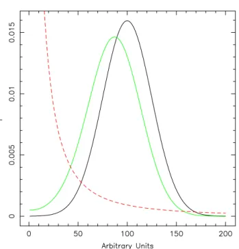
Example 1 – Measurement at the edge of a physical region. To measure the mass of the electron-neutrino, an experiment was designed, with a
resolution σ = 2 eV/c2, assumed to be independent of the mass for
simplicity. The analysis of the data from this experiment gives a neutrino mass of mν = −4 eV/c2. How is one to interpret these data? Certainly it
does not make sense to express the results in one of the following ways:
mν = −4 ± 2 eV/c2, P(−6 eV/c2 ≤ mν ≤ −2 eV/c2) = 68% or even
P(mν ≤ 0) = 98%. Figure 2.3 illustrates this situation. In the Bayesian
approach, one can interpret the experiment results as a likelihood (the black solid line), and use a prior like the red dashed line. Combining them with the Bayes theorem, we get the posterior shown as a green solid line: on this basis we can write P(mν ≤ 1.5 eV/c2) ≈ 68%.
Example 2 – Non-flat distribution of a physical quantity. Suppose that we have previous evidence that a specific quantity has a probability distribution similar to that of the red dashed line in Fig. 2.4, with low values much more probable than the high ones. This could qualitatively represent the energy of bremsstrahlung photons or of cosmic rays. We know that the probability distribution of an observable value X can be represented as a Gaussian with a certain dispersion around the true value µ, independently of its actual value. Suppose we measure x = 100, in arbitrary units. Intuitively, we expect that the true value that caused the observation has more probability to be on the left of the measured value. In Fig. 2.4 the posterior shows this, being shifted to the left. This also shows why the probability to find the hunter around the “eager” dog is no longer 50%.
the same) with a transition probability pi j. These probabilities depend only on the
actual state of the chain, and not on the previous ones.
Among the various MCMC methods, Gibbs Sampling (Geman & Geman 1984) is particularly suited for Bayesian inference, because it can be used in a very broad class of problems (Gelfand & Smith 1990). Gibbs sampling is very useful to derive posteriors (Smith & Roberts 1993), and several softwares (such as JAGS) offer an implementation of this algorithm. The power of a Gibbs sampler resides in the fact that it only needs univariate (of a single random variable) conditional distributions, that are much easier to simulate than the full joint distribution. Therefore, one simply has to simulate n random variables sequentially from their