An Accurate Mass Determination for Kepler-1655b, a Moderately Irradiated World with a Significant Volatile Envelope

THE ASTRONOMICAL JOURNAL

Journal

155

An Accurate Mass Determination for Kepler-1655b, a Moderately Irradiated World with

a Signi

ficant Volatile Envelope

Raphaëlle D. Haywood1,20 , Andrew Vanderburg1,2,20 , Annelies Mortier3 , Helen A. C. Giles4, Mercedes López-Morales1, Eric D. Lopez5, Luca Malavolta6,7 , David Charbonneau1 , Andrew Collier Cameron3, Jeffrey L. Coughlin8 , Courtney D. Dressing9,10,20 , Chantanelle Nava1, David W. Latham1 , Xavier Dumusque4 , Christophe Lovis4, Emilio Molinari11,12 , Francesco Pepe4, Alessandro Sozzetti13 , Stéphane Udry4, François Bouchy4, John A. Johnson1, Michel Mayor4, Giusi Micela14, David Phillips1, Giampaolo Piotto6,7 , Ken Rice15,16, Dimitar Sasselov1 , Damien Ségransan4,

Chris Watson17, Laura Affer14, Aldo S. Bonomo13, Lars A. Buchhave18 , David R. Ciardi19, Aldo F. Fiorenzano11, and and Avet Harutyunyan11

1

Harvard-Smithsonian Center for Astrophysics, 60 Garden Street, Cambridge, MA 01238, USA;rhaywood@cfa.harvard.edu

2

Department of Astronomy, The University of Texas at Austin, 2515 Speedway, Stop C1400, Austin, TX 78712, USA

3

Centre for Exoplanet Science, SUPA, School of Physics and Astronomy, University of St Andrews, St Andrews, KY16 9SS, UK

4_{Observatoire Astronomique de l’Université de Genève, Chemin des Maillettes 51, Sauverny, CH-1290, Switzerland} 5

NASA Goddard Space Flight Center, 8800 Greenbelt Road, Greenbelt, MD 20771, USA

6

Dipartimento di Fisica e Astronomia“Galileo Galilei,” Universita’ di Padova, Vicolo dell’Osservatorio 3, I-35122 Padova, Italy

7

INAF—Osservatorio Astronomico di Padova, Vicolo dell’Osservatorio 5, I-35122 Padova, Italy

8_{SETI Institute, 189 Bernardo Avenue, Suite 200, Mountain View, CA 94043, USA} 9

Division of Geological Planetary Sciences, California Institute of Technology, Pasadena, CA 91125, USA

10

Astronomy Department, University of California, Berkeley, CA 94720, USA

11

INAF—Fundación Galileo Galilei, Rambla José Ana Fernandez Pérez 7, E-38712 Breña Baja, Tenerife, Spain

12

INAF—Osservatorio Astronomico di Cagliari, via della Scienza 5, I-09047, Selargius, Italy

13

INAF—Osservatorio Astrofisico di Torino, via Osservatorio 20, I-10025 Pino Torinese, Italy

14

INAF—Osservatorio Astronomico di Palermo, Piazza del Parlamento 1, I-90134 Palermo, Italy

15

SUPA, Institute for Astronomy, Royal Observatory, University of Edinburgh, Blackford Hill, Edinburgh EH93HJ, UK

16

Centre for Exoplanet Science, University of Edinburgh, Edinburgh, UK

17_{Astrophysics Research Centre, School of Mathematics and Physics, Queen’s University Belfast, Belfast, BT7 1NN, UK} 18

Centre for Star and Planet Formation, Natural History Museum of Denmark, University of Copenhagen, DK-1350 Copenhagen, Denmark

19

NASA Exoplanet Science Institute, Caltech/IPAC-NExScI, 1200 East California Boulevard, Pasadena, CA 91125, USA Received 2017 July 10; revised 2018 March 16; accepted 2018 March 18; published 2018 April 20

Abstract

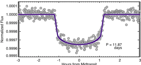
We present the confirmation of a small, moderately irradiated (F = 155 ± 7 F_⊕) Neptune with a substantial gas envelope in a P=11.8728787±0.0000085 day orbit about a quiet, Sun-like G0V star Kepler-1655. Based on our analysis of the Kepler light curve, we determined Kepler-1655b’s radius to be 2.213±0.082 R_⊕. We acquired 95 high-resolution spectra with Telescopio Nazionale Galileo/HARPS-N, enabling us to characterize the host star and determine an accurate mass for Kepler-1655b of 5.0 2.8 M

3.1

 Å via Gaussian-process regression. Our mass

determination excludes an Earth-like composition with 98% confidence. Kepler-1655bfalls on the upper edge of the evaporation valley, in the relatively sparsely occupied transition region between rocky and gas-rich planets. It is therefore part of a population of planets that we should actively seek to characterize further.

Key words: stars: individual(Kepler-1655, KOI-280, KIC 4141376, 2MASS J19064546+3912428) – planets and satellites: detection – planets and satellites: gaseous planets

1. Introduction

In our own solar system, we see a sharp transition between the inner planets, which are small(Rp„1 R⊕) and rocky, and

the outer planets that are larger (Rp… 3.88 R⊕), much more

massive, and have thick, gaseous envelopes. For exoplanets with radii intermediate to that of the Earth(1 R_⊕) and Neptune (3.88 R⊕), several factors go into determining whether planets

acquire or retain a thick gaseous envelope. Several studies have determined statistically from radius and mass determinations of exoplanets that most planets smaller than 1.6 R_⊕are rocky(i.e., they do not have large envelopes but only a thin, secondary atmosphere, if any at all; Lopez & Fortney 2014; Weiss & Marcy 2014; Dressing & Charbonneau 2015; Rogers 2015; Buchhave et al.2016; Gettel et al.2016; Lopez2017; Lopez & Rice 2016). Others have found that planets in less irradiated orbits tend to be more likely to have gaseous envelopes than

more highly irradiated planets (Hadden & Lithwick 2014; Jontof-Hutter et al. 2016). However, it is still unclear under which circumstances a planet will obtain and retain a thick gaseous envelope and how this is related to other parameters, such as stellar irradiation levels.

The characterization of the mass of a small planet in an orbit of a few days to a few months around a Sun-like star(i.e., in the incident flux range ≈1–5000 F_⊕) is primarily limited by the stellar magnetic features acting over this timescale and producing RV variations that compromise our mass determina-tions. Magneticfields produce large, dark starspots and bright faculae on the stellar photosphere. These features induce RV variations modulated by the rotation of the star and varying in amplitude as the features emerge, grow, and decay. There are two physical processes at play: (i) dark starspots and bright faculae break the Doppler balance between the approaching blueshifted stellar hemisphere and the receding redshifted half of the star (Saar & Donahue 1997; Lagrange et al. 2010; © 2018. The American Astronomical Society. All rights reserved.

20

Boisse et al.2012; Haywood et al. 2016); (ii) they inhibit the star’s convective motions, and this suppresses part of the blueshift that naturally arises from convection (Dravins et al. 1981; Meunier et al. 2010a, 2010b; Dumusque et al.2014; Haywood et al.2016).

In this paper we report the confirmation of Kepler-1655b, a mini Neptune orbiting a Sun-like star, first noted as a planet candidate(KOI-280.01) by Borucki et al. (2011). Kepler-1655b straddles the valley between the small, rocky worlds and the larger, gas-rich worlds. It is also in a moderately irradiated orbit. We present the Kepler and HARPS-N observations for this system in Section2. Based on these data sets, we determine the properties of the host star(Section3), statistically validate Kepler-1655b as a planet (Section 4), and measure Kepler-1655b’s radius (Section5) and mass (Section 6). Using these newly determined stellar and planetary parameters, we place Kepler-1655b among other exoplanets found to date and investigate the influence of incident flux on planets with thick gaseous envelopes, as compared with gas-poor, rocky planets (Section 7).

2. Observations 2.1. Kepler Photometry

Kepler-1655 was monitored with Kepler in 29.4 minutes, long-cadence mode between quarters Q0 and Q17, and in 58.9 s, short-cadence mode in quarters Q2–Q3 and Q6–Q17, covering a total time period of 1,459.49 days (BJD 2454964.51289–2456424.00183).

The simple aperture flux (SAP) shows large long-term variations on the timescale of a Kepler quarter due to differential velocity aberration, which without adequate removal obscures astrophysical stellar rotation signals as small as those expected for Kepler-1655. The Presearch Data Conditioning (PDC) reduction from Data Release 25 (DR25) did not remove these long-term trends completely due to an inadequate choice of aperture pixels. The PDC reduction from DR21, however, had a particular choice of apertures which was much more effective at removing these trends. We therefore worked with the

PDCSAP light curve from Data Release 21(Smith et al.2012; Stumpe et al. 2012, 2014) to estimate the stellar and planet parameters.

We compared the PDC(DR21) light curve with the principle component analysis(PCA) light curve and the Data Validation (DV) light curve, generated as described in Coughlin & López-Morales (2012); see also López-Morales et al. (2016) for a detailed description of these two types of analyses. All three light curves are plotted in Figure1. The PDCSAP(DR21) and PCA light curves show very similar features. They both display little variability aside from the transits of Kepler-1655b, which indicates that Kepler-1655is a quiet, low-activity star. Some larger dispersion is visible in quarters Q0–Q2, which is likely to be the signature of rotation-modulated activity(more on this in Section6.2). We note that Q12 has increased systematics in all three detrendings, possibly due to the presence of three coronal mass ejections that affected spacecraft and detector performance throughout the quarter (Van Cleve et al. 2016). The DV detrending also shows increased systematics, most likely due to the harmonic removal module in DV, which operates on a per-quarter basis(Li et al.2017).

2.2. HARPS-N Spectroscopy

We observed Kepler-1655 with the HARPS-N instrument (Cosentino et al. 2012) on the Telescopio Nazionale Galileo (TNG) at La Palma, Spain, over two seasons between 2015 June 7 and 2016 November 13. The spectra were processed using the HARPS Data Reduction System (DRS; Baranne et al. 1996). The cross-correlation was performed using a G2 spectral mask (Pepe et al. 2002). The RV measurements and the spectroscopic activity indicators are provided in Table 4. The median, minimum, and maximum signal to noise ratio of the HARPS spectra at the center of the spectral order number 50 are 51.8, 24.8, and 79.2, respectively.

The host star is fainter than typical RV targets, and its RVs can be potentially affected by moonlight contamination. We followed the procedure detailed in Malavolta et al.(2017a) and determined that none of our measurements were affected,

Figure 1.Full Q0–Q17 long-cadence Kepler light curve detrended using: Top—Presearch Data Conditioning Simple Aperture Photometry (PDCSAP, DR21); Middle—Principal Component Analysis (PCA); Bottom—Data Validation (DV). The dashed lines mark the start of each Kepler quarter.

including those carried out near the full moon. In all cases the RV of the star with respect to the observer rest frame (i.e., the difference between the systemic RV of the star and the barycentric RV correction) was higher than −25 km s−1—that is, around three times the full width at half maximum(FWHM) of the CCF—thus avoiding any moonlight contamination.

3. Stellar Properties of Kepler-1655

Kepler-1655 is a G0V star with an apparent V magnitude of 11.05±0.08, located at a distance of 230.41±28.14 pc from the Sun, according to the Gaia data release DR1 (Gaia Collaboration et al. 2016). All relevant stellar parameters can be found in Table3.

We added all individual HARPS-N spectra together and performed a spectroscopic line analysis. Equivalent widths of a list of iron lines (FeI and FeII; Sousa et al. 2011) were automatically determined using ARESv2 (Sousa et al. 2015). We then used them, along with a grid of ATLAS plane-parallel model atmospheres (Kurucz 1993), to determine the atmo-spheric parameters, assuming local thermodynamic equilibrium in the 2014 version of the MOOG code21(Sneden et al.2012). We used the iron abundance as a proxy for the metallicity. More details on the method are found in Sousa (2014) and references therein. We corrected the surface gravity resulting from this analysis to a more accurate value following Mortier et al.(2014).

We quadratically added systematic errors to our precision errors, intrinsic to our spectroscopic method. For the effective temperature, we added a systematic error of 60 K, for the surface gravity 0.1 dex, and for metallicity 0.04 dex (Sousa et al.2011).

We found an effective temperature of 6148 K and a metallicity of −0.24. These values are consistent with the values reported by Huber et al. (2013; 6134 K and −0.24, respectively), based on a spectral synthesis analysis of a TRES spectrum.

As a sanity check we also estimated the temperature and metallicity from the HARPS-N CCFs according to the method of Malavolta et al. (2017b)22 and obtained a similar result (6151±34 K, −0.27 ± 0.03, internal errors only).

The stellar mass and radius were derived using a Bayesian estimation (da Silva et al. 2006) and a set of PARSEC isochrones (Bressan et al. 2012).23 We used the effective temperature and metallicity from the spectroscopic analysis as input. We ran the analysis twice, once using the apparent V magnitude and parallax and once using the asteroseismic values Δν and νmaxobtained by Huber et al. (2013). The values are

consistent, with the ones resulting from the asteroseismology being more precise. We use the latter throughout the rest of the paper (see Table 3). These mass and radius values are also consistent with the ones obtained by Huber et al. (2013) and Silva Aguirre et al. (2015). The resulting stellar density is consistent with what is found by analysing the transit shape (see Section 5). This analysis also determined an age of 2.56±1.06 Gyr, consistent with the 3.270.640.59 Gyr from the

analysis of Silva Aguirre et al.(2015).

The spectral synthesis used by Huber et al.(2013) revealed a

vsinistarof 3.5±0.5 km s−1, making Kepler-1655 a relatively

slowly rotating star. In an asteroseismology analysis, Campante et al. (2015) determined the stellar inclination to be between 38°.4 and 90°(within the 95.4% highest posterior density credible region). This value translates into an upper limit for the rotation period of 14.8±2.4 days, and a lower limit of 9.2±2.4 days, which are consistent with the rotation period we determine from the Kepler light curve(see Section6.2).

4. Statistical Validation

The detection of a spectroscopic orbit in phase with the photometric ephemeris through RV observations is the gold standard for proving that transit signals found in Kepler data are genuine exoplanets. In the case of Kepler-1655b, however, we do not detect the planet’s reflex motion at high significance through our HARPS-N RV observations (see Section 6). Instead, in this section, we show that the transit signal is very likely a genuine exoplanet by calculating the astrophysical false positive probabilities using the open source tool vespa (Morton 2012,2015), and by interpreting additional observa-tions that are not considered by thevespa software.

Assessment of false positive probabilities using Vespa— Vespa calculates the likelihood that a transit signal is caused by a planet compared to the likelihood that the transit signal is caused by some other astrophysical phenomenon such as an eclipsing binary, either on the foreground star, or on another star in the photometric aperture.Vespa compares the shape of the observed transit to what would be expected for these different scenarios, and imposes priors based on the density of stars in thefield, constraints on other stars in the aperture from high-resolution imaging, limits on putative secondary eclipses, and differences in the depths of odd and even eclipses (to constrain scenarios where the signal is caused by an eclipsing binary with double the orbital period we find). We include as constraints two adaptive optics images acquired with the Palomar PHARO-AO system in J and K bands, downloaded from the Kepler Community Follow-up Program webpage. In the case of Kepler-1655, we also impose the constraint that we definitively rule out scenarios where Kepler-1655b is actually an eclipsing binary based on our HARPS-N RV observations, because we have a strong upper limit on the mass measurement requiring that any companion in a short period orbit be planetary.

Given these constraints, wefind a false positive probability of 2×10−3 for Kepler-1655b, which is considerably lower than the 10−2 threshold commonly used to validate Kepler candidates (Rowe et al. 2014; Morton et al. 2016). The dominant false positive scenario is that the Kepler-1655 system is a hierarchical eclipsing binary, where a physically associated low-mass eclipsing binary system near to Kepler-1655 is causing the transit signal.

Additional observational constraints—We see no evidence for the existence of a companion star to Kepler-1655according to AO imaging(see previous paragraph). The maximum peak-to-peak RV variation observed by HARPS-N is well below 20 m s−1 (see Section6). These two observational constraints entirely rule out a foreground eclipsing binary scenario. This drops the false positive probability by about a factor of 10 from the vespa estimate and thus places the false positive probability well below the threshold of 1% that is typi-cally used.

The Kepler short-cadence data, which did not go into the original vespa analysis, puts further constraints on these 21

http://www.as.utexas.edu/~chris/moog.html

22_{https://github.com/LucaMalavolta/CCFpams} 23

scenarios. The dominant scenario that arises from the vespa calculations is the hierarchical scenario. We show that this is entirely ruled out by our cadence data. With the short-cadence photometry, we resolve transit ingress and egress, measuring the duration of ingress/egress, t1,2, to be 10±

3 minutes, with ingress and egress each taking up 7%±2% of the total mid-ingress to mid-egress transit duration, t1.5,3.5. The

ratio between the transit ingress/egress time and the duration,

f=t1,2 t1.5,3.5, is a measurement of the largest possible

companion to star radius ratio, independent of the amount of blending in the light curve. If we assume that the transit is caused by a background object, the faintest background object that could cause the signal we see is only a factor of f2/(Rp/Rå)2=12±6 times fainter than Kepler-1655. For

a physically associated star, this brightness difference corresponds to roughly a late K-dwarf, with stellar radius of about 0.7 R_e. The largest physically associated object that could cause the transit shape we see is therefore about Rcompanion;0.7Re×f;6 R⊕, and therefore of planetary

size.

The last plausible scenario that remains is that of a hierarchical planet. Even though we cannot rule it out, it is a very unlikely scenario. The stringent limits on false positive scenarios from ourvespa analysis, the lack of evidence for a companion star, the fact that small planets are considerably more common than large planets, and the fact that we have a tentative detection of the spectroscopic orbit of Kepler-1655b all give us the highest confidence that Kepler-1655b is in fact a genuine planet transiting Kepler-1655.

5. Radius of Kepler-1655b from Transit Analysis Wefit the PDCSAP short-cadence light curves produced by the Kepler pipeline of Kepler-1655. Weflatten the light curve by fitting second order polynomials to the out-of-transit light curves near transits, and dividing the best-fit polynomial from the light curve. The PDCSAP short-cadence light curves have had some systematics removed, but there are still a consider-able number of discrepant data points in the light curve, especially toward the end of the original Kepler mission, when the second of four reaction wheels was close to failure. We exclude outliers from the phase-folded light curve by dividing it into bins of a few minutes. Within each of these bins, we then exclude 3-sigma outliers, although we find that a more

conservative 5-sigma clipping does not change the resulting planet parameters significantly.

We then fit the transit light curve with a transit model (Mandel & Agol 2002) using a Markov Chain Monte Carlo (MCMC) algorithm with an affine-invariant sampler (Goodman & Weare 2010). We account for the 58.34 s short-cadence integration time by oversampling model light curves by a factor of 10 and performing a trapezoidal integration. Wefit for the planetary orbital period, transit time, scaled semimajor axis (a/Rå), the planetary to stellar radius ratio (Rp/Rå), the orbital

inclination, and quadratic limb darkening parameters q1and q2,

as defined by Kipping (2013). We impose Gaussian priors on the traditional limb darkening parameters u1and u2, centered at

the values predicted by Claret & Bloemen(2011), with widths of 0.07 in each parameter (which is the typical systematic uncertainty in model limb darkening parameters found by Müller et al.2013). We sample the parameter space using an ensemble of 50 walkers, evolved for 20,000 steps. We confirm that the MCMC chains were well mixed by calculating the Gelman–Rubin convergence statistics (Gelman & Rubin1992). A binned short-cadence transit light curve and the best-fit model is shown in Figure2.

The ultra-precise Kepler short-cadence data resolves the transit ingress and egress for Kepler-1655b, and therefore is able to precisely measure the planetary impact parameter. We find that Kepler-1655b transits near the limb of its host star, with an impact parameter of 0.85 .07

.03

-+ , which makes the radius

ratio somewhat larger than would likely be inferred from afit to the long-cadence data alone (without a prior placed on the stellar density and eccentricity).

As a sanity check, we alsofit the transits of Kepler-1655b using the DV long-cadence light curve(not including quarters Q4, Q8 and Q12) using EXOFAST-1 (Eastman et al.2013).

All parameter estimatesfitted via this method are consistent with the results we obtained from our short-cadence analysis, including the eccentricity.

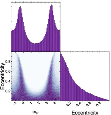
5.1. Constraint on the Eccentricity via Asterodensity Profiling We placed constraints on the eccentricity, e, and argument of periastron, ωp, of Kepler-1655b’s orbit by comparing our

measured scaled semimajor axis(a/R_å) from our short-cadence transit fits (see Section 5) and the precisely known aster-oseismic stellar parameters(listed in Table3). We followed the Figure 2.Short-cadence Kepler transit light curve of Kepler-1655b. Gray dots are the short-cadence data binned in roughly 30 s intervals. The line is the maximum-likelihood transit model.

procedure outlined by Dawson & Johnson (2012) in their Section 3.4 and explored parameter space using an MCMC analysis with affine-invariant ensemble sampling (Goodman & Weare 2010). We find that Kepler-1655b’s orbit is consistent with circular, although some solutions with high eccentricity and finely tuned arguments of periastron are allowed. Our analysis gives 68% and 95% confidence upper limits of e68%<

0.31 and e95%<0.71, respectively. The two-dimensional

probability distribution of allowed e and ωp is shown in

Figure 3. These distributions and upper limits are fully consistent with those obtained in our RV analysis (see Table3and Figure 8).

6. Mass of Kepler-1655b from RV Analysis The main obstacle to determining robust planet masses arises from the intrinsic magnetic activity of the host star.

Kepler-1655 does not present particularly high levels of magnetic activity. In fact, the magnetic behavior exhibited in its light curve, spectroscopic activity indicators, and RV curve is very similar to that of the Sun during its low-activity,“quiet” phase. However, ongoing observations of the Sun as a star show activity-induced RV variations with an rms of 1.6 m s−1, even though it is now entering the low phase of its 11 year magnetic activity cycle (Dumusque et al. 2015). More generally, several large spectroscopic surveys have shown that even the quietest stars display activity-driven RV variations of order 1–2 m s−1(e.g., the California Planet Search Isaacson & Fischer 2010; the HARPS-N Rocky Planet Search [Motalebi et al.2015]).

In the current era of confirming and characterizing planets with reflex motions of 1–2 m s−1, accounting for the effects of magnetically induced RV noise/signals, even in stars deemed to be“quiet,” becomes a necessary precaution. This is the only way we will determine planetary masses accurately and reliably (let alone precisely).

In the case of Kepler-1655, we estimate that the rotationally modulated, activity-induced RV variations have an rms of order 0.5 m s−1. Furthermore, the stellar rotation and planetary orbital periods are very close to each other, at 13 and 11 days, respectively. We perform an RV analysis based on Gaussian-process(GP) regression, which can account for low-amplitude, quasi-periodic RV variations modulated by the star’s rotation.

6.1. Preliminary Investigations

First, we perform some basic checks on the spectroscopic data available to us. We investigate whether the spectro-scopically derived activity indicators are reliable, and whether they provide any useful information for our analysis. Second, we determine the stellar rotation period and active-region evolution timescale from the PDCSAP light curve. Third, we look at the sampling strategy of the observations. In particular, we compare the two stellar timescales(rotation and evolution) to the orbital period of Kepler-1655band investigate how well all three timescales are sampled.

6.1.1.“Traditional” Spectroscopic Activity Indicators The average value of thelogRHK¢ index (−4.97) is close to

that of the Sun in its low-activity phase(≈−5.0), implying that Kepler-1655 is a relatively quiet star.

Figure 4 shows the RV observations plotted against the “traditional” spectroscopic activity indicators: the logRHK¢

index, computed from the DRS pipeline, which is a measure of the emission present in the core of the CaIIH & K lines; the FWHM and bisector span (BIS) of the cross-correlation function, which tell us about the asymmetry of the cross-correlation function(Queloz et al.2001). We see no significant correlations between the RVs and any of these activity indicators. This is expected, as they are measurements that have been averaged over the whole stellar disc, and small-scale structures such as spots and faculae, if present, are therefore likely to blur out. Moreover, the cross-correlation function is made up of many thousands of spectral lines whose shapes are all affected by stellar activity in different ways(depending on factors such as their formation depth, Landé factor, excitation potential, etc.).

Reliability of thelogRHK¢ index for this star—A recent study

by Fossati et al.(2017) found that for stars further than about 100 pc, the CaIIH & K line cores may be significantly affected by absorption from the interstellar medium (ISM), if the velocity of the ISM is close to that of the star, and the column density in the ISM cloud is high. This ISM-induced effect lowers the value of the logRHK¢ index, making the stars look

less active than they really are. Although Fossati et al.(2017) note that this effect should be stable over a timescale of years (even decades), they do caution us that it can mask the variability in the core of the CaII H & K lines and thus compromise the reliability of thelogRHK¢ index as an activity

indicator in distant stars.

Based on the parallax measurement from Gaia, Kepler-1655 is 230.41±28.14 pc away. Our line of sight to Kepler-1655 crosses three ISM clouds, labeled“LIC” (−11.49 ± 1.29 km s−1), “G” (−13.63 ± 0.97 km s−1_{), and “Mic” (−19.15 ± 1.38 km s}−1₎

in Redfield & Linsky (2008). These range from roughly 20 to 30 km s−1 redward of Kepler-1655’s barycentric velocity of −40 km s−1_{, which may lead to significant ISM absorption if the}

CaIIcolumn density in the ISM clouds(lognCaII) is high. Using

Figure 3.Correlation plots between the orbital eccentricity of Kepler-1655b and its argument of periastron. Marginalized histograms of these parameters are shown alongside the correlation plot.

the calibrations of HIcolumn density from E B( -V) of Diplas & Savage (1994) and the CaII/HI column density ratio calibration of Wakker & Mathis (2000), we deduced a column density lognCaII=12 . According to Fossati et al. (1 2017), this is on the edge of being significant. We visually inspected the CaII lines, as well as the Na D region (which often shows interstellar absorption) in our HARPS-N spectra of Kepler-1655, using the spectrum display facilities of the Data and Analysis Center for Exoplanets.24 We see two absorption features in the

Na D1 and D2 lines at velocities consistent with those of the G and Mic clouds. The stronger of the two features is likely to be associated with the G cloud, which is the furthest away from the barycentric velocity of Kepler-1655. There are no visible ISM features closer to the stellar velocity, so we conclude that we should not expect thelogRHK¢ index to be affected significantly

by ISM absorption.

6.1.2. Photometric Rotational Modulation

As can be seen in Figure 5, the Kepler light curve is generally quiet but does present occasional bursts of activity,

Figure 4.Plots of the HARPS RV variations versus the logRHK¢ index, the FWHM, and the BIS of the cross-correlation function. The Spearman correlation

coefficients for each pair of variables are given in the top right-hand corner of each panel. We find no significant correlations.

Figure 5.Autocorrelation function(ACF) analysis. Top panel: full PDCSAP light curve, including transits of Kepler-1655b. Middle panels: zoom-in on a 200 day stretch of light curve during which the star is active, and corresponding ACF(dashed line), overlaid with our MCMC fit (solid line). Bottom panels: zoom-in on a quiet 400 day stretch of the light curve, with corresponding ACF. Note that the transits were excluded for the computation of the ACFs. The dashed lines mark the start of each Kepler quarter.

24

lasting for a few stellar rotations (determined in Section 6.2). These photometric variations are likely to be the signature of a group of starspots emerging on the stellar photosphere. On the Sun, dark spots by themselves do not induce very large RV variations (of order 0.1–1 m s−1; see Lagrange et al. 2010; Haywood et al.2016). However, they are normally associated with facular regions, which induce significant RV variations via the suppression of convective blueshift (on order of the m s−1; see Meunier et al.2010a,2010b; Haywood et al.2016). Therefore, we might still expect to see some activity-driven RV variations over the span of our RV observations, which could eventually affect the reliability of our mass determination for Kepler-1655b.

6.2. Determining the Rotation Period Protand Active-region

Lifetime τevof the Host Star

We estimated the rotation period and the average lifetime of the starspots present on the stellar surface by performing an autocorrelation-based analysis on the out-of-transit PDCSAP light curve. We produced the autocorrelation function (ACF) by introducing discrete time lags, as described by Edelson & Krolik (1988), in the light curve and cross-correlating the shifted light curves with the original, unshifted curve. The ACF resembles an underdamped, simple harmonic oscillator, which we fit via an MCMC procedure. We refer the reader to Giles et al.(2017) for further detail on this technique.

The full light curve is shown in the top panel of Figure5. As discussed in Section6.1.2, Kepler-1655 is relatively quiet, and most of the light curve displays no significant rotational modulation. We initially computed the ACF of the full out-of-transit PDCSAP light curve, but found it to be flat, thus providing no useful information about the rotation period and active-region lifetime.

We then split the light curve into individual chunks according to their activity levels:

1. Active light curve: we see occasional“bursts” of activity, notably in thefirst 200 days of the light curve, which we zoom in on in the middle panel of Figure 5. This photometric variability is visible in both the PDCSAP and PCA light curves(see Figure1); the PCA light curve has a slightly higher point-to-point scatter likely as a result of a larger aperture. This “active” chunk spans several Kepler quarters, making it unlikely to be the product of quarter-to-quarter systematics. The corresp-onding ACF is shown alongside it, and our analysis results in a rotation period of 13.8±0.1 days, and an active-region lifetime of 23±8 days.

2. Quiet light curve: the bottom panels of Figure5 show a 400 day stretch of quiet photometric activity, spanning several quarters. The PCA (and DV) light curves do not display any variability either. The corresponding ACF analysis yields a rotation period of 12.7±0.1 days, and an active-region lifetime of 12.2±2.8 days.

Our rotation period estimates are in rough agreement with each other, although they do differ by more than 1-σ according to our MCMC-derived errors. Several factors are likely to be contributing to this. First and foremost, the tracers of the stellar rotation, namely the active regions on the photosphere, have finite lifetimes and are therefore imperfect tracers. An active region may appear at a given longitude and disappear after a rotation or two, only to be replaced by a different region at a

different longitude. These phase changes modulate the period of the activity-induced signal, therefore resulting in a distribution of rotation periods as opposed to a clean, well-defined period. Second, the stellar surface is likely to be dominated by different types of features when it is active and non-active (e.g., when no spots are present, we may be measuring the rotation period induced by bright faculae). In the case of the Sun, it is known that sunspots rotate slightly faster than the surrounding photosphere (see Foukal 2004 and references therein). Following different tracers could plausibly result in differing rotation periods. Third, we note that differential rotation is often invoked to explain this range in measured rotation periods. While it does have this splitting effect, it is not significantly detectable in light curves of Sun-like stars(Aigrain et al.2015).

We take the rotation period to be the average value of the estimates we obtained for the various parts of the light curve, and its 1-σ uncertainty as the difference between the highest and lowest values we obtained in order to better reflect the range of rotation rates of the stellar surface. This corresponds to a value Prot=13.6±1.4 days.

Similarly, the active-region lifetime estimate that we obtain for the quiet light curve is much shorter than that measured in the active portion. At quieter times, the largest spots(or spot groups) will be smaller and will therefore decay faster than their larger counterparts(see Giles et al.2017and Petrovay & van Driel-Gesztelyi 1997, among others). For the purpose of our RV analysis we choose the longer active-region lifetime estimate of 23±8 days. In Section 6.5.1, we show that varying this value has no significant impact on our planet mass determination.

We note that the rotation period that we measure via this ACF method is in good agreement with the forest of peaks seen in the periodogram of the light curve(see panel (a) of Figure7). These photometrically determined rotation periods fall within the range derived from the vsin and inclination measurementsi

of Kepler-1655 of(9.2–14.8)±2.4 days (see Section3). They are also in agreement with the photometric rotation period determined by McQuillan et al.(2014), of 15.78±2.12 days.

6.2.1. Sampling of the Observations

The way the observations are sampled in time can produce “ghost” signals (e.g., see Rajpaul et al.2016). Such spurious signals can significantly impact planet mass determinations, and in cases where we do not know for certain that the planet exists(i.e., we do not have transit observations), they may even result in false detections(as was the case for Alpha Cen B“b”; Rajpaul et al.2016). In the paragraphs below, we describe and implement two analytical tools—namely the window function and stacked periodograms. We use them to assess the adequacy of the cadence of the HARPS-N observations and to identify the dominant signals in the data set.

Window function—A simple and qualitatively useful diag-nostic is to plot the periodogram of the window function of the observations, as is shown in panel(d) of Figure7. It is simply the periodogram of a time series with the same time stamps as the RV observations, but with no signals or noise in the data (i.e., the RVs are set to a constant). The observed signal is the convolution of the window function with the real signal. As we might expect, we see a strong forest of peaks centered at 1 day as a result of the ground-based nature of the observations. The highest peak after 1 day is at about 42 days. We note that the

42 day aliases25of the stellar rotation period(of 13.6 days) are 20.1 and 10.3 days. This second alias is rather close to the planet’s orbital period, and so we should exercise caution. This peak around 42 days arises from the fact that past HARPS-N GTO runs have tended to be scheduled in monthly blocks. Regular monthly scheduled runs can potentially lead to trouble as RV surveys are typically geared toward Sun-like stars, which have rotation periods of about a month; the observa-tional sampling, convolved with the rotaobserva-tionally modulated activity signals of the star, will likely generate beating, spurious signals. Fortunately, Kepler-1655 has a much shorter rotation period than 1 month.

Sampling over the rotation period—We must also think about whether the time span and cadence of the observations will enable us to sample the stellar rotation cycle densely enough to reconstruct the form of the RV modulation at all phases.

The physical processes and phenomena taking place on the stellar surface undoubtedly result in signals with an intrinsic correlation structure (as opposed to random, Gaussian noise). Typically they are modulated with the stellar rotation period. The active regions evolve and change over a characteristic timescale (usually a few rotation periods), which changes the phase of the activity-induced signals. If our observations sample the stellar rotation too sparsely, we may not be able to identify these phase-changing, quasi-periodic signals, and recover their real, underlying correlation structure. In this case the signals become noise; their correlation properties may be damped or changed. The sampling may be so sparse that the correlation structure becomes lost completely, in which case the resulting noise will be best accounted for via an uncorrelated, Gaussian noise term (as was the case for Kepler-21 in López-Morales et al.2016).

We obtained 95 observations over 526 nights. This corresponds to 45 orbital cycles and approximately 37 stellar rotation cycles. The two seasons cover about 150 and 200 nights, respectively. This sampling is fairly sparse, and indeed the results of our RV fitting reflect this (Section6.5).

Stacked periodograms—Figure6shows the evolution in the Bayesian Generalized Lomb–Scargle periodograms of the RVs as we add more observations (Mortier et al. 2015; Mortier & Collier Cameron2017). After about 50 observations we begin to see clear power at the orbital period of Kepler-1655b

(11.8 days). We note that this is not the only or the most prominent feature in the periodograms. We also see several streaks of power in the region of 14–16 days. This broad range of periods, centered at the rotation period (13.6 days), is consistent with the relatively short-lived, phase-changing incoherent signatures of magnetic activity. We note that these signals are convolved with the window function of the observations, which contains many peaks ranging from about 10 to 50 days(panel (d) of Figure7).

Periodicities near 2.5 and 3.2 days—We see strong peaks in the periodograms at periods of 2.5 and 3.2 days. We computed the 99% and 99.9% false alarm probability levels via boot-strapping and found that both levels lie well above the highest peaks in the periodograms of both the RV observations and the RV residuals. These signals are therefore not statistically significant. Since we do not have any other information about their nature, we did not investigate them any further.

6.3. Choice of RV Model and Priors

In light of these preliminary investigations, we choose to stay open to the possible presence of correlated RV noise arising from Kepler-1655’s magnetic activity. We take any such variations into account via GP regression. Our approach is very similar to that of López-Morales et al.(2016). The GP is encoded by a quasi-periodic kernel of the form

k t t, exp t t 2 2 sin . 1 t t 1 2 2 2 2 2 4 2 3 h h h ¢ = - - ¢ -p h - ¢ ⎡ ⎣ ⎢ ⎢ ⎢ ⎤ ⎦ ⎥ ⎥ ⎥

(

)

The hyperparameterη1is the amplitude of the correlated noise;

η2 corresponds to the evolution timescale of features on the

stellar surface that produce activity-induced RV variations; η3

is equivalent to the stellar rotation period; and η4 gives a

measure of the level of high-frequency structure in the GP model.

η2 and η3 are constrained with Gaussian priors using the

values for the stellar rotation period and the active-region lifetime determined via the ACF analysis described in Section6.2.

We constrain η4 with a Gaussian prior centered around

0.5±0.05. This value, which is adopted based on experience from previous data sets (including CoRoT-7 Haywood et al. 2014, Kepler-78 Grunblatt et al. 2015 and Kepler-21

Figure 6.Stacked periodograms of the HARPS-N RV observations, showing the evolution of the data set as we gathered the observations. Each panel spans the following period range:(a) 2–50 days, (b) zoom-in around 2.5 days, and (c) from 10 to 20 days. The color scale, equal for all three panels, represents the periodogram power. Note that the orbital period(marked by the vertical black line) is at 11.8728787±0.0000085 days, and the stellar rotation period is 13.6±1.4 days.

25

López-Morales et al.2016), allows the RV curve to have up to two or three maxima and minima per rotation, as is typical of stellar light curves and RV curves (see Jeffers et al. 2009). Foreshortening and limb darkening act to smooth stellar photometric and RV variations, which means that a curve with more than 2–3 peaks per rotation cycle would be unphysical.

The strong constraints on the hyperparameters (particularly

4

h ) are ultimately incorporated into the likelihood of our model, and as shown in Figures 8and 9 provide a realistic fit to the activity-induced variations. We note that GP regression, despite being robust, is also extremelyflexible. Our aim is not to test how well an unconstrained GP can fit the data, but rather to constrain it to the maximum of our prior knowledge, in order to account for activity-driven signals as best as we can.

We account for the potential presence of uncorrelated, Gaussian noise by adding a termσs in quadrature to the RV

error bars provided by the DRS.

We model the orbit of Kepler-1655b as a Keplerian with free eccentricity. We adopt Gaussian priors for the orbital period and transit phase, using the best-fit values for these parameters estimated in Section5. Finally, we account for the star’s systemic velocity and the instrumental zero-point offset of the HARPS-N spectrograph with a constant term RV0. We summarize the priors

used for each free parameter of our RV model in Table1. The covariance kernel of Equation(1) is used to construct the covariance matrixK, of size n × n, where n is the number of RV observations. Each element of the covariance matrix tells us about how much each pair of RV data are correlated with each other.

Figure 7.Lomb–Scargle periodograms of (a) the Kepler PDCSAP light curve; (b) the HARPS-N RV campaign; (c) the residuals from the RV fit to the HARPS-N observations; and(d) the window function of the RV campaign. None of the peaks in the periodograms of RV observations and residuals are statistically significant (the 99% false alarm probability levels are higher than the maximum power plotted).

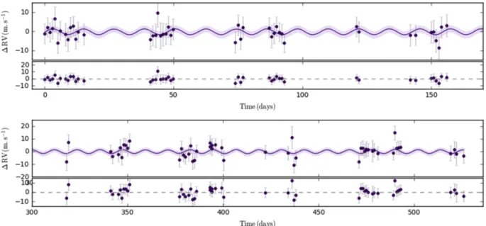
Figure 8.The HARPS-N RV data(points with error bars) and our best fit (dark line with light-shaded 1-σ error regions): (top) zoom-in on the first season; (bottom) zoom-in on the second season, the following year. The residuals after subtracting the model from the data(in m s−1) are shown in the plots below each fit.

For a data set y (with n elements yi), the likelihood  is

calculated as(Rasmussen & Williams2006)

K I K I n y y log 2log 2 1 2log 1 2 . . . 2 i T i 2 2 1  p s s = - - + - + -( ) (∣ ∣) ( ) ( )

The first term is a normalization constant. The second term, where K∣ ∣ is the determinant of the covariance matrix, acts to

penalize complex models. The third term represents theχ2of the fit. The white noise component, σi, includes the intrinsic variance

of each observation (i.e., the error bar; see Table 4) and the uncorrelated Gaussian noise term σs mentioned previously,

added together in quadrature.I is an identity matrix of size n × n. We maximize the likelihood of our model and determine the best-fit parameter values through an MCMC procedure similar to the one described in Haywood et al. (2014), in an affine-invariant framework(Goodman & Weare2010).

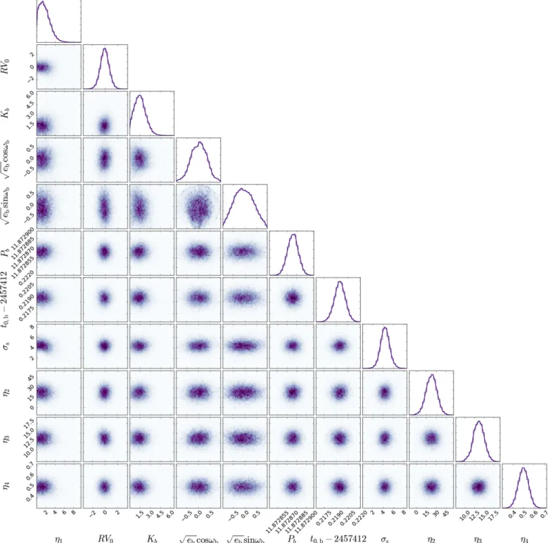
Figure 9.Marginalized 1 and 2D posterior distributions of the RV model parameters output from the MCMC procedure. The solid lines overplotted on the histograms are kernel density estimations of the marginal distributions. The smooth, Gaussian-shaped posterior distributions attest of the good convergence of the MCMC chains.

6.4. Underlying Assumptions in Our Choice of Covariance Kernel

In imposing strong priors on η2and η3, we are making the

assumption that the rotation period Prot and active-region

lifetime τev are the same in both the photometric light curve

and the RV curve. This is potentially not the case, as the photometric and spectroscopic variations may be driven by different stellar surface markers/phenomena (e.g., starspots, faculae). They may rotate at different speeds, be located at significantly different latitudes on the stellar surface, or have very different lifetimes. Faculae on the Sun persist longer than spots. They are likely the dominant contributors to the RV signal, while the shorter-lived spots will dominate the photometry.

It is difficult to check the validity of this assumption, as these very same factors also impede our ability to determine precise estimates for Prot and τev, particularly in RV observations for

which we do not benefit from long-term, high-cadence sampling. For example, the rotation period usually appears in the periodograms(of the light curve and the RVs) as a forest of peaks, rather than a single clean, sharp peak (see Figure 7). This effect is the result of the tracers (spots, faculae, etc.) having lifetimes of just a few rotations, and subsequently reappearing at different longitudes on the stellar surface. This scrambles the phase and thus modulates the period; see Section 6.2.

6.5. Results of the RV Fitting

We investigated the effect of including a GP and/or an uncorrelated noise term on the accuracy and precision of our mass determination for Kepler-1655b. We also looked at the effects of using different priors for η2and η3, and injecting a

fake planet with the density of Earth.

We tested three models accounting for both correlated and uncorrelated noise. Thefirst one, which we refer to as Model 1, contains both correlated and uncorrelated noise, in the form of a GP and a term σs added in quadrature to the errors bars,

respectively. In addition, the model has a term RV0 and a

Keplerian orbit. The second model we tested(Model 2) has no GP but does account for uncorrelated noise via a termσsadded

in quadrature to the error bars. Again, the model also has a term RV0 and a Keplerian orbit. Our third and simplest model

(Model 3) contains no noise components at all. It only contains a zero offset RV0and a Keplerian orbit.

For all models, we used the same prior values and 1-σ uncertainties for all the timescale parameters(orbital P and t0,

stellar Protandτev) as well as the structure hyperparameter η4.

We found that the eccentricity and argument of periastron remained the same in all cases(consistent with a circular orbit). The zero offset RV0was also unaffected. The best-fit values for

the remaining parameters(K, η1,σs) for each model tested are

reported in Table2.

Overall, the value of the RV semi-amplitude of Kepler-1655b is robust to within 5 cm s−1, regardless of whether we account for (un)correlated noise or not. This is a reflection of the fact that the host star has fairly low levels of activity. When the GP is included, its amplitude η1 is similar to that of K.

However, we note that the uncorrelated noise term is large and dominates both the GP and the planet Keplerian signal. This may be a combination of additional instrumental noise(the star is very faint and our observations are largely dominated by photon noise) and short-term granulation motions. Also, rotationally modulated activity signals that were sampled too sparsely may also appear to be uncorrelated and be absorbed by this term rather than the GP(as was likely the case in López-Morales et al.2016).

Regardless of its nature, we cannot ignore the presence of uncorrelated noise. Doing so would lead us to underestimating our 1-σ uncertainty on K by 40%. Finally, we see that when we go from Model 2 (uncorrelated noise only) to Model 1 (correlated and uncorrelated noise), the uncertainty on K increases by about 7 cm s−1. We attribute this slight inflation to the fact that the orbital period of Kepler-1655b is close to the rotation period of its host star. This acts to incorporate this proximity of orbital and stellar timescales in the mass determination of Kepler-1655b.

6.5.1. Effects of Varying Protandτev

We ran models with different values for the stellar rotation and evolution timescales(Protranging between 11 and 20 days,

τev ranging between 13 and 50 days, with associated

uncertainties ranging from 1 to 8 days for both). We found

Table 1

Parameters Modeled in the RV Analysis and Their Prior Probability Distributions

Orbital period(from transits) P Gaussian(11.8728787, 0.0000085) Transit ephemeris(from

transits)

t0 Gaussian(2455013.89795, 0.00069)

RV semi-amplitude K Uniform 0, ¥[ ]

Orbital eccentricity e Uniform[0, 1]

Argument of periastron ω Uniform[0, 2π]

Amplitude of covariance η1 Uniform 0, ¥[ ]

Evolution timescale (from ACF) η2 Gaussian(23, 8) Recurrence timescale (from ACF) η3 Gaussian(13.6, 1.4)

Structure parameter η4 Gaussian(0.5, 0.05)

Uncorrelated noise term σs Uniform 0, ¥[ ]

Systematic RV offset RV0 Uniform

Note.For the Gaussian priors, the terms within parentheses represent the mean and standard deviation of the distribution. The terms within square brackets stand for the lower and upper limit of the specified distribution; if no interval is given, no limits are placed.

Table 2

Effects of Including Correlated and/or Uncorrelated Noise Contributions in Our RV Fitting

K η1 σs

(m s−1_{) (m s}−1_{) (m s}−1₎

(a) Original RV data set

Model 1 1.470.800.88 1.61.01.3 4.3±0.8

Model 2 1.460.740.81 L 4.6±0.9

Model 3 1.51_0.460.47 _{L L}

(b) RV data set with injected Earth-composition Kepler-1655b

Model 1 6.130.930.90 1.81.11.3 4.40.80.9

Model 2 6.190.840.83 L 4.60.70.9

Model 3 6.25±0.48 L L

Note.Model 1: correlated and uncorrelated noise (GP, σs, RV0, and a Keplerian orbit); Model 2: uncorrelated noise (σs, RV0, and a Keplerian orbit); Model 3: no noise components(RV0and a Keplerian orbit). (b) We injected a Keplerian signal with semi-amplitude 6.2 m s−1(after subtracting the detected amplitude of 1.47 m s−1), corresponding to a mass of 22.6 M⊕.

that the amplitude of the GP and its associated uncertainty remained the same throughout our simulations. The semi-amplitude of Kepler-1655b also remained the same to within 10%, ranging between 1.37 and 1.47 m s−1, with a 1-σ uncertainty ranging from 0.85 to 0.90 m s−1. The uncertainty was largest in cases with the longest evolution timescale

composition models of Zeng et al. (2016), these mass and radius values correspond to an Earth-like composition. We tested all three Models after injecting this artificial signal. As shown in panel(b) of Table2, we see a completely consistent behavior when the semi-amplitude of the planet is artificially boosted. In particular, the amplitude η1 of the GP remains

consistent well within 1-σ. This artificial signal is detected at high significance (7-σ). This test confirms that if the planet had an Earth-like composition, our RV observations would have been sufficient to determine its mass with accuracy and precision; it therefore shows that Kepler-1655b must contain a significant fraction of volatiles. We find that only 0.014% of the samples in our actual posterior mass distribution lie at or above 22.6 M_⊕, and therefore conclude that we can significantly rule out an Earth-like composition for this planet.

6.6. Mass and Composition of Kepler-1655b

The RV fit from Model 1, which we adopt for our mass determination, is plotted in Figure 8. The corresponding correlation plots for the parameters in the MCMC run, attesting of its efficient exploration and good convergence, are shown in Figure9. The residuals, shown as a histogram in Figure11, are Gaussian-distributed. The phase-folded orbit of Kepler-1655b is shown in Figure10.

Taking the semi-amplitude obtained from Model 1, we determine the mass of Kepler-1655b to be 5.0 2.8 M

3.1

 Å. The

posterior distribution of the mass is shown in Figure12. For comparison, we also show the posterior distribution obtained after we injected the artificial signal corresponding to a Kepler-1655b with an Earth-like composition. As we discussed in Section 6.5.2, we see that the two posterior distributions are clearly distinct and with little overlap. Despite the low significance of our planet mass determination, we can state with high confidence that Kepler-1655b has a significant gaseous envelope and is not Earth-like in composition. The mass of Kepler-1655b is less than 6.2 M_⊕at 68% confidence, and less than 10.1 M_⊕ at 95% confidence. Our analysis excludes an Earth-like composition with more than 98% confidence (see Section6.5.2).

We obtain a bulk density for Kepler-1655bof r =_b 2.5 1.4 g cm

1.6 3

 - _{. The planet’s density is less than 3.2 g cm}−3

to 68% confidence and less than 5.1 g cm−3to 95% confidence. The planet may have experienced some moderate levels of evaporation, which may be significant if its mass is indeed below 5 M_⊕.

The eccentricity is consistent with a circular orbit and with the constraints derived from our asterodensity profiling analysis (Section 5.1). At an orbital period of 11.8 days, we do not expect this planet to be tidally circularized.

[Fe/H] −0.24±0.05 3 Δν[μHz] 128.8±1.3 5 νmax[μHz] 2928.0±97.0 5 Mass[Me] 1.03±0.04 6 Radius[Re] 1.03±0.02 6 ρ* [ρe] 0.94±0.04 Age[Gyr] 2.56±1.06 6 vsini(km s−1) 3.5±0.5 5 Limb darkening q1 0.403±0.077 7 Limb darkening q2 0.260±0.039 7 R log HK á ¢ ñ −4.97 8 Prot[days] 13.6±1.4 7 τev[days] 23±8 7

Transit and radial-velocity parameters

Orbital period P[days] 11.8728787±0.0000085 7

Time of mid-transit t0[BJD] 2455013.89795±0.00069 7

Radius ratio(Rb/Rå) 0.01965±0.00069 7

Orbital inclination i[deg] 87.62±0.55 7

Transit impact parameter b 0.85±0.13 7

RV semi-amplitude K[m s−1] 1.47-0.880.80 8

RV semi-amplitude 68%(95%) upper limit[m s−1]

<1.8 (<2.8) 8

Eccentricity 68%(95%) upper limit <0.36 (<0.79) 8

Argument of periastronωp[deg] −71±92 8

RV offset RV0(km s−1) −40.6386±0.000006 8

Derived parameters for Kepler-1655b

Radius Rb[R⊕] 2.213±0.082 6, 7

Mass Mb[M⊕] 5.03.1-2.8 6, 7, 8

Mass 68%(95%) upper limit [M⊕] <6.2 (<10.1) 6, 7, 8

Densityρb[g cm−1] 2.51.6-1.4 6, 7, 8

Density 68%(95%) upper limit

[g cm−1_] <3.2 (<5.1) 6, 7, 8

Scaled semimajor axis a/Rå 20.5±4.1 7

Semimajor axis ab[au] 0.103±0.001 7, 8

Incidentflux F[F⊕] 155±7 6, 7

Note.(1) Høg et al. (2000). (2) Gaia Collaboration et al. (2016). (3) From ARES+MOOG analysis, with the surface gravity corrected following Mortier et al.(2014). (4) Bayesian estimation (da Silva et al.2006) using the PARSEC isochrones(Bressan et al.2012) and V magnitude and parallax. (5) Huber et al. (2013). (6) Bayesian estimation using the PARSEC isochrones and asteroseismology.(7) Analysis of the Kepler light curve. (8) Analysis of the HARPS-N spectra/RVs.

Table 4

HARPS-N RV Observations and Spectroscopic Activity Indicators, Determined from the DRS

Barycentric Julian Date RV σRV FWHM Contrast BIS logRHK¢ slogRHK¢

[UTC] (km s−1_{) (km s}−1_{) (km s}−1_{) (km s}−1₎ 2457180.523500 −40.63968 0.00270 7.86870 29.321 0.02594 −4.9614 0.0157 2457181.527594 −40.63651 0.00236 7.86380 29.310 0.02474 −4.9651 0.0128 2457182.603785 −40.63892 0.00259 7.86953 29.305 0.02778 −4.9600 0.0147 2457183.494217 −40.63709 0.00281 7.86066 29.369 0.04133 −4.9601 0.0161 2457184.498702 −40.63199 0.00463 7.85989 29.256 0.03136 −4.9596 0.0354 2457185.495085 −40.64455 0.00293 7.87730 29.309 0.03152 −4.9532 0.0178 2457186.572836 −40.63822 0.00226 7.86260 29.343 0.02592 −4.9750 0.0118 2457188.501974 −40.64006 0.00396 7.88033 29.250 0.03398 −4.9270 0.0263 2457189.492822 −40.64273 0.00415 7.86784 29.305 0.03193 −4.9742 0.0319 2457190.506147 −40.63649 0.00296 7.85754 29.330 0.01650 −4.9878 0.0207 2457191.506484 −40.63570 0.00232 7.87102 29.344 0.02833 −4.9906 0.0132 2457192.503233 −40.64261 0.00240 7.85594 29.332 0.03865 −4.9884 0.0140 2457193.506439 −40.63887 0.00259 7.86547 29.344 0.02939 −4.9654 0.0137 2457195.618836 −40.64015 0.00320 7.85577 29.331 0.02057 −4.9571 0.0206 2457221.430559 −40.64291 0.00239 7.86913 29.361 0.02674 −4.9743 0.0133 2457222.435839 −40.64084 0.00301 7.87471 29.314 0.02747 −4.9653 0.0191 2457223.460747 −40.64063 0.00449 7.88822 29.216 0.03258 −5.0076 0.0397 2457224.390932 −40.62888 0.00576 7.86308 29.208 0.04897 −4.9174 0.0493 2457225.433813 −40.64082 0.00533 7.87820 29.198 0.02494 −5.0425 0.0564 2457226.408684 −40.64007 0.00408 7.86647 29.256 0.01841 −4.9618 0.0324 2457227.450637 −40.63983 0.00331 7.84180 29.309 0.03703 −4.9530 0.0217 2457228.410287 −40.63623 0.00341 7.87077 29.293 0.02768 −4.9568 0.0214 2457229.429739 −40.64052 0.00274 7.86533 29.298 0.03706 −4.9567 0.0156 2457230.406112 −40.63739 0.00323 7.87646 29.312 0.02833 −4.9308 0.0203 2457254.397788 −40.64424 0.00323 7.85502 29.314 0.02396 −4.9604 0.0213 2457255.500146 −40.63523 0.00299 7.86901 29.308 0.02114 −4.9755 0.0184 2457256.421107 −40.64243 0.00309 7.87620 29.285 0.02475 −5.0159 0.0213 2457257.482828 −40.63653 0.00335 7.87228 29.271 0.01542 −4.9738 0.0229 2457267.507688 −40.63665 0.00275 7.87107 29.284 0.02316 −4.9523 0.0155 2457268.565339 −40.64117 0.00391 7.87216 29.272 0.02490 −4.9535 0.0286 2457269.463909 −40.63953 0.00294 7.88436 29.297 0.02912 −4.9824 0.0188 2457270.452464 −40.63594 0.00244 7.86921 29.341 0.03088 −4.9645 0.0127 2457271.453922 −40.63895 0.00217 7.86716 29.344 0.02627 −4.9705 0.0106 2457272.495252 −40.63976 0.00269 7.87068 29.289 0.03039 −4.9893 0.0161 2457273.471826 −40.64459 0.00263 7.86265 29.320 0.03018 −4.9924 0.0149 2457301.432438 −40.63609 0.00280 7.86113 29.327 0.01631 −5.0003 0.0171 2457302.432090 −40.63881 0.00300 7.86872 29.290 0.03184 −4.9895 0.0177 2457322.359064 −40.64060 0.00339 7.86850 29.200 0.03729 −4.9534 0.0215 2457324.381964 −40.64046 0.00310 7.85083 29.271 0.03889 −4.9723 0.0192 2457330.349610 −40.63902 0.00326 7.86853 29.288 0.01826 −4.9757 0.0214 2457331.372976 −40.63873 0.00400 7.84861 29.288 0.03181 −4.9975 0.0315 2457332.370233 −40.64343 0.00392 7.88092 29.280 0.03704 −4.9701 0.0289 2457333.372096 −40.64721 0.00328 7.87162 29.263 0.02773 −5.0009 0.0246 2457334.328880 −40.63632 0.00305 7.86380 29.304 0.02669 −4.9949 0.0201 2457336.372433 −40.63546 0.00371 7.87532 29.294 0.02301 −4.9793 0.0267 2457498.664041 −40.64669 0.00518 7.85834 29.142 0.00964 −4.9501 0.0413 2457499.669841 −40.63127 0.00428 7.85774 29.202 0.02395 −4.9950 0.0349 2457521.623607 −40.63859 0.00294 7.87430 29.328 0.03426 −4.9826 0.0181 2457522.593255 −40.64256 0.00331 7.85636 29.278 0.03021 −5.0042 0.0245 2457525.643222 −40.64070 0.00368 7.85232 29.286 0.04013 −4.9688 0.0257 2457526.666772 −40.63541 0.00447 7.85574 29.270 0.02673 −4.9869 0.0360 2457527.615676 −40.64328 0.00429 7.86272 29.214 0.03598 −4.9852 0.0342 2457528.632060 −40.63341 0.00328 7.86301 29.249 0.02537 −4.9359 0.0199 2457529.644972 −40.63372 0.00324 7.86321 29.255 0.02607 −4.9483 0.0205 2457530.649803 −40.63592 0.00418 7.85874 29.177 0.02875 −5.0283 0.0366 2457531.672726 −40.63028 0.00382 7.85133 29.244 0.01415 −4.9776 0.0283 2457557.640527 −40.64505 0.00403 7.84956 29.207 0.03445 −4.9784 0.0301 2457558.611395 −40.63639 0.00426 7.83640 29.255 0.03740 −4.9370 0.0298 2457559.640215 −40.64116 0.00355 7.87551 29.164 0.02475 −4.9554 0.0227 2457560.634300 −40.64283 0.00378 7.85731 29.167 0.02360 −4.9598 0.0255 2457562.593091 −40.64033 0.00377 7.86254 29.244 0.02591 −4.9733 0.0264 2457563.620948 −40.63391 0.00427 7.87441 29.158 0.04132 −4.9638 0.0310 2457564.607576 −40.64620 0.00472 7.84112 29.226 0.02182 −4.9581 0.0359

Figure 10.Phase plot of the orbit of Kepler-1655b for the best-fit model after subtracting the Gaussian-process component.

Figure 11.Histogram of the residuals of the RVs, after subtracting Model 1 from the data. The residuals are close to Gaussian-distributed.

2457580.702970 −40.64565 0.00629 7.86485 29.182 0.02583 −4.9331 0.0533 2457602.492695 −40.63907 0.00306 7.85957 29.311 0.03089 −4.9285 0.0172 2457614.470313 −40.63970 0.00287 7.86161 29.292 0.03215 −4.9681 0.0165 2457616.518107 −40.62758 0.00751 7.84425 29.065 0.03880 −4.9471 0.0676 2457617.485597 −40.64913 0.00426 7.84666 29.192 0.03402 −4.9775 0.0325 2457618.483689 −40.64341 0.00402 7.86390 29.124 0.02040 −4.9969 0.0305 2457651.405471 −40.64647 0.00294 7.86796 29.302 0.02770 −4.9582 0.0171 2457652.404666 −40.63602 0.00277 7.87473 29.349 0.02870 −4.9674 0.0154 2457653.410155 −40.63573 0.00393 7.86262 29.305 0.02438 −4.9947 0.0298 2457654.408874 −40.63807 0.00344 7.86736 29.345 0.02750 −4.9921 0.0236 2457655.380684 −40.63649 0.00424 7.86868 29.252 0.02368 −4.9915 0.0327 2457656.400628 −40.63716 0.00251 7.85571 29.329 0.02444 −4.9617 0.0132 2457658.467841 −40.63825 0.00711 7.89902 29.261 0.02978 −5.0566 0.0775 2457659.409674 −40.63750 0.00321 7.86655 29.335 0.02576 −4.9494 0.0194 2457661.433530 −40.64007 0.00263 7.86886 29.389 0.02541 −4.9687 0.0146 2457669.401610 −40.63981 0.00268 7.87027 29.322 0.03286 −4.9664 0.0149 2457670.357039 −40.62378 0.00324 7.85478 29.319 0.02758 −4.9473 0.0196 2457671.396539 −40.63589 0.00260 7.87140 29.334 0.03001 −4.9790 0.0146 2457672.400889 −40.63547 0.00289 7.87136 29.313 0.02379 −4.9728 0.0174 2457673.332071 −40.63531 0.00276 7.86742 29.302 0.02206 −5.0001 0.0160 2457699.366303 −40.64003 0.00394 7.86373 29.291 0.03020 −4.9620 0.0266 2457701.363688 −40.63710 0.00480 7.85277 29.252 0.04106 −5.0048 0.0422 2457702.373816 −40.64049 0.00819 7.89468 29.016 0.03353 −4.8835 0.0685 2457706.345872 −40.64216 0.00357 7.87407 29.227 0.04043 −4.8960 0.0203

Note.From left to right are given: Barycentric Julian date BJD, radial-velocity RV, the estimated 1-σ uncertainty on the RV (s ), the full width at half maximumRV

(FWHM), contrast and line bisector (BIS) of the cross-correlation function (as defined in Queloz et al.2001), the CaIIactivity indicator logRHK¢ , and its 1-σ

The large uncertainty on our mass determination is not unexpected. First, the host star is fainter than typical HARPS-N targets (mV= 11.05), so our RV observations are

photon-limited. Second, the window function of the RV observations contains a number of features in the 10–50 day range (see panel (d) of Figure7and Section6.2.1), which implies that the stellar rotation period, close to 14 days, is sampled rather sparsely. Any activity-induced RV variations, which can reasonably be expected at the level of 1–2 m s−1 from suppression of convective blueshift in facular areas, will thus be sparsely sampled; this is likely to wash out their correlated nature and will result in additional uncorrelated noise—which in turn inflates the uncertainty of our mass determination.

7. Discussion: Kepler-1655b among Other Known Exoplanets

With a radius of 2.213 R_⊕and a mass less than 10.1 M_⊕(at 95% confidence), Kepler-1655b straddles the region between small, rocky worlds and larger, gas-rich worlds. Figure 13 shows the place of Kepler-1655b as a function of mass and radius, alongside other well-characterized exoplanets in the 0.1–32 M_⊕and 0.3–8 R_⊕range. The exoplanets that are shown have measured masses and were taken from the list compiled by Christiansen et al. (2017). We used radius measurements from Fulton et al. (2017) where available, or extracted them from the NASA Exoplanet Archive26 otherwise. We include the planets of the solar system, with data from the NASA Goddard Space Flight Center archive.27We overplot the planet composition models of Zeng et al.(2016).

For the purpose of the present discussion, we identify and highlight the planets that have a strong likelihood of being

gaseous(in blue) and rocky (in red). For each planet, we drew 1000 random samples from a Gaussian distribution centered at the planet mass and radius, with a width given by their associated mass and radius 1-σ uncertainties. Planets whose mass and radius determinations indicate a 96% or higher probability of lying above the 100% H2O line are colored in

blue. Planets that lie below the 100% MgSiO3line with 96%

probability or higher, and have a probability of less than 4% of lying above the 100% H2O line are colored in red. All other

planets, colored in gray, are those that do not lie on either extreme of this probability distribution(even though their mass and radius measurement uncertainties may be smaller than others that we identified as rocky or gaseous). For clarity we omitted their error bars on this plot.

We note that Kepler-1655b, shown in purple is one of these intermediate worlds.

For this discussion, we define “water worlds” as planets for which the majority of their content(75%–80% in terms of their radius) is not hydrogen. Their densities indicate that they must have a significant non-rocky component, but this component is water rather than hydrogen. They formed from solids with high mean molecular weight. We refer to planets with a radius fraction of hydrogen to core that is greater than 20% as “gaseous worlds.”

We wish to investigate how gaseous planets(lying above the water line) behave as a function of planet radius and incident flux received at the planet surface as compared to their rocky counterparts. For this purpose, we created the three plots shown in Figure 14, in which planets are again displayed as probability density distributions rather than single points with 1-σ uncertainties. For each planet, we draw 1000 random

Figure 13.Mass–radius diagram for planets in the 0.1–32 M⊕and 0.3–8 R⊕ ranges. The blue points correspond to“gas-rich” planets, while the red points represent planets that are very likely to be rocky in composition(see Section7). The planets that fall in neither category are colored in gray, and their error bars are omitted for clarity. Kepler-1655band its associated 1-σ measurement uncertainties are shown in purple.

Figure 12.Posterior distributions of the mass parameter:“actual” refers to the posterior distribution obtained whenfitting Model 1 to the actual RV data, while“like” is the distribution we obtain if we inject a planet of Earth-like composition with Kepler-1655b’s 2.2 R⊕radius. Such a planet would have a mass of≈22.6 M⊕.

26_{https://exoplanetarchive.ipac.caltech.edu}

, operated by the California Insti-tute of Technology, under contract with NASA under the Exoplanet Exploration Program.

27

https://nssdc.gsfc.nasa.gov/planetary/factsheet/, authored and curated by D. R. Williams at the NASA Goddard Space Flight Center.