D
OCTORAL
T
HESIS
K
∗
(892)
±
resonance with the ALICE
detector at LHC
Author:
Kunal G
ARGSupervisor:
Prof. Francesco R
IGGIDr. Angela B
ADALÀA thesis submitted in fulfillment of the requirements
for the degree of Doctor of Philosophy Cycle XXXI
in the
“The greatest gift of education, Korya, is the years of shelter provided when learning. Do not think to reduce that learning to facts and the utterances of presumed sages. Much of what one learns in that time is in the sphere of concord, the ways of society, the proprieties of behaviour and thought. Haut would tell you that this is another hard-won achievement of civilization: the time and safe environment in which to learn how to live. When this is destroyed, undermined or discounted, then that civilization is in trouble (1)”
Contents
List of Figures vii
List of Tables xv
Introduction 1
1 Physics of the Hot QCD matter 5
1.1 Standard Model . . . 5
1.2 Quantum Chromodynamics and QGP . . . 6
1.2.1 QCD Phase trasition . . . 9
1.2.2 Bag model and Temperature phase transition . . . 10
1.3 QGP in Big and Little Bang . . . 12
1.4 QGP as a Perfect fluid . . . 16
1.4.1 Global event properties . . . 16
1.4.2 Identified Particle pT spectra and Yield . . . 18
1.4.3 Strangeness production . . . 20
1.4.4 Anisotropic Flow . . . 24
1.5 Collective behavior in small systems . . . 25
2 Hadronic resonance production at LHC 31 2.1 Event Generators and Theoretical Models . . . 31
2.1.1 PYTHIA . . . 32
2.1.2 EPOS . . . 35
2.1.3 Parton-Hadron-String Dynamics Model . . . 38
2.2 Resonances and characterisation of hadronic phase . . . 40
2.3 Some Resonance results at LHC energies . . . 47
3 A Large Ion Collider Experiment at LHC 55 3.1 The Large Hadron Collider . . . 55
3.2 The ALICE Detector . . . 56
3.2.1 Inner Tracking System . . . 61
3.2.2 The Time Projection Chamber . . . 62
3.2.3 The Time of Flight Detector . . . 65
3.2.4 VZERO . . . 65
3.2.5 Data Acquisition (DAQ) and Trigger systems . . . 66
3.2.6 Data flow: from the Online to the Offline . . . 67
3.2.7 ALICE Offline software framework . . . 69
The AliEn Framework . . . 69
3.2.8 Event reconstruction . . . 70
3.2.10 Multiplicity Determination in pp collisions . . . 74
4 K∗0and K∗± resonance reconstruction in pp collisions 77 4.1 Signal Extraction . . . 78
4.1.1 Uncorrelated background estimate . . . 80
4.1.2 Raw Yield Extraction . . . 83
4.2 K∗± Mass Determination . . . 87
5 Measurement ofK∗(892)± production in pp collisions at 13 TeV 95 5.1 K∗± reconstruction in pp collisions . . . 95
5.1.1 Data sample and event selection . . . 95
5.1.2 Primary tracks selection . . . 96
5.1.3 Pion Identification . . . 97
5.1.4 V0selection . . . 98
5.1.5 Signal Extraction . . . 99
5.2 Monte Carlo corrections . . . 99
5.2.1 Reweighted Acceptance×Efficiency . . . 100
5.2.2 Signal-Loss correction . . . 102
5.3 Systematic Uncertainties . . . 103
5.3.1 Global tracking uncertainty . . . 103
5.3.2 Systematic due to material budget . . . 103
5.3.3 Systematic due to hadronic interactions . . . 104
5.3.4 Systematic estimation procedure using grouping method . 105 5.3.5 Consistency Check . . . 106
5.3.6 Smoothing procedure for systematic uncertainties . . . 108
5.3.7 Total systematic uncertainty . . . 110
5.4 K∗± Transverse momentum spectrum . . . 112
6 K∗0 results in pp collisions at 13 TeV 115 6.1 K∗(892)0 reconstruction in pp collisions . . . 115
6.1.1 Pion and Kaon Identification . . . 115
6.1.2 K∗0raw yield and acceptance×efficiency . . . 116
6.2 K∗0pT spectrum and comparison with K∗± . . . 117
7 Results forK∗± in pp collisions at 13 TeV 121 7.1 Energy Dependence. . . 121
7.2 Model Comparison . . . 122
7.3 Particle Ratios . . . 123
7.4 K∗+vs K∗− . . . 124
8 Multiplicity dependence ofK∗± production in pp collisions at 13 TeV 131 8.1 K∗(892)± reconstruction in in different event multiplicity classes 131 8.1.1 Event, multiplicity, track and V0 selection . . . 131
8.2 Yield Estimation . . . 132
8.3 Results for K∗±production in different charged particle multiplic-ity classes. . . 135
List of Figures
1.1 Standard Model chart. . . 6
1.2 Chiral symmetry restoration . . . 8
1.3 QCD phase diagram . . . 9
1.4 LGT results. . . 10
1.5 Little Bang . . . 13
1.6 Time evolution of heavy-ion collision . . . 14
1.7 Geometry of heavy-ion collision. . . 17
1.8 Grand canonical thermal fit to ALICE central (0-10%) Pb-Pb par-ticle production rates in collisions at√sNN = 2.76 TeV (19) . . . . 20
1.9 Feynman diagrams for the ss production in QGP: the leftmost di-agram represents a quark-antiquark annihilation, while the other three correspond to gluon fusion processes . . . 21
1.10 Time evolution of the relative strangeness to baryon density (ρs/ρb) produced in the plasma for various temperatures T, with ms = 150 MeV and αS = 0.6. The vertical line corresponds to a time of∼6 fm/c. (34) . . . 22
1.11 Observed enhancement at ALICE . . . 24
1.12 Hyperon-to-pion ratios as a function of ⟨Npart⟩, for A-A and pp collisions at LHC and RHIC energies (38). The lines mark the thermal model predictions (40) (full line) and (41) . . . 24
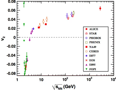
1.13 Elliptic flow observations . . . 26
1.14 3D view of the "ridge" in pp collisions . . . 27
1.15 Blast Wave Fits . . . 28
1.16 Elliptic Flow in different collision systems . . . 28
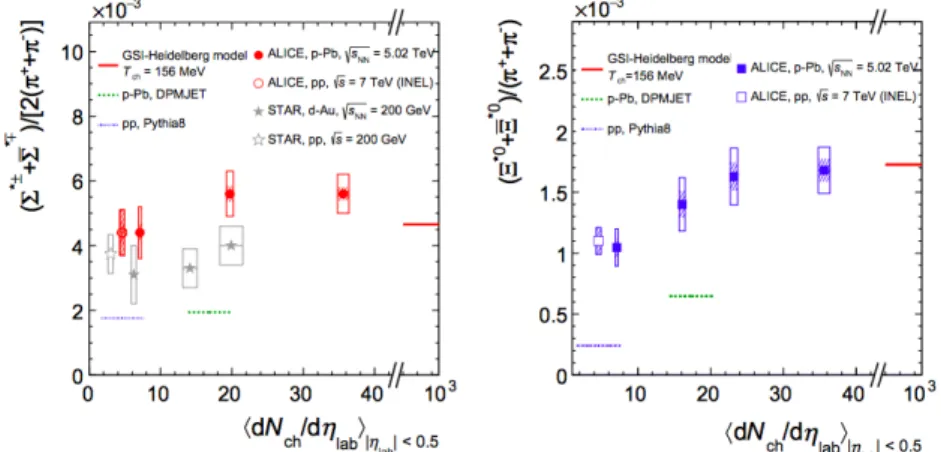
1.17 Strangeness enhancement in pp collisions . . . 29
1.18 Strangeness enhancement in pp collisions 2 . . . 30
2.1 Monte Carlo Simulations in High Energy Physics . . . 33
2.2 Proton-Proton Interaction . . . 34
2.3 Space time evolution of the particle production in a hadronic in-teraction. A hyperbola (line) represents particles with the same proper time. Figure a) is the standard approach for p-p scattering while figure b) is a more complete treatment used usually for HI collision . . . 36
2.4 Elementary interaction in the EPOS model . . . 36
2.5 Core corona picture as modelled in the EPOS . . . 38
2.6 Centrality dependence of the lifetime of the hadronic phase calcu-lated from the estimated difference in the hadronic-phase lifetime between the EPOS+UrQMD ON and EPOS+UrQMD OFF scenar-ios, calculated using hadrons (π,K,N and N). (73) . . . 38
2.7 ϕ/π and K∗0/π ratio as a function charged particle multiplicity
from pp collisions at 7 TeV (circles and thin lines), pPb at 5 TeV (squares and intermediate lines), and Pb-Pb at 2.76 TeV (stars and thick lines) (74) . . . 39
2.8 (Left)The K∗0/K− ratio as a function of the centre of mass en-ergy(CM)√sNN. Black squares and orange circles represent STAR
results for Au+Au and pp collisions, respectively. The orange cir-cle shows STAR data from pp collisions. Additionally data from the NA27 experiment are shown for lower c.m. energies as open blue diamonds. The red and green symbols show results from a PHSD calculation (78). (Right panel) K∗0/K ratio as a function of the cubic root of the charged particle multiplicity density ob-tained from the ALICE experiment compared with results from PHSD model (red stars) (79) . . . 40
2.9 The differential mass distribution dMdN for the vector kaons K∗+ + K∗0 (a, upper part) and for vector anti-kaons K∗− + K∗0 (b, lower part) for central Pb-Pb collisions at a centre-of-mass en-ergy of √sNN = 2.76 TeV at midrapidity (|y| < 0.5) from PHSD
calculations. The solid orange lines with circles show K∗’s and K∗’s reconstructed from final kaon and pion pairs while all of the other lines represent the different production channels at the de-cay point of the K∗and K∗, i.e. the black lines show the total num-ber of the K∗’s and K∗’s at their decay points, while the light blue dashed lines show the decayed K∗’s and K∗’s that stem from the
π+K annihilation and the short-dotted red lines indicate the
de-cayed K∗’s and K∗’s which have been produced during the hadro-nisation of the QGP (79). . . 41
2.10 Possible hadronic interactions between chemical and kinetic freeeze-out . . . 43
2.11 Evolution of the chemical composition of an expanding hadronic fireball produced in Au-Au collisions at√sNN= 200 GeV as
func-tion of the medium proper time, from a hydro + UrQMD model. The dark grey shaded area shows the duration of the QGP phase,
whereas the light grey shaded area depicts the coexistence phase (84). 44
2.12 Hadronic formation time as function of the particles mass M, for different quark pTand fixed fractional momentum (z). The yellow
shaded areas indicate the upper and lower limits for the medium lifetime of the partonic phase at RHIC and LHC, respectively (85). 44
2.13 ρ/π (86)(Top Left), K∗0/K and ϕ/K(Top Right) (87),Λ(1520)/Λ(Bottom
Left) (88), andΞ∗0/Ξ(Bottom Right) (88) ratios as a function of the cube root of the charged particle multiplicity density dNch/dη for
pp, p-Pb, d-Au, Au-Au, and Pb-Pb collisions . . . 45
2.14 ∆++/p (Left) andΣ∗/Λ ratios as a function of the charged particle multiplicity density dNch/dη for pp, d-Au, and Au-Au collisions
2.15 Ratios of the integrated yields, K∗0/K measured in pp collisions at √s = 7 and 13 TeV and in p-Pb collisions at √sNN = 5.02 and
8.16 TeV as a function of charged particle multiplicity (91) . . . . 47
2.16 d2N/(dydpT)distribution for ϕ(1020)(Left) and K∗(892)0(Right) as a function of pT in pp collisions at √ s =7 TeV. The results are compared to theoretical models such as PHOJET and PYTHIA (92). 48 2.17 d2N/(dydpT) distribution for Ξ(1530)(Left) and Σ(1385)(Right) as a function of pT in pp collisions at √ s =7 TeV. The results are compared to theoretical models such as PYTHIA, HERWIG, and SHERPA (93). . . 48
2.18 Differential yields of ρ0 as a function of transverse momentum in inelastic pp collisions at √s = 2.76 TeV (86). The results are compared with model calculations from PYTHIA 6 (Perugia 2011 tune) (66), PYTHIA 8.14 (Monash 2013 tune) (67) and PHOJET (94). 49 2.19 Integrated yields of ϕ (left) and K∗(892)0 (right) normalized to ⟨dNch/dη⟩ in pp collisions (at √ s = 7 and 13 TeV) and p-Pb col-lisions (at √sNN = 5.02 and 8.16 TeV) for different multiplicity classes(91) . . . 50
2.20 Mean pT distribution for various resonances, stable hadrons and hyperons as a function of charged particle multiplicity density in pp (Left) (88), p-Pb (middle) (96) and Pb-Pb collisions (Right) (88) 50 2.21 Ratios of K, K∗, p, ϕ, Λ, Ξ, and Ω to π in pp, p-Pb, and Pb-Pb collisions as a function of charged particle multiplicity density (54) 51 2.22 (Left) Ratio of Σ(1385)∗± to π± and (Right) Ratio of Ξ(1530)∗0 to π±, measured in pp, d-Au and p-Pb collisions, as a function of the average charged particle density (⟨dNch/dη⟩) measured at midrapidity. A few model predictions are also shown as lines at their appropriate abscissa (90). . . 52
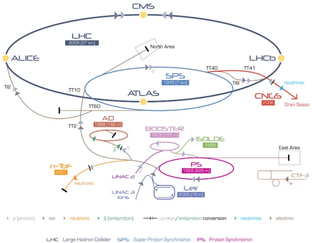
2.23 pTdifferential ratio of K∗0/K0S (left panel) and ϕ/K0S(right panel) in pp collisions at√s = 13 TeV for two different extreme multiplic-ity classes, where⟨dNch/dη⟩in high (II) and low (X) multiplicity classes are∼20 and 2.4, respectively. The bottom panel shows the ratio between the yield ratio in high to low multiplicity class (91). 53 3.1 The CERN accelerator complex . . . 57
3.2 The ALICE detector . . . 58
3.3 Cross Section of Central Barrel of ALICE. . . 58
3.4 Inner Tracking System . . . 61
3.5 dE/dx distribution of charged particles as function of their mo-mentum, both measured by the ITS alone, in pp collisions at 13 TeV. The lines are a parametrization of the detector response based on the Bethe-Bloch formula. . . 63
3.6 Momentum resolution for TPC-ITS . . . 64
3.7 Energy loss in TPC in pp collisions at√s =13TeV . . . 64
3.8 TOF β vs pTperformance plot in pp collisions at √ s = 13 TeV . . . 65
3.9 ALICE DAQ system . . . 67
3.10 ALICE Data Flow . . . 68
3.12 AliRoot framework . . . 71
3.13 ALICE track reconstruction principle . . . 73
4.1 Decay topology . . . 78
4.2 Invariant Mass Distribution Charged K* . . . 79
4.3 Invariant Mass Distribution Neutral K* . . . 80
4.4 (Left) Significance for K∗± (Right) Signal/Background ratio for K∗± . . . 80
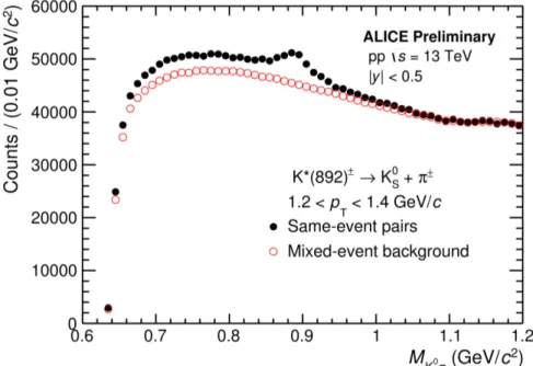
4.5 The K∓π± invariant mass distribution in|y| <0.5 in pp collisions at 13 TeV for 2.6≤pT ≤3 GeV/c from same event (black circles) and the background estimated using like-sign technique (red circles) 81 4.6 Rotated background and signal . . . 82
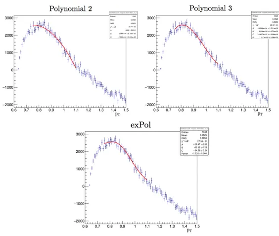
4.7 Residual background distribution for the pT bin 2.4-2.6 GeV/c ob-tained (see text) using Monte Carlo reconstructed events. Red lines represent the fit results for the three different functions: sec-ond and third order polynomial, exPol (Equation 4.4). . . 84
4.8 The K0Sπ± invariant mass distribution in|y| <0.5 in pp collisions at 13 TeV for two different pT bins after uncorrelated background subtraction. The solid red curve is the results of the fit by Equa-tion. 4.3, the dashed red line describes the residual background distribution estimated by Equation 4.4.. . . 85
4.9 The K∓π± invariant mass distribution in|y| <0.5 in pp collisions at 13 TeV for two different pT bins after uncorrelated background subtraction. The solid red curve is the results of the fit by Equa-tion. 4.3, the dashed black line describes the residual background distribution estimated by a second order polynomial. . . 85
4.10 Transverse momentum raw yield distributions estimated by bin-counting method (blue circles) and by function integration (black squares). Ratio of the two distributions (function integration/bin-counting) is shown in the lower panel. . . 87
4.11 (Left panel) The K0Sπ± invariant mass distribution in|y| <0.5 in pp collisions at 13 TeV for 6≤pT≤7 GeV/c. The solid red curve is the results of the fit by eq. 4.4, the dashed blue line describes the residual background distribution. (Right panel) Ratio of the yields obtained by the standard fit procedure (i.e fitting the dis-tribution after the uncorrelated background subtraction) and by fitting the invariant mass distribution without background sub-traction.. . . 88
4.12 RHIC Pb-Pb mass . . . 89
4.13 ALICE Pb-Pb mass . . . 90
4.14 Eff vs Mass fits . . . 91
4.15 Eff vs Mass fits . . . 92
4.16 Mass and Width vs pT (Data) . . . 92
4.17 Mass and Width vs pT (PYTHIA8) . . . 93
4.18 Mass and Width vs pT (PYTHIA6) . . . 93
5.1 Primary vertex distribution for LHCf15 data sample of 13 TeV pp collisions . . . 96
5.2 NσTPCversus momentum p estimated in the pion hypothesis
with-out any PID cut (left panel) and after p-dependent PID cut is ap-plied (right panel). The dotted lines indicate the TPC PID cuts as a function of momentum. . . 98
5.3 (Left panel) Comparison of the acceptance ×efficiency distribu-tions obtained with LHC15g3a3 (PYTHIA8), LHC15g3c3 (PYTHIA6) and LHC16d3 (EPOS-LHC) productions. (Right panel) Accep-tance×Efficiency of K∗± and K∗0 mesons as a function of pT. . . 100
5.4 Corrected K∗(892)± spectrum (black dots) with Levy-Tsallis fit (black curve). The unweighted generated (brown circles) distri-bution is compared to the reweighted one (purple crosses). The reweighted reconstructed (red crosses) and the reconstructed (green crosses) spectra are also shown. . . 101
5.5 (Left) Comparison of weighted and unweighted efficiency. (Right) Ratio of weighted and unweighted efficiency. . . 101
5.6 Comparison of signal-loss correction (ϵSL) pT distribution
esti-mated with LHC15g3a3 (PYTHIA8) and LHC15g3c3 (PYTHIA6) production . . . 102
5.7 Tracking (ITS-TPC Matching) efficiency uncertainty for K∗±. . . . 104
5.8 Material budget uncertainty pT distribution for K∗±. . . 105
5.9 (Left panel) Hadronic uncertainty pT distribution for K∗± in pp
collisions at√s = 13 TeV, estimated in the hypothesis that K0S un-certainty is equal to zero. (Right panel) Hadronic unun-certainty pT distribution for K∗± in pp collisions at
√
s = 13 TeV, estimated in the hypothesis that K0Suncertainty is equal to K+ one. . . 105
5.10 (Left) Consistency check for the number of crossed rows on pri-mary tracks. (Right) Consistency check for the cut on lifetime of K0S.. . . 109
5.11 Vmeanj pT distributions for the used cuts for primary pions
sys-tematic uncertainty estimation. The VMEANpTdistribution is also
reported. (Lower panel) The Vmeanj/VMEAN ratio as a pT function. 109
5.12 Vmeanj pT distributions for the used cuts for K
0
S systematic
uncer-tainty estimation. The VMEAN pT distribution is also reported.
(Lower panel) The Vmeanj/VMEANratio as a pTfunction. . . 110
5.13 Vmeanj pT distributions for the used cuts for Primary Vertex
sys-tematic uncertainty estimation. The VMEANpTdistribution is also
reported. (Lower panel) The Vmeanj/VMEAN ratio as a pT function. 110
5.14 The pT distributions of the systematic uncertainty of the
differ-ent sources (see text) are shown by lines of differdiffer-ent colors. The pT distribution of the total systematic uncertainty estimated for
the K∗(892)± production in pp collisions at √s = 13 TeV is also shown. . . 111
5.15 Inelastic K√ ∗(892)± spectrum at mid-rapidity in pp collisions at s = 13 TeV. Statistical (bars) and systematics (boxes) uncertain-ties are also reported. . . 113
6.2 PID for K . . . 116
6.3 Acceptance×Efficiency of K∗± and K∗0 mesons as a function of pTin pp collisions at 13 TeV . . . 117
6.4 Comparison of K∗0 spectra obtained in this thesis and in the offi-cial ALICE analysis . . . 118
6.5 INEL pT spectra of K∗± (blue points) and K∗0 (black squares)
mesons (preliminary ALICE result) as a function of pT. In the
bottom panel, ratio of K∗±/K∗0spectra is shown. . . 119
7.1 Yield for K∗0and K∗±in inelastic pp collisions at various collision energies . . . 122
7.2 K∗0(black circles) and K∗±(red squares) mean transverse momen-tum as a function of pp collision energy. Statistical and systematic uncertainties are shown by error bars and empty boxes, respectively.123
7.3 Ratios of transverse momentum spectra of K∗(892)± in inelastic pp events at√s = 8 and 13 TeV to 5.02 TeV. Statistical and system-atic uncertainties are shown by error bars and empty boxes, re-spectively. The normalisation uncertainties are shown as coloured boxes around 1 and they are not included in the point-to-point uncertainty. (130) . . . 124
7.4 Ratios of transverse momentum spectra of K∗0, ϕ, and π in inelas-tic pp collisions at√s = 5.02, 7, 8, and 13 TeV to 2.76 TeV (130) . . 125
7.5 K∗(892)± inelastic pT spectrum for pp collisions at √
s = 13 TeV compared with the pTspectrum predicted by PYTHIA8 - Monash
2013 (blue lines), PYTHIA 6 - Perugia 2011 (red lines), and EPOS-LHC (magenta lines). In the bottom panel the Data/Model ratios are reported. The gray band shows the fractional uncertainty of the measured data points. . . 126
7.6 Ratios of transverse momentum spectra of K∗± in inelastic pp collisions at√s = 8 and 13 TeV to 5.02 TeV. Predictions from diff-ferent event generators are reported. . . 127
7.7 K∗(892)±/K ratio (red circles) for pp collisions at √s = 5.02, 8, and 13 TeV compared with the K∗0/K (blue and black symbols) one for different systems and collision energies. The symbols for K∗± are slightly displaced for readability of the figure . . . 127
7.8 K∗(892)±/π ratio for pp collisions at√s = 5.02, 8, and 13 TeV com-pared with the K∗0/K one for different systems and collision en-ergies. The symbols for K∗(892)± are slightly displaced for read-ability of the figure. . . 128
7.9 Acceptance×Efficiency for K∗+vs K∗− . . . 128
7.10 Top: pT spectrum of K∗+ (blue circles) and K∗− (black squares).
Statistical uncertainties are shown as vertical lines and systematic uncertainties as bars. Bottom: Ratio of the pT spectrum K∗+/K∗−. 129
7.11 Ratio of generated K∗+/K∗− as predicted by PYTHIA6 - Perugia 2011 (left) and PYTHIA8 - Monash 2013 (right) event generator . 129
8.1 Raw pT spectra for K∗± in different charged multiplicity bins in
8.2 Ratio of acceptance × efficiency distributions in various multi-plicity bins compared to the acceptance×efficiency distribution in INEL > 0 pp collisions at 13 TeV . . . 133
8.3 K∗±Acceptance×efficiency in INEL > 0 (0-100%) pp collisions at 13 TeV . . . 133
8.4 Signal Loss correction for K∗±for different multiplicity bins in pp collisions at 13 TeV . . . 134
8.5 pTspectrum for K∗±in different charged particle mulplicity classes
in pp collisions at√s =13 TeV . . . 135
8.6 Ratio of K∗± to K∗0pTspectra in the same charged particle
multi-plicity classes . . . 136
8.7 Ratios of the K∗± pT spectra in different charged particle
multi-plicity classes to the full INEL > 0 spectrum in pp collisions at
√
s = 13 TeV . . . 136
8.8 (Top) pTspectra of K∗0 mesons in pp collisions at 13 TeV in V0M
multiplicity event classes. (Bottom) Also shown are the ratios of these pT spectra to the full 0-100% (INEL>0) pTspectrum.. . . . 137
8.9 (Left) dN/dy and (Right) ⟨pT⟩ as a function of charged particle
multiplicity density for K∗± in pp collisions at 13 TeV . . . 137
8.10 K∗±/K and K∗0/K ratio as a function of charged particle multi-plicity density in pp collisions at√s =13 TeV . . . 138
List of Tables
2.1 Properties of hadronic resonances: lifetime (τ), quark composi-tion, hadronic decay used to identify them with its branching ra-tio (%)) (81). . . 42
4.1 K∗0and K∗± properties (81) . . . 77
5.1 Standard and modified cuts for primary pion identification. . . . 107
5.2 Standard and modified cuts for secondary tracks and K0S identifi-cation.. . . 107
5.3 Standard and modified cuts for primary vertex identification. . . 107
5.4 Standard and modified parameters for signal extraction. . . 108
5.5 Main sources and weighted values of the relative systematic un-certainties (expressed in %) of the differential yield of K∗(892)± res-onance for low, intermediate and high pT ranges. . . 111
5.6 The pT integrated(K∗++K∗−)/2) yield dN/dy|y|<0.5, the mean
transverse momentum,⟨pT⟩pp collisions at √
s = 13 TeV. The first error represents the statistical uncertainty and the second one is the systematic uncertainty. . . 113
8.1 Correction factor ( fNorm) for event normalisation in each charged
Introduction
The thesis reports a measurement of K∗(892)±in pp collisions at√s = 13 TeV. In particular the transverse momentum spectrum has been measured in inelastic pp collisions and in different multiplicity classes. The K∗(892)0production has been studied at the same energy and compared with the charged resonance pro-duction.
Quantum ChromoDynamics (QCD), the theory of strong interactions, is well known in the perturbative regime, while it is not fully understood in the non-perturbative domain, where the generation of the hadronic matter and the quark confinement should be described. The gluon self-coupling is responsible for the asymptotic freedom of the interaction and confinement. QCD predicts that the strong coupling strength decreases with increasing energy or momentum trans-fer, and vanishes at asymptotically high energies. The observation of Higgs boson has been able to explain how elementary particles attain mass through Yukawa coupling and spontaneous symmetry breaking, but the quarks only ac-count for about 5 % of the hadronic mass, that instead is generated dynami-cally by strong interaction inside the hadrons. The state of matter where quarks are deconfined and chiral symmetry is restored, named Quark-Gluon-Plasma (QGP), predicted on the basis of thermodynamical considerations and QCD cal-culations, has been observed in heavy ion collisions at the RHIC and LHC ener-gies. This state of matter should be present after the electro-weak phase transi-tion, about 1µs after the Big Bang. Then with a phase transition the initial decon-fined partons plasma would have reached the hadronic phase. The study of the QGP phase and QCD phase transition is therefore necessary to solve the open puzzle of the onset of confinement and the hadron masses. This is done exper-imentally with ultra-relativistic heavy-ion collisions, where the energy density and temperature reached may be sufficient to form the QGP. Though recently, hints of collective effects or of features typical of ultrarelativistic heavy-ion col-lisions (such as enhancement of strangeness production) have begun to be ob-served in high multiplicity pp collisions as well.
The measurement of the production of strange resonances in ultrarelativistic proton-proton collisions permits characterisation of the global properties of the collisions and to probe strangeness production. Furthermore it helps in un-derstanding hadron production processes and in improving the description of hadronisation of strange particles in event generators such as PYTHIA, EPOS-LHC. Additionally the measurement of resonances over a large transverse mo-mentum range and at different collision energies permits to probe the perturba-tive (hard) and the non-perturbaperturba-tive (soft) QCD processes. Hadronic resonances are also important probes of the hadronic phase of the medium formed during
the heavy-ion collisions. K∗(892)± and K∗(892)0are strange vector mesons with a lifetime of∼ 4 fm/c, comparable to the fireball produced in heavy ion colli-sions. Thus it is expected that regeneration and rescattering processes occurring during the hadronic phase should modify the measured K∗± and K∗0 meson yields. Measurements in inelastic pp collisions constitute a reference for the study in larger colliding systems and a benchmark of the existing hadronisation models in elementary collisions, while measurements in pp collisions at high multiplicity should test the characteristics of the QCD matter formed in these collisions.
This thesis is divided in eight chapters.
Chapter1 The general physics context, with an introduction to QCD and the connection with the idea of the QGP, obtained at high density and tem-perature, is given in this first chapter. In addition a general description of the fundamental characteristics of heavy-ion collision and the time evo-lution of the created system are presented. Some new interesting results observed in small systems as a function of the event multiplicity will be also presented.
Chapter2 In this chapter the importance of the resonances for the characteri-sation of the hadronic phase will be discussed. Some of the main results recently observed will be presented. Strange hadron production in pp col-lisions is a key to understand strangeness production and hadronisation. Some of the main event generators and models as (PYTHIA, EPOS-LHC, PHSD) will be described
Chapter3 In this chapter the detection capabilities of the ALICE apparatus are given with specific focus on Time Projection Chamber (TPC), Time of Flight Detector (TOF), and Inner Tracking System (ITS). Moreover, the details on the different steps necessary to convert the electronic signals from the de-tectors into data suitable for analysis are presented.
Chapter4 The methods used to estimate the raw yields for K∗0 and K∗± is de-scribed. The measurement of the K∗± characteristics such as mass and width is also described.
Chapters5 Measurement of the transverse momentum spectrum of K∗± and of its yield in inelastic pp collisions at√s = 13 TeV is described in this chapter. Chapter6 Measurement of the K∗0 transverse momentum spectrum in pp col-lisions at 13 TeV and its comparison with the charged K∗ results are dis-cussed here.
Chapter7 Main physics results obtained with the measurement of the K∗±pT
spec-trum in inelastic pp collisions at 13 TeV. In particular, comparison with other collision energies, ratios with other particles (such as pion and Kaon) are discussed. Furthermore comparison with PYTHIA8, PYTHA6, EPOS-LHC event generators are presented. Transverse momentum spectra for
K∗+ and K∗−, separately and prediction from event generators are also discussed.
Chapter8 K∗± results as a function of event charged particle multiplicity are presented here. In particular, pTspectrum,⟨pT⟩, dN/dy, and ratio to kaons
in different multiplicity classes are presented and compared to the same observables measured for K∗0at the same collision energy.
Chapter 1
Physics of the Hot QCD matter
1.1
Standard Model
Since the advent of Quantum Mechanics (2) in 1920s, the subsequent theories, and discoveries have resulted in a remarkable insight into the fundamental struc-ture of matter. We have discovered that everything in the universe is built from some basic fundamental building blocks called elementary particles and four fundamental forces that govern their interactions. The Standard Model (SM) of particle physics is the theory describing three of the four known fundamental forces (the electromagnetic, weak, and strong interactions, and not including the gravitational force) in the universe, as well as classifying all known elemen-tary particles. The Standard Model was developed in 1970s and since then has passed every experimental test thrown its way with astonishing accuracy. There are seventeen particles in the standard model, organised into the Figure1.1. The last particles discovered were the W and Z bosons in 1983 (3), the top quark in 1995 (4), the tau neutrino in 2000 (5), and the Higgs boson in 2012 (6).
All elementary particles depending on their spin are separated into either bosons or fermions. These are differentiated via the spin-statistics theorem of quantum statistics. Particles of integer spin exhibit Bose-Einstein statistics and are bosons. Particles of half-integer spin exhibit Fermi-Dirac statistics and are fermions. They also follow the Pauli exclusion principle. This states that two fermions may not be described by the same quantum numbers. There are twelve fermions and five bosons in the standard models.
The mathematical formulation of the SM is quite complex. The information has been encoded into a single Lagrangian which can be compactified into a four line version as: L = −1 4FµνF µν +i ¯ψDψ+h.c. +ψ¯iyijψjϕ+h.c. + |Dµϕ|2−V(ϕ)
FIGURE1.1: Standard Model chart
Here,Lis defined such that the Lagrangian L is its integral over density space. The term−1/4FµνFµν is the scalar product of the field strength tensor Fµν
con-taining the mathematical encoding of all interaction particles except the Higgs boson, where µ and ν are Lorentz indices representing the spacetime compo-nents. The term i ¯ψ̸ Dψ describes how interaction particles interact with matter
particles. The fields ψ and ¯ψ describe (anti)quarks and (anti)leptons. The bar
over ¯ψmeans that the corresponding vector must be transposed and
complex-conjugated; a technical trick to ensure that the Lagrangian density remains scalar and real. ̸D is the so-called covariant derivative, featuring all the interaction particles (except the Higgs), but this time without self-interactions. The term
ψiyijψjϕdescribes how matter particles couple to the Brout-Englert-Higgs field ϕand thereby obtain mass. The entries of the Yukawa matrix yij represent the
coupling parameters to the Brout-Englert-Higgs field, and hence are directly re-lated to the mass of the particle in question. These parameters are not predicted by theory, but have been determined experimentally. The term|Dµϕ|2describes
how the interaction particles couple to the BEH field. This applies only to the interaction particles of the weak interaction, which thereby obtain their mass. And lastly, the term−V(ϕ)describes the potential of the BEH field. Contrary to
the other quantum fields, this potential does not have a single minimum at zero but has an infinite set of different minima.
1.2
Quantum Chromodynamics and QGP
Soon after the discovery of atomic nucleus, existence of a binding force hold-ing together the nucleons in the nuclei was postulated to assure nucleus stabil-ity. This was termed as the strong nuclear force (1934). The discovery of neu-tron (7) and later of pion (8) started to provider a rather satisfactory picture of
the nucleus with the pion recognised as the long searched Yukawa particle of the strong interaction. This early picture turned out to be too simplistic soon as new particles were being discovered in new experiments. The idea of protons with constituent particles, quarks began to emerge. Deep inelastic experiments shed further light on the nucleonic structure, and properties of the strong in-teraction. The quarks exist in six different flavours and carry strong "colour" charge in three different types. The "mediators" of the strong force, playing the same role of the photon for electromagnetism, are called gluons, which come in eight colour combinations. The major difference between gluons and pho-tons comes from self-interaction which leads to two following properties of the "colour force":
Colour confinement: Quarks are always observed in a colourless combinations inside hadrons, and never as free quarks.
Asymptotic freedom: the value of the strong coupling constant, αS, depends on
the momentum transfer (Q2) at which an observed process occurs (running cou-pling constant). αS decreases with increasing energy and asymptotically, at
infi-nite energy, goes to zero.
Another aspect which is important when discussing the strong force is the mass of the hadrons. Sum of constituent quarks of most hadrons made up of the three lightest quarks, is only a small fraction of the actual hadron mass. For instance, the proton (uud) mass is 1 GeV/c2while the sum of the bare masses of its constituent quarks is about 25 MeV/c2. The explanation for this phenomenon is accomplished by a process named "Chiral symmetry breaking".
Chiral symmetry breaking
The interaction of quarks and gluons is described with a gauge field theory called "Quantum Chromodynamics" (QCD) in a manner very similar to what QED does for electrons and photons. In both cases, we have spinor matter fields interacting through massless vector gauge fields. In QCD however, the intrinsic colour charge is associated with the non-Abelian gauge group SU(3), in place of the Abelian group U(1) for the electric charge in QED. As a result, quarks carry three colour charges, and gluons carry eight combinations of these colour charges. Gluon as a result becomes self-interactive, in contrast to an ideal gas of photons. The three dimensional Laplace equation, which in non relativistic QED approximated to Coulomb potential (V ∝ 1/r); for massive quarks becomes ef-fectively one dimensional, with the confining potential (V ∝ r) as a solution. The Lagrangian density of QCD is given by:
L = −1 4F a µνF µν a +
∑
f ψaf(iγµDµ)ψ f β (1.1)with the non-Abelian group tensor
Fµνa = (∂µAνa−∂νAaν−g f a
bcAbµA
c
and Dµ =∂µ+ig λa 2 A a µ (1.3)
The fundamental degrees of freedom of the theory are the 3×6 quark fermionic fields ψ, and the eight gluonic fields Aµ. λa and fbca are the eight SU(3) group
generators (the 3×3 Gell-Mann matrices) and structure constants. In the defini-tion above, the ψ represents for each flavour, a vector (ψred; ψgreen; ψblue) of the
fermionic fields. Since they are based on non-Abelian symmetry group, interac-tion terms between the vector bosons of the theory, the gluons, are present. The inclusion of quark mass adds a Lm term to the Equation1.1.
Lm =
∑
fmfψ f
aψf a (1.4)
If the mass term is neglected, the QCD Lagrangian in the Equation 1.1 be-comes chirally symmetric i.e. invariant under separate flavour rotations of the right and left-handed quarks. Neglecting the mass term is a good approxima-tion for the very light up and down quarks and a reasonable approximaapproxima-tion for strange quarks. The non-zero vacuum expectation value of the scalar quark den-sity operator ψψ breaks this symmetry and leads to a dynamic mass of the order 300 MeV for the up and down quarks and about 450 MeV for the strange quarks. A pictorial view of the spontaneous chiral symmetry breaking mechanism can be seen in the Figure1.2.
FIGURE1.2: Pictorial view of the spontaneous breaking of the
chi-ral symmetry. The quark, represented by the sphere, tends to oc-cupy the minimum energy state: in the left configuration, it corre-spond to a symmetric state; in the right configuration, representing the confined quark in a nucleon, the parton is forced to break the
1.2.1
QCD Phase trasition
Strongly interacting matter can exist in different phases characterised by a given temperature and densities, as summarised in the QCD phase diagram (see Fig-ure1.3) where temperature versus baryo-chemical potential µB is reported. The
baryo-chemical potential is defined as the energy needed to increase by one unity, the total number of baryons and anti-baryons in a system (NB),
µB =∂E/∂NB
and it is introduced to consider that at relativistic energies, the particle num-ber in a system may not be conserved due to particle annihilation and creation processes at microscopic level. In this diagram, standard nuclear matter is rep-resented at low temperatures and low µB. By increasing the temperature or the
potential, the hadronic gas (HG) is attained. At a given temperature and poten-tial, a new phase of matter, the Quark Gluon plasma should exist. In this phase, the quarks are no longer confined in hadrons and the chiral symmetry should be partially restored.
FIGURE1.3: Phase diagram of the QCD (9)
Lattice studies of QCD thermodynamics have provided quantitative infor-mation on the QCD phase transition, the equation of state and many other as-pects of QCD thermodynamics. Lattice QCD (LQCD) tells us (10) that for zero net baryon density, QCD matter undergoes a phase transition at Tcr = 173±15
MeV from a colour-confined hadron resonance gas (HG) to a colour-deconfined quark-gluon plasma (QGP). The critical energy density ecr ≃0.7 GeV/fm3
cor-responds roughly to that in the centre of a proton. At the phase transition, the normalised energy density e/T4 rises rapidly by about an order of magnitude
over a narrow temperature interval ∆T ≲ 15 - 20 MeV, whereas the pressure p/T4is continuous and rises more gradually (see Figure1.4)
FIGURE1.4: The normalized energy density ϵ/T4 (left) and
pres-sure p/T4(right) from lattice QCD for 0, 2 and 3 light quark flavors,
as well as for 2 light + 1 heavier (strange) quark flavors. Horizontal arrows on the right indicate the corresponding Stefan-Boltzmann
values for a non-interacting quark-gluon gas.(10)
Results shown in Figure1.4were obtained from Lattice Gauge Theory (LGT) for a different number of dynamical fermions. The energy density exhibits the typical behaviour of a system with a phase transition: an abrupt change in a very narrow temperature range. The corresponding pressure curve shows a smooth change with temperature. In the region below Tc, the basic constituents of QCD,
quarks and gluons, are confined within hadrons and here the EoS is well param-eterised by a hadron resonance gas. Above Tc the system appears in the QGP
phase where quarks and gluons can travel distances that substantially exceed the typical size of hadrons.
1.2.2
Bag model and Temperature phase transition
Lack of a satisfactory theory to understand the confinement leads to many phe-nomenological models. Some of these attempts, though they lack a proper link with QCD equations, are quite successful in the predictions of hadronic prop-erties. Prominent among them are the bag models (11). Motivated by field theoretical investigations, one can assume that the physical vacuum which is the "normal phase" outside hadrons, cannot support the propagation of quark and gluon fields. In such a vacuum, a small domain of different phase may be formed. It is like boiling the vacuum and creating small bubbles with a char-acteristic hadron size. Inside the bubble, quark and gluon fields can propagate freely. Hadrons are then pictured as small domain in the new phase with quark and gluon as constituents. This is the bag and the boundary surface of the bag between the two phases is impermeable against the colour fields, therefore they can’t penetrate into the normal phase of the vacuum. The impermeability at the surface is expressed in the form of boundary conditions for the colour fields. The gluon electric fields Ei (i = 1,2. . . , 8) in an octet of eight colours are tangential
whereas the gluon induction fields Bi are normal to the surface in the
energy or momentum flux through the surface. The dynamics of the quark and gluon fields inside the bag is governed locally by the field equations of quan-tum chromodynamics (QCD). Gluons are confined inside the hadron phase and quarks become also confined. Apart from the feature of the fully relativistic for-mulation, the most important new element in the bag model is that hadrons are described as deformable droplets whose shapes are determined dynamically. In the naive bag model, hadrons are considered as spherical bag and the quarks are Dirac particles permanently confined within the volume of the bag which has a finite radius equal to that of the hadron size. The assumption that the quarks move freely inside the cavity tries to imitate the basic property of asymp-totic freedom. A typical ingredient in the bag model is the small u and d quark masses (∼10 MeV). This kind of bag Model has a Lorentz scalar term for con-finement supplemented by a bag pressure (B) to prevent expansion. The bag potential acts on the mass of the quark or gluon which become very heavy at the surface of the bag and hence cannot escape. The pressure exerted by the gluon fields on the boundary of a hadron is balanced by volume energy B per unit volume and a surface energy per unit surface. The boundary of the bag is transparent against leptons and the mediators of electromagnetic and weak in-teractions.
In the bag model, the mass of a hadron increases roughly in proportion to the to-tal number of quarks inside the bag. This is due to the fact that the quark kinetic energy dominates the total energy of the bag. This would imply that multiquark hadrons are heavier than three quark bags. However, if one takes into account the one gluon exchange interaction between the quarks, the mass of the hadron in the bag model is given by:
M(R) = N×2.04 R + 4πR3B 3 ∓ N×0.117 R αs+ Z0 R (1.5)
Here first term is just the Kinetic Energy of the N quarks in a spherical bag of radius R where N = 3 for baryons and N = 2 for mesons. Second term is the extra energy required to keep the bag stable, third term is the hyperfine interaction due to the one gluon exchange, the last term corresponds to all other effects which are difficult to account for, such as the centre of mass correction, the zero point energy, self energy etc. In the static spherical model, the pressure balance equation is equivalent to minimisation of M(R) as a function of R. Thus, for equilibrium at R=Rh(Rh =radius of the hadron),
∂M(R) ∂R |R=Rh =0 provides B= 1 4π αh R4h (1.6) where
αh= (2.04±0.117αs+Z0/N)N (1.7)
N is the number of quarks constituting the hadron. Substituting the equilib-rium condition in Equation1.5, we get
MN = 16 3 BR 3N (1.8) = 4 3 αN RN (1.9) With the typical bag model parameters, B1/4 = 145 MeV, Z0 = -1.84, αs = 2.2
and the strange quark mass = 279 MeV, the masses of the lowest baryon octet and decuplet as well as the lowest meson octets are reasonably well explained except the pion mass.
Moving further into the model, a transition is expected when the free gas pres-sure of the quarks/gluons exceeds the bag prespres-sure: Pf reegas ≥B. Now
PQGP =dQGPπ2T4/90
where dQGPis the degrees of freedom for QGP and is composed of two parts:
dQGP =dg+7/8dq+q =16+7/8.6Nf2
where dgis the degrees of freedom for gluons and dq+qis the degrees of freedom
for quarks. Ideally, number of quark flavours (Nf =3) for 3 massless quarks, but
since the strange quark mass is not negligible compared to up an down quarks, an approximate value of Nf = 2.5 is taken. Thus we get dQGP = 37. This leads
to
37π2T4/90≥ B⇒Tc ≃ ( 90
37π2)
1/4B1/4
Giving us a critical temp Tc =145 MeV if bag pressure is taken to be 200 MeV.
1.3
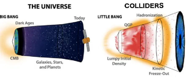
QGP in Big and Little Bang
A commonly quoted goal of the heavy-ion programs at Brookhaven Lab (BNL) and CERN, is to recreate conditions similar to those shortly after the Big Bang (about 10 µs) when the universe was filled with a quark-gluon plasma (QGP). There is now considerable evidence that the universe began as a fireball, the so called "Big-Bang", with extremely high temperature and high energy density (see left panel of Figure 1.5). At early enough times, the temperature was cer-tainly high enough (T>100 GeV) that all the known particles (including quarks, leptons, gluons, photons, Higgs bosons, W and Z) were extremely relativistic. Even the "strongly interacting" particles, like quarks and gluons, would inter-act fairly weakly due to asymptotic freedom and perturbation theory should be
sufficient to describe them. Thus this was a system of hot, weakly interacting colour charged particles, a quark-gluon plasma, in equilibrium with the other species.
QGP can be created by smashing heavy nuclei together at relativistic speeds in collisions called "little bangs" (see right panel of Figure1.5). Heavy ion collisions at the LHC and at RHIC create macroscopic (compared to the relevant micro-scopic length scale given by the inverse temperature) amounts of QCD matter. Studying the properties of this "QCD condensed matter" through an active in-teraction between theory and experiments allows us to gain unique insights to the behaviour of the strong interaction.
FIGURE 1.5: Schematic of the expansion of the universe after the
Big Bang (left) and the expansion of a fireball after Little Bang (right)
Figure1.6(12) summarises the key stages of relativistic heavy-ion collisions: thermalisation, expansion, and decoupling. In the very early collision stages, a pre-equilibrium phase is present where, "hard" particles with either a large mass or large transverse momenta pT ≫1 GeV/c are created. Their creation involves
large momentum transfers Q2∼p2 >1 GeV/c. Then these ’hard probes’ can be used to inspect the initial stages of the collisions and as hard scattering processes can be treated under perturbative QCD (pQCD). According to the uncertainty relation hard particle production happens on a time scale τf orm ≃ 1/
√
Q2; for
a 2 GeV particle this means τf orm ≃ 0.1 fm/c. In nucleus-nucleus collisions, the
quanta created in the primary collisions between the incoming nucleons can’t right away escape into the surrounding vacuum, but re-scatter of each other. In this way they create a form of dense, strongly interacting matter which ther-malises quickly and at sufficiently large energy density, forms a quark-gluon plasma. Thus with heavy-ion collisions, there is a possibility to recreate the mat-ter in the state that existed in the very early universe.
The plasma formed lives for a very short amount of time (about 10 fm/c) and during this time undergoes a rapid expansion in space into the vacuum sur-rounding the collision. As a consequence of collective expansion, the fireball
FIGURE1.6: Stages of a relativistic heavy-ion collision and relevant
theoretical concepts. (12)
cools and its energy density decreases. When the latter reaches the critical value of about 1 GeV/fm3, the hadronisation takes place. The volume of the system expands as energy density decreases (to account for entropy) by a large fac-tor in a small amount of time while the temperature remains approximately constant. This is the moment (called "chemical" freeze-out) where the particle abundances are fixed. Generally, the freeze-out moment (the end of a statisti-cal system) is defined as a moment when hadrons cease to interact and start to stream freely to detectors. It is possible to distinguish two freeze-out: the chem-ical and the kinetic freeze-out. The first corresponds to the moment when the inelastic interactions between hadrons cease and the chemical composition of the system is fixed. The thermal (kinetic) freeze-out corresponds to the moment
when elastic interactions also cease and hadrons start to escape freely. Then the created hadronic medium after the chemical freeze-out keeps expanding and hadrons keep interacting quasi-elastically, cooling the system until the "kine-matic" freeze-out is reached. At kinetic freeze-out all hadrons (including res-onances) have an approximately exponential transverse momentum spectrum reflecting the temperature of the fireball at that point. The unstable resonances can decay producing daughter particles with a smaller transverse momenta on an average than their stable counterparts.
There are various probes which can help us in studying the interactions and properties of the formed QCD matter:
− Kinematic probes and chemical composition: The multiplicities, yields, momentum spectra and correlations of hadrons emerging from heavy-ion collisions at pT < 1.5 GeV/c, reflect the properties of the bulk of the matter
produced in the collision
− Electromagnetic probes: Spectral shape of thermal radiation emitted by the QGP via qq annihilation should provide a direct measurement of the plasma temperature
− Strangeness enhancement: Strange particles are of particular interest since the initial strangeness content of the colliding nuclei is very small and there is no net strangeness. Since the focus of this thesis is a strange resonance, this signature will be discussed in detail later in this chapter
− Charmonium and Bottomonium suppression: The initially formed cc or bb pair would be unable to form a resonance in a QGP medium because of the colour screening due to the free quarks
− High-pTand jet suppression: When a high-energy parton traverses a length
L (dimension of the coloured medium) of hot or cold matter, the induced radiative energy loss is proportional to L2. The energy loss of a high-energy jet in a hot QCD plasma appears to be much larger than in cold nuclear matter. This is termed as "jet quenching"
− Elliptic Flow: It is the azimuthal momentum space anisotropy of particle emission from non-central heavy-ion collisions in the plane transverse to the beam direction. It directly reflects the initial spatial anisotropy of the nuclear overlap region in the transverse plane and since spatial anisotropy is largest at the beginning of the evolution, elliptic flow is especially sensi-tive to the early stages of system evolution
Depending on the phase of the collision, there are two probes:
− hard probes are signals produced in the first stages of the collision by the interaction of high momentum partons, such as, production of heavy quarks and of their bound states (charmonium and bottomonium), jet quench-ing, thermal photons and dileptons
− soft probes are signals produced in the later stage of the collision. Even if they are produced during the hadronisation stage, they keep indirect infor-mation on the properties of the phase transition and on the QGP. These are momentum spectra, strangeness enhancement, anisotropic flow, particle correlations and fluctuations
In both models, the description of the transition from hydrodynamic fluid to free particles which reach the detector is done using the Cooper-Frye freeze-out picture (13). In this picture it is assumed that the momentum distribution of the final state particles is essentially the momentum distribution within the fluid, towards the end of the hydrodynamical expansion, and parts of the fluid are instantaneously converted into free particles
1.4
QGP as a Perfect fluid
Such a phase of matter, named the Quark-Gluon Plasma (QGP), where the de-grees of freedom are quarks and gluons, can be created by colliding heavy ions at the RHIC and LHC energies. Its detailed characterisation should provide in-sight into the unexplained features of QCD that are crucial for understanding hadron and nuclear properties.
The most important results obtained at RHIC before LHC are:
1. the saturation of the elliptic flow v2reaching the maximum value possible
for an ideal liquid with vanishing shear viscosity (14)
2. the suppression of high pTparticles, caused by energy loss or "jet
quench-ing" in the hot and dense matter (15)
These two results established that the in heavy ion collisions the state of hot, dense matter is created. This matter is quite different and even more remarkable than had been predicted. The new state of matter created in the ion collisions is more like a liquid than a gas. Now the standard model of the ion physics is the sQGP, i.e. strongly interacting (almost) perfect liquid. These effects then have been confirmed by the observations at LHC at even higher energies. In the fol-lowing some results on soft particle production, including particle abundances and collective flow will be presented.
1.4.1
Global event properties
Heavy-ion nuclei when accelerated to ultra-relativistic energies, are Lorentz con-tracted into pancakes while travelling along the beam axis (z-axis). In a way, their collisions can be assumed to be a superposition of binary nucleons-nucleon collisions. Since not all collisions are head on, there are nucleons that partici-pate (called "participants") and those which do not interact (called "spectators") as seen in the Figure 1.7. However, a participant nucleon from the projectile can interact with multiple nucleons from the target. The number of participant-participant interactions is called the number of binary collisions, Ncoll.
FIGURE1.7: Ultra-relativistic heavy ions collision as seen from the yz plane (left) and transverse (xy) plane (right). b is the impact pa-rameter.ΨRis the reaction plane angle and ϕ the general azimuthal
angle
The impact parameter b is defined as the vector between the centres of the two nuclei in the transverse plane and quantifies the overlap region of the col-liding nuclei. Smaller the value of b, more the number of participants and the collision is more head-on. Centrality is one of the main parameters that are used to characterise the collisions. In general, centrality is directly related to the im-pact parameter b. In practice, the centrality is estimated from the multiplicity assuming that dNch/dη is monotonically increasing with Npart (i.e. as the
col-lision becomes more central). The highest centrality events then also yield the highest multiplicities. Parameters like Npartand Ncollare extracted by a Glauber
Monte Carlo simulation (16).
The impact parameter vector is important for the determination of the event plane of the collision, defined by the angle ΨR between the beam direction (z
axis) and the impact parameter vector, as depicted in Figure1.7. Particle pro-duction in the final state is normally defined in terms of new variables rapidity (y) and pseudo-rapidity(η). Rapidity (y) is defined as :
y= 1
2ln
E+pL
E−pL
where E is the particle energy and pL is its longitudinal momentum i.e. the
component of the momentum along the beam axis. The other two components of the momentum are combined as transverse momentum pT =
√ p2
x+p2y.
In composite particle collisions such as protons or nucleons, only pT
conser-vation can be applied since distribution of momentum along the longitudinal axis amongst various participants cannot be quantified, as opposed to electron-positron collision. The rapidity can be approximated by pseudo-rapidity in the ultra-relativistic limit, E≃p:
η = 1 2ln p+pL p−pL = −ln [ tanθ 2 ]
with θ being the angle of the particle momentum with respect to the z axis. The particles produced with high transverse momentum (pT) in hard scattering
pro-cesses also have η∼0.
The most basic quantity, and indeed the one measured within days of the first
ion collisions, is the number of charged particles produced per unit of (pseudo)rapidity, dN/dy (dNch/dη), in a central collision. The value finally measured at LHC in
Pb-Pb collisions at √sNN = 2.76 TeV was dNch/dη ∼1600 (17). From the
mea-sured multiplicity one can derive a rough estimate of the energy density with the help of the formula proposed by Bjorken (18) which relates the initial energy density ϵ to the transverse energy ET:
ϵ ≥ dET/dη
τ0πR2 =3/2⟨ET/N⟩
dNch/dη
τ0πR2 (1.10)
where τ0denotes the thermalisation time, R is the nuclear radius, and ET/N ∼
1 GeV is the transverse energy per emitted particle. The value measured at the LHC implies that the initial energy density (at τ0 =1 fm/c) is about 15 GeV/fm3,
approximately a factor three higher than in Au+Au collisions at the top energy of RHIC. The corresponding initial temperature increases by at least 30%, with respect to RHIC, to T∼ 300 MeV, even with the conservative assumption that the form at on time τ0, when thermal equilibrium is first established, remains
the same as at RHIC. .
1.4.2
Identified Particle
p
Tspectra and Yield
The level of equilibrium in produced particles can be tested by analysing the par-ticle abundances or their momentum spectra. The earlier is established through the chemical composition of the system, while the latter extracts additional in-formation about the dynamical evolution and collective flow. The particle pro-duction (π, K, p,Λ, ..) is a non-perturbative process and cannot be calculated directly from first principles (QCD). In the phenomenological QCD inspired event generators, the particle spectra and ratios are adjusted to the data of el-ementary collisions (pp, e+e−) using a large number of parameters. In heavy ion reactions, however, inclusive particle ratios and spectra at low transverse momentum (about 95% of all particles are below 1.5 GeV/c at LHC energies), are consistent with simple descriptions by statistical/thermal (19) and hydrody-namical models (20).
In particular particle ratios are determined during hadronisation at or close to the QGP phase boundary ("chemical freeze-out"), while particle momentum spectra reflect the conditions somewhat later in the collision, during the "ther-mal freeze-out".
The expansion of the hadrons emitted in Pb-Pb collisions is characterised by the appearance of collective flow in the soft region of the spectrum. Collective flow
implies a strong correlation between position and momentum variables and arises in a strongly interacting medium in the presence of local pressure gradi-ents. Collective motion can be studied in the framework of hydrodynamic mod-els, where the momentum spectra and the motion patterns are determined by the fluid properties (viscosity, equation of state, speed of sound) and the bound-ary conditions in the initial and in the final state (collision geometry, pressure gradients, freeze-out conditions). Radial flow is the component of the collective motion isotropic (or angle averaged) with respect to the reaction plane. It deter-mines the expansion in the radial direction and can be estimated by measuring the primary hadron transverse momentum (pT) spectra.
The average radial flow velocity (⟨βT⟩) and kinetic freeze-out temperature (Tkin,
temperature when the hadrons cease to interact) can be estimated by fitting si-multaneously the π, K and p spectra with a hydrodynamic-inspired function, called a Blast Wave (21). For the most central Pb-Pb collisions at √sNN = 2.76
TeV, ALICE (17) measures Tkin ∼95 MeV and⟨βT⟩= 0.66c, which corresponds
to a value about 10% higher than the one measured by STAR (22). Similar value has been extracted also in most central Pb-Pb collisions at√sNN= 5.02 TeV (23).
Hadron multiplicities and their correlations are observables which can provide information on the nature, composition, and size of the medium from which they originate. Of particular interest is the extent to which the measured par-ticle yields approach equilibrium. The chemical freeze-out is the moment, in the evolution of the heavy-ion collisions at which all inelastic collisions between particles cease. The chemical composition is fixed at this point.
The application of statistical concepts to multi-particle production in high en-ergy collisions was first done by Fermi in 1950s (24) and then further strength-ened by Hagedorn in 60s (25). Hagedorn was also able to explain the almost universal slope of pT spectra in his renowned statistical bootstrap model,
as-suming that resonances are made of hadrons and resonances in turn. In these models multiple hadron production proceeds from highly excited regions emit-ting hadrons according to a pure statistical law.
In modern view, the statistical or thermodynamical models are model of hadro-nisation , describing the process of hadron formation at the scale where QCD is no longer perturbative. The basic quantity required to compute the ther-mal composition of particle yields is the partition function Z(T,V). In the Grand Canonical (GC) ensemble:
ZGC(T, V, µQ) = Tr[e−β(H−∑iµQiQi)] (1.11)
where H is the Hamiltonian of the system, Qiare the conserved charges and µQi are the chemical potentials that guarantee that the charges Qiare conserved on the average in the whole system. Finally β=1/T is the inverse temperature. It is observed that the bulk hadron yields in heavy-ion collisions are well de-scribed in the framework of thermal (statistical) hadronisation models (26),(27). In these models particles are created in thermal (phase space) equilibrium, with two relevant parameters the chemical freeze-out temperature Tchemand the
baryo-chemical potential µB (which accounts for baryon number conservation). The
An additional strangeness saturation parameter, γsis introduced to describe the
observation that in some collision systems particles containing strange quarks are suppressed compared to the grand canonical thermal expectation. This pa-rameter has the value of about 1 at RHIC and LHC energies. Statistical models are able to successfully describe almost all bulk hadron yields, from centre of mass energies of a few GeV to a few TeV (28), (29). The Tchem extracted from
thermal and statistical model fits to the data is close to the phase transition temperature obtained from recent lattice calculations and is found to saturate from RHIC to LHC energies, where heavy-ions collide at an order of magnitude higher centre of mass energy.
In particular for recent central (0-10%) Pb-Pb collisions at 5.02 TeV (30), T≈152
± 3 MeV has been observed at µB =0, while a value of T ≈156 MeV at µB =
0 has been obtained for Pb-Pb collisions (0-10% centrality) at 2.76 TeV (19). In Figure1.8are reported the particle production rates measured by ALICE in cen-tral (0-10%) Pb-Pb collisions at√sNN = 2.76 TeV with a grand canonical thermal
fit. It is interesting to note as at 2.76 TeV, yields of light flavour hadrons are qualitatively well described by equilibrium thermal models over seven orders of magnitude.
In a large system with a large number of produced particles, the conservation law of a quantum number (e.g. strangeness) can be implemented on the aver-age by using the corresponding chemical potential, within the Grand Canonical formulation. In a small system, such as a pp collision, with small particle mul-tiplicity, conservation laws must be implemented locally on an event-by-event basis, requiring a Canonical formulation (C). The C conservation of quantum numbers is known to severely reduce the phase space available for particle pro-duction. This is the canonical suppression (CS) mechanism (31).
FIGURE1.8: Grand canonical thermal fit to ALICE central (0-10%)
Pb-Pb particle production rates in collisions at√sNN= 2.76 TeV (19)
1.4.3
Strangeness production
The enhancement of strange quark production, relative to light u and d quarks, in heavy ion collisions, respect to the corresponding signals from elementary re-actions, proposed by Johann Rafelski and Berndt Müller (32), has been among the first signals for probing the Quark Gluon Plasma formation. Indeed, in QGP
the production of a strange - antistrange quark pair can proceed as described in Figure1.9by the fusion of two gluons or massless light quarks. The reaction threshold in the second case is twice the mass of the produced ss pair, which due also to the partial chiral restoration is equal to the naked strange quarks, i.e. 2× 100 = 200 MeV. Moreover in QGP the equilibration of strangeness is more efficient due to the large gluon density. Then the production of multi-strange baryons could be enhanced during the deconfined phase due to recombination mechanisms. An enhanced production of hyperons is therefore expected to be a signal of a deconfined phase.
FIGURE1.9: Feynman diagrams for the ss production in QGP: the
leftmost diagram represents a quark-antiquark annihilation, while the other three correspond to gluon fusion processes
QCD matter can exists in two different phases::
1. Hadron Gas: (HG) where the degrees of freedom are the hadronic ones, as quarks and gluons are confined;
2. Quark Gluon Plasma: (QGP) where the degrees of freedom are the par-tonic ones, with quarks and gluons free with respect to each other.
The difference of the production rates of the strange quark in the two systems has been discussed on the basis of the "Reaction threshold" and " Equilibration time " (33).
Reaction threshold:
The energy needed to produce strange mesons or baryons in a thermally equi-librated HG is significantly higher than in the case of a QGP. In HG, there is an abundance of pions hence the production π+π → π+π+strange hadron +
antiparticle, should be dominant. However it is penalised due to the baryon and strange number conservation thus it is necessary to produce strange particle and antiparticle jointly. Then the reaction threshold corresponds to two times the rest mass of the hadrons: 2230 MeV for theΛ+Λ, 2642 MeV for the Ξ−+Ξ+, 3344 MeV for theΩ−+Ω+. A lower threshold is obtained in the case of indirect pro-duction. In this case multi-strange hadrons will be created in a reaction chain. First the production of lighter hadrons (π+N →K+Λ) followed by a reaction
(π+Λ → K+Ξ and π+Ξ → K+Ω). In this case the combined threshold for
Ω production is (535 + 565 + 710) MeV = 1810 MeV.
In the QGP the gluon density is high and provides the possibility to have strange quark production from gluon fusion processes as depicted in the three right
Feynman diagrams of Figure 1.9. These become the dominant processes, pro-ducing 80% of the ss pairs. In these reactions the energy threshold, due also to the partial chiral symmetry restoration, is equal to the naked mass of the two strange quarks≃2×100 MeV
Equilibration time:
The second important point is that the equilibration times in QGP, especially due to gluon fusion processes are much shorter those of the hadronic reactions. Difference is more pronounced in case of multi-strange baryons due to their low hadronic cross sections. In a partonic scenario, with a typical temperature of T = 200 MeV, equilibration times of τQGPeq ∼ 10 fm/c are theoretically achievable in an ideal gas of quarks and gluons (32) which is of the order of the expected total duration of a heavy-ion reaction, from the first parton collisions to the final freeze-out of the hadrons. Figure1.10 shows the time evolution of the relative strangeness to baryon density
FIGURE1.10: Time evolution of the relative strangeness to baryon
density (ρs/ρb) produced in the plasma for various temperatures T,
with ms= 150 MeV and αS= 0.6. The vertical line corresponds to a
time of∼6 fm/c. (34)
Following these arguments, production of multi-strange particles in HG is much more difficult as compared to QGP. In a QGP, the production probability depends on the density of the strange quarks to the power of number of strange quarks inside a hadron. The following relations are obtained in light of these arguments:
Ω/Ξ(QGP) ≈ Ξ/Λ(QGP) (1.12) Ω/Ξ(HG) <Ξ/Λ(HG) (1.13) Ω/Ξ(QGP) > Ω/Ξ(HG) (1.14) Ξ/Λ(QGP) >Ξ/Λ(HG) (1.15)