View of Statistical Methods in Phylogenetic and Evolutionary Inferences

(1)

STATISTICAL METHODS IN PHYLOGENETIC AND

EVOLUTIONARY INFERENCES

Luigi Bertolotti

Department of Animal Productions, Epidemiology and Ecology, and Molecular Biotechnology Center, University of Torino, Italy.

Mario Giacobini

Department of Animal Productions, Epidemiology and Ecology, Faculty of Veterinary Medicine, and Molecular Biotechnology Center, University of Torino, Italy.

1. PREFACE

Molecular instruments are the most accurate methods in organisms’ identification and characterization. Biologists are often involved in studies where information about ge-netic features of organisms is fundamental and where the main goal is to identify re-lationships among individuals. In this framework, it is very important to know and apply the most robust approaches to infer correctly these relationships, allowing the right conclusions about phylogeny.

Together with the establishment of new molecular techniques, scientists developed a large number of different methods to compare individuals basing on differences among them. In his book, Joseph Felsenstein (2004) provides a very good and deep explanation of these techniques, together with a detailed description of phylogenetic tree building methods.

This review will introduce the reader to the most used statistical methods in phy-logenetic analyses, the Maximum Likelihood and the Bayesian approaches, considering for simplicity only analyses regarding DNA sequences.

In the first section we will introduce the concept of the Maximum Likelihood and we will apply it the phylogenetic trees, including models of molecular evolution and explaining how to draw a tree. In the next section we will move on Bayesian statistics applied to phylogenetic inferences: we will introduce the a posteriori concept and we will describe how to create tree topology using the Metropolis Markov chains Mon-tecarlo algoriths. Finally, we will show several examples of studies conducted to infer about the evolution of pathogens.

(2)

Proposed by R. A. Fisher (1912), the most common method used to infer phylogeny is the maximum likelihood (ML). In this section a brief introduction to ML estimation shall be provided and its application to identify the best tree topology will be described. Considering that the majority of biologists does not exactly know likelihood, it is very important to introduce here some basic concepts. Given some data D and a hypothesis H, the likelihood of that data is given by

L_D= P (D|H ) (1)

which is the probability of obtaining D given H. In the context of molecular phylo-genetic, D is the set of sequences being compared and H is the tree topology. Thus, the problem becomes to find the likelihood of obtaining the observed sequences given a particular tree, and the goal to find the most probable outcome or, in other words, the tree showing the maximum likelihood. Maximum likelihood estimation requires three elements: a model of sequence evolution, a tree and the sequences. Briefly, model of molecular evolution are basically substitution probability matrices that indicate the probability of change from a state i to a state j at given site. In other words, consider-ing genetic sequences, models of molecular evolution must define the probability, at a nucleotide position, from a nucleotide to mutate into another nucleotide (see Table 1).

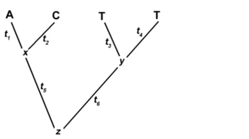
Note that a phylogenetic tree (see Figure 1) depicts both the topology (order of nodes and branches) and the branch lengths. The ML approach must solve two prob-lems: first, for a given topology, what set of branch lengths makes the observed data most likely. Second, which tree among all possible trees has the greatest likelihood.

Assuming that the evolution in different sites on a given tree is independent, the likelihood can be decomposed into the product of the probabilities at each site:

L = P (D|H ) = m Y

i =1

P (Di|τ) (2)

where Di is the data at the it hsite and τ is the tree topology. Given a tree topology, the likelihood of that tree for a site is the sum, over all possible nucleotides that may have existed at the internal nodes of the tree, of the probabilities of each scenario of events. As example, given the topology reported in Figure 1, the likelihood of each site Di of

(3)

Figure 1 – Example tree with branch lengths and data at a single site.

the tree is given by:

P (D_i|τ) = X x X y X z P (A, C , G, T, x, y, z|τ) (3) where x, y and z are the internal nodes. Assuming that differences among lineages are independent, equation 3 can be decomposed into the following product of terms:

Given a model of sequence evolution, the expression still looks difficult to compute, even if single probabilities are not hard to calculate. Problems can arise when we con-sider real data, where a large number of sequences, including a large number of sites, are considered. For each site, 43₌_{64 terms have to be considered, but on a tree with} n individuals there are n − 1 internal nodes. So we need 4n−1_{terms: for n = 10 this is} 262,144, while for n = 20 it is 274,877,906,944.

It easy to understand that the exhaustive application of this method is very hard: there are several methods (Felsenstein (1973, 1981); Gonnet et al. (1996)) to economize the computational effort but they will be not faced in this paper.

3. BAYESIANAPPROACH TOPHYLOGENY

Bayesian methods are closely related to likelihood methods, differing only in the use of a prior distribution of the variables to infer on, which would typically be the tree. In this way it is possible to interpret the results as the distributions of the variable values given the data. The use of Markov Chains Monte Carlo (MCMC) methods has recently made possible the application of Bayes’ theorem Barnard and Bayes (1958); Price (1763) to phylogenetic analyses. In this section a brief introduction to Bayes’ theorem will be proposed, together with its application to the search of the best tree topology, using Metropolis algorithms and MCMC methods.

(4)

• P (D|H ) is the conditional probability of D given H (likelihood);

• P (H ) is the prior probability or marginal probability of the hypothesis; it is prior’ in the sense that it does not take into account any information about the data;

• P (D) is the prior or marginal probability of the data.

In Bayes’ theorem simplest form, the denominator is the sum of the numerator over all possible hypotheses H, the quantity that is need to normalize them.

P (H |D) =PP (D|H )P (H ) HP (D|H )P (H )

(6)

3.2. Markov Chains Monte Carlo, Metropolis Algorithm and Bayes’ Theorem for Phyloge-nies

In Bayesian inference, the denominator of equation 6 is very difficult to compute, con-sidering that it includes all possible hypotheses H , i.e. all possible trees in the case of phylogenies. To avoid this problem, Bayesian inference is involves a Markov Chains Monte Carlo (MCMC) Metropolis algorithm in the evaluation of a random sample of trees from the their posterior distribution in order to find the best candidate topology. The Metropolis-Hastings algorithm (Metropolis et al. (1953); Hastings (1970); Green (1995)), a variant of MCMC, works as follows:

1. Consider the tree Tias the staring tree. 2. The tree Tjis a neighbor tree of Ti.

(5)

4. Generate a random variable U that is uniformly distributed on the interval (0, 1); if U is smaller than R, then accept the proposed tree as current tree, otherwise, continue with the previous tree.

5. Return to step 2.

The algorithm clearly never terminates. It is a Markov Chain since the next state in the random process depends only on the current state and not previous ones.

The basic point is that, in this stochastic process, we do not need to know the func-tion of Ti and Tj. In particular, we can avoid to calculate their denominators. In the acceptance of R, knowing only the numerators, we can carry out the algorithm.

Basically, the acceptance ratio reported in equation 7 is the ratio of priors probabili-ties of the proposed and the new tree, multiplied by the likelihoods of these trees.

The main problem becomes to identify and to chose the exact prior distribution: a proposal distribution that ‘jumps’ too far too often will result in most proposed new trees being rejected. In contrast, a distribution that moves timidly may fail to get far enough to explore the tree space.

Tree distribution has multiple peaks, separated by low valleys, representing best and worse topology: in this kind of landscape the Markov chain may have difficulty in moving from one peak to another. As a result, the chain may get stuck on one peak and the resulting samples will not approximate the posterior density correctly.

This is a serious practical concern for phylogeny reconstruction, as multiple local peaks are known to exist in the tree space during heuristic tree search under maximum parsimony (MP), maximum likelihood (ML), and minimum evolution (ME) criteria, and the same can be expected for stochastic tree search using MCMC. Many strategies have been proposed to improve mixing of Markov chains in presence of multiple local peaks for the posterior density. One of the most successful algorithms is the Metropolis-coupled MCMC (MC3) (Geyer (1992)).

In this algorithm several chains are run in parallel, with different distributions. The first chain (the cold one) is the target density, while the other ones (the heated chains) are used to improve mixing. This approach allows heated chains to be more ‘tolerant’ to valleys; in this way, the algorithm can jump deeply through the tree space and can find new peaks to explore. Successfully swapping states allows a chain that is otherwise stuck on one peak in the landscape of trees to explore other peaks. For example, if the cold chain is stuck on a peak in the posterior distribution of trees, swapping states with another (heated) chain allows the new cold chain to jump to another peak in a single cycle. As a result, the cold chain can more easily traverse the space of trees.

4. BAYESIANAPPROACH INEVOLUTIONINFERENCE

In biology and in epidemiology, the main goals are the identification and the characteri-zation of individuals. Molecular epidemiology studies are conducted to infer the origin of these individuals and researchers have found in the Bayesian approach a very useful tool.

(6)

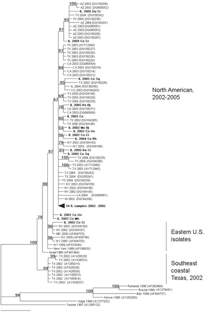
studies, large datasets of sequences are analyzed using Bayesian approaches in order to identify the most correct topology and to infer the evolutionary relationship among viral strains, considering a range of geographical scale. Bayesian approaches allowed to highlight that WNV in the USA is a geographically panmictic viral population that is nevertheless evolving and diversifying at a rate comparable to that of other positive sense RNA viral pathogens, and according to a pattern of drift and purifying selection characteristic of other arboviruses (Bertolotti et al. (2007)). Regardless of the under-lying mechanisms, our results clearly demonstrate that WNV varies genetically over geographic and temporal scales that are finer than has previously been appreciated. Our study also demonstrates that fine-scale variation in habitat characteristics within an ur-ban setting contributes to the generation and maintenance of viral diversity (Bertolotti et al. (2008); Amore et al. (in press)).

In more complex analyses, Bayesian statistics are used to provide inferences on the evolutionary rates and origins of individuals.

Indeed, recent studies used Bayesian tools in order to investigate viral geographical origins and viral dispersal patterns, describing how Bayesian phylogeography compares with previous parsimony analysis in the investigation of the H5N1 influenza A origin and epidemiological linkage among sampling localities (Lemey et al. (2009); Fusaro et al. (2010)).

In this kind of analyses, trees are hard to interpret, because of the large number of included sequences. Moreover, trees are often misinterpreted, with meaning mistakenly ascribed to the vertical proximity of taxa or clades. In cases where the vertical ordering of taxa on phylogenetic trees is flexible, the opportunity exists to ascribe biological meaning to this dimension (Maddison (1989)). In order to make unresolved trees more informative, we recently proposed the use of Evolutionary Algorithms (EAs) to find the best graphical tree representation that includes vertical information (Cerutti et al. (2010b,a)). EAs (Eiben and Smith (2003); Tettamanzi and Tomassini (2001)) are a broad class of heuristic optimisation algorithms, inspired by those biological processes that allow populations of organisms (tentative solutions of the problem to be optimized) to adapt to their surrounding environment (the problem itself): genetic inheritance and survival of the fittest. The heuristic procedure is used to find. trees that group samples with similar features in the vertical direction, and it generates at each time step a new tentative solution by rotating internal nodes. Sample order was searched in order to minimize relative distances according to their genetic distances, but this approach

(7)

Figure 2 – Phylogenetic tree constructed by Bayesian analysis of 132 WNV envelope gene se-quences. Reprinted from Virology, Volume 360, Issue 1, Luigi Bertolotti Uriel Kitron and Tony L. Goldberg, Diversity and evolution of West Nile virus in Illinois and the United States, 2002-2005, Pages 143-149, Copyright 2007, with permission from Elsevier.

could be implemented using distance matrices created from other taxon features, such as temporal or geographical data.

(8)

be necessary in order to obtain needed information on pathogens, such as their genetic and evolutionary features, as well as their distribution and diffusion.

REFERENCES

G. AMORE, L. BERTOLOTTI, G. L. HAMER, U. D. KITRON, E. D. WALKER, M. O. RUIZ, J. D. BRAWN, T. L. GOLDBERG(in press). Multi-year evolutionary dynamics of west nile virus in suburban chicago, usa, 2005-2007. Philosophical Transactions of the Royal Society B.

G. BARNARD, T. BAYES(1958). Studies in the history of probability and statistics: Ix. thomas bayes’s essay towards solving a problem in the doctrine of chances. Biometrika, 45, no. 3, pp. 293–315. L. BERTOLOTTI, U. KITRON, T. L. GOLDBERG(2007). Diversity and evolution of west nile

virus in illinois and the united states, 2002-2005. Virology, 360, no. 1, pp. 143–149. URL

http://dx.doi.org/10.1016/j.v irol .200 6.10. 030.

L. BERTOLOTTI, U. D. KITRON, E. D. WALKER, M. O. RUIZ, J. D. BRAWN, S. R. LOSS, G. L. HAMER, T. L. GOLDBERG(2008). Fine-scale genetic variation and evolution of west nile virus in a transmission "hot spot" in suburban chicago, usa. Virology, 374, no. 2, pp. 381–389. URL

http://dx.doi.org/10.1016/j.v irol .200 7.12. 040.

G. CARPI, L. BERTOLOTTI, E. PECCHIOLI, F. CAGNACCI, A. RIZZOLI(2009). Anaplasma phagocytophilum groel gene heterogeneity in ixodes ricinus larvae feeding on roe deer in northeastern italy. Vector Borne Zoonotic Dis, 9, no. 2, pp. 179–184. URL

http://dx.doi.org/10.1089/vbz .200 8.00 68.

F. CERUTTI, L. BERTOLOTTI, T. L. GOLDBERG, M. GIACOBINI(2010a). Adding vertical mean-ing to phylogenetic trees by artificial evolution. In Advances in Artificial Life: 10th European Conference, ECAL 2009. Budapest, Hungary. In press.

F. CERUTTI, L. BERTOLOTTI, T. L. GOLDBERG, M. GIACOBINI(2010b). Investigating popu-lational evolutionary algorithms to add vertical meaning in phylogenetic trees. In 8th European Conference on Evolutionary Computation, Machine Learning and Data Mining in Bioinformat-ics. Istanbul, Turkey.

A. EIBEN, J. SMITH(2003). Introduction to evolutionary computing. Springer Verlag.

J. FELSENSTEIN(1973). Maximum likelihood and minimum-steps methods for estimating evolu-tionary trees from data on discrete characters. Systematic Zoology, pp. 240–249.

(9)

J. FELSENSTEIN(1981). Evolutionary trees from dna sequences: a maximum likelihood approach. Journal of molecular evolution, 17, no. 6, pp. 368–376.

J. FELSENSTEIN(2004). Inferring phytogenies. Sinauer Associates, Sunderland, Massachusetts. R. FISHER(1912). On an absolute criterion for fitting frequency curves. Messengers of Mathematic,

41, pp. 155–160.

A. FUSARO, M. NELSON, T. JOANNIS, L. BERTOLOTTI, I. MONNE, A. SALVIATO, O. OLAL

-EYE, I. SHITTU, L. SULAIMAN, L. LOMBIN, et al. (2010). Evolutionary dynamics of multiple sublineages of h5n1 influenza viruses in nigeria, 2006-2008. Journal of Virolog, 84, no. 7, pp. 3239–47.

C. GEYER(1992). In Computing Science and Statistics: Proceedings of the 23rd Symposium on the Interface. Keramidas, EM, Ed.

G. GONNET, S. BENNER, S. ZURICH(1996). Probabilistic ancestral sequences and multiple align-ments. In Algorithm theory: SWAT’96: 5th Scandinavian Workshop on Algorithm Theory, Reyk-javík, Iceland, July 3-5, 1996: proceedings. Springer, p. 380.

P. GREEN(1995). Reversible jump markov chain monte carlo computation and bayesian model determination. Biometrika, 82, no. 4, p. 711.

E. GREGO, L. BERTOLOTTI, S. PELETTO, G. AMORE, L. TOMASSONE, A. MANNELLI(2007). Borrelia lusitaniae ospa gene heterogeneity in mediterranean basin area. Journal of Molecular Evolution, 65, no. 5, pp. 512–518.

W. HASTINGS(1970). Monte carlo sampling methods using markov chains and their applications. Biometrika, , no. 57, pp. 97–109.

P. LEMEY, A. RAMBAUT, A. DRUMMOND, M. SUCHARD(2009). Bayesian phylogeography finds its roots. PLoS Computational Biology, 5, no. 9.

W. MADDISON(1989). Reconstructing character evolution on polytomous cladograms. Cladistics, 5, pp. 365–377.

N. METROPOLIS, A. ROSENBLUTH, M. ROSENBLUTH, A. TELLER, E. TELLER, et al. (1953). Equation of state calculations by fast computing machines. The journal of chemical physics, 21, no. 6, p. 1087.

M. PRICE(1763). An essay towards solving a problem in the doctrine of chances. by the late rev. mr. bayes, frs communicated by mr. price, in a letter to john canton, amfrs. Philosophical Transactions (1683-1775), 53, pp. 370–418.

A. TETTAMANZI, M. TOMASSINI(2001). Soft computing: integrating evolutionary, neural, and fuzzy systems. Springer Verlag.

(10)