INDICE
1 INTRODUZIONE... 3
2 STRUTTURA DELL’ESERCIZIO E DESCRIZIONE DELLE FASI ... 3
2.1 FASE 1: SVILUPPO DELLA NNFL... 4
2.2 FASE 2: SCENARIO - INTERCETTAZIONE DI CAMPIONI RADIOATTIVI, VERIFICA DELLA CONSISTENZA RECIPROCA E VERIFICA DELLA CONSISTENZA CON LA NNFL ... 4
3 “MODUS OPERANDI” DEL GRUPPO DI LAVORO ENEA. ... 4
3.1 FASE 1-SVILUPPO DELLA NNFL ... 6
3.2 FASE 1-RISULTATI ... 10
3.3 FASE 2-SCENARIO: INTERCETTAZIONE DI CAMPIONI RADIOATTIVI, VERIFICA DELLA CONSISTENZA RECIPROCA E VERIFICA DELLA COSISTENZA CON LA NNFL ... 10
3.4 FASE 2-RISULTATI ... 12
4 SOLUZIONE DELL’ESERCIZIO... 12
4.1 FASE1 ... 13
4.2 FASE 2 ... 13
5 CONFRONTO TRA LE SOLUZIONI ... 13
5.1 FASE 1. ... 13
5.2 FASE 2. ... 13
6 CONCLUSIONI ... 14
7 ALLEGATO A: DETTAGLI STATISTICI FASE 1. ... 15
8 ALLEGATO B: SUMMARY REPORT ON GSV3 – PHASE 1 ... 17
9 ALLEGATO C: GALAXY SERPENT V3 – SUMMARY REPORT – PHASE 2 ... 36
1 INTRODUZIONE
Il “GALAXY SERPENT” è un insieme di esercizi internazionali virtuali web-based, focalizzati sullo sviluppo di librerie forensi nucleari nazionali (NNFL’s).
Il primo esercizio “GALAXY SERPENT exercise v.1” ha avuto luogo nel 2013 ed è consistito nella verifica della consistenza di un ipotetico combustibile nucleare esausto confiscato, con i dati nella NNFL sviluppata da ciascun partecipante.
Il secondo esercizio, il “GALAXY SERPENT exercise v.2”, è stato dedicato alle sorgenti radioattive sigillate ed è stato organizzato e gestito con la creazione di un portale dedicato, il “Central Desktop”, attraverso il quale sono state fornite tutte le informazioni necessarie. L’esercizio v.2 ha avuto inizio il 27 luglio 2015 con l’inserimento, sul “Central Desktop”, dei documenti di riferimento e dei dati (injects) necessari e sufficienti per affrontare l’esercizio stesso e ha avuto termine con la pubblicazione della soluzione in data 18 Febbraio 2016 [ADPFISS-LP1-082] (documento ANL-DHS-2016-007).
Il terzo esercizio, il “GALAXY SERPENT exercise v.3” è stato dedicato a materiali radioattivi di origine geologica contenenti Uranio (Uranium Ore Conentrate, UOC) ed è stato organizzato e gestito con la creazione di uno spazio dedicato sul portale Slack, attraverso il quale sono state fornite tutte le informazioni necessarie. L’esercizio v.3 ha avuto inizio in data 1 giugno 2017 con l’inserimento, sul portale Slack, dei documenti di riferimento e dei dati necessari e sufficienti per affrontare l’esercizio stesso e ha avuto termine con la pubblicazione, in data 13 giugno 2018, del “Galaxy-Serpent Phase 2 Summary Report”. La partecipazione di ENEA a questo esercizio è importante poiché s’inserisce all’interno delle attività già da tempo programmate e realizzate nell’ambito della sicurezza e della mitigazione del rischio chimico, biologico, radiologico, nucleare ed informatico (CBRNe). L’esercizio, pertanto, ha avuto il duplice scopo di testare da un lato il livello di competenze e il tipo di strumenti necessari a una riposta in ambito CBRN, e dall’altro di predisporre strumenti e procedure che possono vedere interessati anche altri attori a livello nazionale, in particolare nella risposta al rischio radiologico. Gli autori del rapporto, hanno portato a termine l’esercizio, contribuendo alla sua risoluzione grazie alle diverse competenze in fisica, chimica e ingegneria.
2 STRUTTURA DELL’ESERCIZIO E DESCRIZIONE DELLE FASI L’esercizio v.3 è stato strutturato in due fasi.
La Fase 1 è stata caratterizzata da uno scenario virtuale incentrato sullo sviluppo di una NNFL dedicata alle sorgenti radioattive di origine geologica (Concentrato d’Uranio, UOC), a partire dal database fornito. Gli autori dell’esercizio hanno diffuso, attraverso il portale “Slack”, un file con la descrizione del primo scenario e un file con gli 821 campioni atti a costituire la NNFL. La Fase 2 è stata concepita per verificare l’efficacia e l’utilizzo della libreria sviluppata in un contesto semplificato di analisi forense simulata. Essa è consistita in uno scenario virtuale incentrato sulla intercettazione di alcuni campioni di materiale geologico radioattivo e ha avuto, quale obiettivo, la verifica dell’eventuale corrispondenza tra i campioni radioattivi intercettati e i campioni radioattivi costituenti la libreria creata nella prima fase. Gli autori dell’esercizio hanno inserito, sul portale “Slack”, un file con la descrizione del secondo scenario e un file con la specificazione dei tre campioni intercettati.
Le informazioni generali per la strutturazione della NNFL sono state estratte dai seguenti documenti:
• “IAEA NSS2 Nuclear Forensic Support Technical Guidance Reference Manual”;
• “Proposed Framework for National Nuclear Forensic Libraries and International Directories”, J. F. Wacker (Pacific Northwest National Laboratory), U.S. Department of Energy, Michael Curry (U. S. Department of State) – 08 June 2011;
• “IAEA NSSXX DEVELOPMENT OF A NATIONAL NUCLEAR FORENSICS LIBRARY”, DRAFT, February 2013.
2.1 Fase 1: sviluppo della NNFL
La Fase 1 ha descritto una attività di importazione di concentrato d’Uranio da uno stato fittizio, Pacifica. Il governo richiede l’organizzazione delle informazioni riguardanti i materiali importati, in una Libreria Forense Nucleare Nazionale (NNFL), al fine di supportare eventuali indagini investigative forensi.
2.2 Fase 2: scenario - intercettazione di campioni radioattivi, verifica della consistenza reciproca e verifica della consistenza con la NNFL
La Fase 2 ha descritto uno scenario d’intercettazione, in seguito ad anonimo suggerimento, di un veicolo che sta cercando di lasciare il paese con un carico illecito. Individuati a bordo tre contenitori sigillati e marcati unicamente con simboli di allerta-radioattività. Le ispezioni condotte rivelano la presenza di sorgenti geologiche in ciascun contenitore e le successive indagini isotopiche specificano la presenza di concentrato d’Uranio. Il governo richiede quanto segue:
1. Verificare la reciproca consistenza dei campioni intercettati.
2. Verificare la consistenza tra i campioni intercettati e i campioni costituenti la NNFL stessa.
3. Indicare le azioni da intraprendere dopo aver risposto ai precedenti quesiti. 4. Indicare il modo di condividere i risultati all’interno del governo stesso. 3 “MODUS OPERANDI” DEL GRUPPO DI LAVORO ENEA.
Il Gruppo di Lavoro ENEA che ha partecipato all’esercizio è stato scelto sulla base delle diverse competenze (fisica, chimica, ingegneria) e sull’esperienza in campo radiologico e di campionamento ambientale. I ricercatori partecipanti sono tutti coinvolti nelle attività di security, safety e mitigazione del rischio CBRNe, della “Divisione Sicurezza e Sostenibilità del Nucleare” del “Dipartimento Fusione e Tecnologie per la Sicurezza Nucleare”.
La scelta operativa per le attività dell’esercizio ha previsto che ciascun ricercatore, singolarmente, studiasse il materiale proposto nelle tre singole fasi e, per ogni fase, è stata organizzato un incontro collegiale per lo scambio di commenti ed osservazioni.
Gli obiettivi realizzativi di tali incontri collegiali per ciascuna fase sono stati i seguenti: Ø Fase 1:
• Progettazione di un database dedicato alla raccolta dei dati relativi ai materiali radioattivi forniti dall’esercizio
• Scelta della piattaforma informatica da utilizzare per il database (sono state proposti Excel, Access, FileMaker). La piattaforma prescelta è stata Excel per la buona conoscenza di tale strumento da parte di tutti i componenti del gruppo
e per la facilità di scambio dei relativi documenti prodotti. In questa fase la scelta dello strumento, con cui progettare l’archivio, è stata guidata in maniera predominante dalla necessità di uno scambio d’informazioni pratico e funzionale e dalla comune conoscenza della struttura del database. L’esigenza di una piattaforma comune, ben nota a tutti, è fondamentale nel caso reale di una situazione di emergenza in cui, verosimilmente, si troverebbero a lavorare insieme esperti con diverse competenze e livelli di istruzione informatica. • Scelta dei parametri interrogabili da inserire nel database (cioè filtrabili) e
scelta delle informazioni che non necessitavano interrogazione (es. dati chimico fisici, tempi di emivita dei radioisotopi, costanti fisiche, …) e che pertanto sono state inserite nel database come singoli fogli elettronici non interconnessi con il database interrogabile.
Ø Fase 2:
• Discussione e scelta della metodologia più idonea per interrogare la NNFL e quindi verifica della consistenza del materiale intercettato con i campioni costituenti la libreria stessa. Questa è stata la fase più critica e complessa, in quanto si sono dovute integrare le diverse competenze, sensibilità e esperienze dei ricercatori coinvolti, cercando di focalizzarsi sulla strategia più obiettiva. È stato interessante notare come gli approcci utilizzati siano effettivamente legati, non solo alle competenze acquisite, ma anche alle esperienze lavorative degli esperti coinvolti, per cui è importante che questi tipi di esercizi prevedano anche delle attività sperimentali dedicate. La II fase è stata caratterizzata da frequenti confronti per verificare la correttezza del metodo applicato
Durante la Fase 2, la strategia scelta per il completamento delle determinazioni analitiche è consistita nell’affidare ad un singolo ricercatore l’esecuzione delle stesse e poi confrontarsi periodicamente per verificare i risultati. Tale scelta ha permesso, da un lato, di avere un esperto completamente dedicato al trattamento analitico dei dati garantendo quindi omogeneità e congruenza delle valutazioni, dall’altro di minimizzare gli errori sistematici e casuali attraverso la verifica indipendente degli altri esperti.
Nelle due fasi menzionate, la valutazione e la scelta delle strategie di interrogazione del database, invece, è stata guidata dal confronto e l’integrazione di tutte le osservazioni degli esperti, senza che ci fosse un esperto “guida” scelto a priori. Tale strategia ha permesso di verificare l’importanza dell’integrazione delle competenze e di assicurare la maggiore obiettività possibile nella risposta all’esercizio.
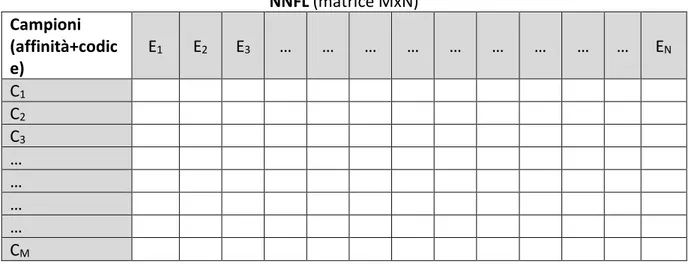
La NNFL può essere assimilata a una matrice MxN, in cui le M righe identificano gli M campioni attraverso un codice alfanumerico identificativo e la classe di affinità mentre le N colonne sono costituite dagli elementi che costituiscono i campioni e da informazioni di localizzazione; in tal modo ogni campione costituisce un punto nello spazio N-dimensionale degli elementi (Figura 1):
NNFL (matrice MxN) Campioni (affinità+codic e) E1 E2 E3 … … … EN C1 C2 C3 … … … … CM
Tabella 1: schema di principio della matrice NNFL.
3.1 Fase 1 - Sviluppo della NNFL
Il Gruppo di Lavoro ENEA ha dunque acquisito le informazioni, diffuse dagli autori dell’esercizio internazionale attraverso il portale dedicato “Slack”, per la costituzione (Fase 1) della “Libreria Forense Nucleare Nazionale” (NNFL) e per affrontare le successive fasi dell’esercizio.
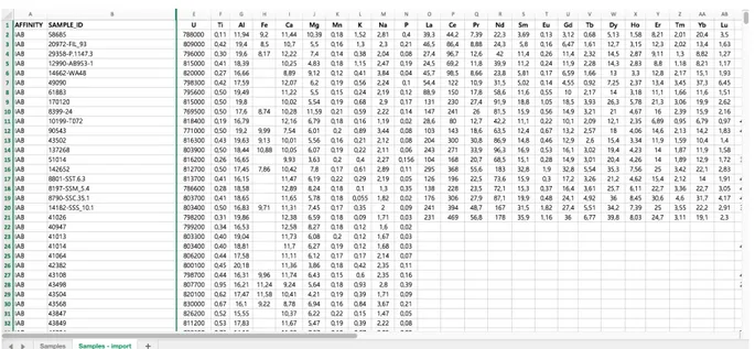
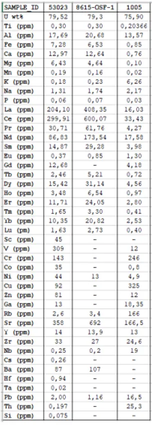
La matrice della NNFL è stata sviluppata creando un file Microsoft Excel, ordinando i campioni secondo le quattro classi di affinità previste ossia i quattro tipi di basalto (IAB, MORB, OIB, ZCRFB) da cui è stato estratto il Concentrato d’Uranio e ordinando gli elementi secondo il numero atomico. Ciascuna classe di affinità comprendeva alcune centinaia di campioni e per ciascun campione sono state riportate le seguenti informazioni:
- codice alfanumerico identificativo - latitudine e longitudine
- composizione elementale (nessuna specificazione isotopica)
La matrice della NNFL è dunque costituita da 821 righe e 49 colonne e cioè 45 colonne delle composizioni elementali più quattro colonne con le informazioni di localizzazione, classi di affinità e codici alfanumerici (Figura 2). Per le successive analisi, si è ritenuto di poter trascurare le colonne riportanti le informazioni di localizzazione e pertanto la matrice della NNFL è risultata costituita da 821 righe e 47 colonne. Presenti, dunque, 821 campioni e 45 elementi con concentrazioni espresse in ppm, tranne che per l’Uranio i cui valori sono stati espressi in wt%. Per uniformare le unità di misura si è proceduto a convertire la concentrazione dell’Uranio in ppm.
Tabella 2: estratto dalla matrice NNFL (Fase 1).
Ognuno degli 821 campioni della libreria è rappresentabile da un punto in uno spazio a 45 dimensioni oppure, in altri termini, i 45 elementi definiscono uno spazio a 45 dimensioni popolato da 821 punti. Si è in presenza di un tipico problema multivariato definito da 45 variabili eventualmente correlate. Si è reso pertanto necessario ricorrere ad un approccio per gestire efficacemente un tale insieme di dati e cioè un approccio che consenta di trarre informazioni che spieghino e diano ragione dei dati stessi. L’approccio per gestire i dati contenuti nella matrice della NNFL è stato basato sull’utilizzo di una tecnica statistica avanzata, l’Analisi delle Componenti Principali (ACP), eseguita per mezzo di MATLAB v. R2014a.
La ACP appartiene alle tecniche statistiche di analisi multivariata, ed è applicabile a insiemi di osservazioni iniziali eseguite al fine di disporre di un vasto ambito di informazioni, conseguenti a indagini condotte su campioni più o meno vasti. L’obiettivo dell’ACP consiste nell'individuare alcuni (pochi) fattori di fondo che spieghino e diano ragione dei dati stessi. Tali fattori di fondo, o componenti, rappresentano delle dimensioni “ideali” dotate di significato. La ACP realizza la possibilità di esprimere in forma sintetica insiemi di variabili tra loro correlate riducendo il numero delle variabili stesse. Si tratta, cioè, di ricombinare le misure individuando strutture lineari indipendenti che possano essere interpretate come indici non correlati.
I dettagli della ACP sono riportati in Appendice A.
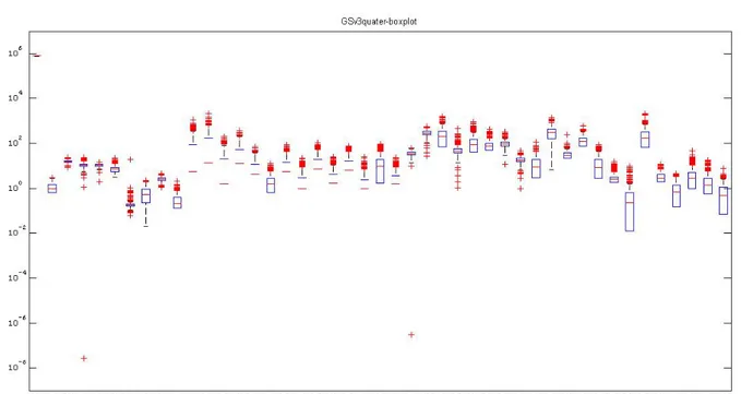
Dalla matrice è stato eliminato l’Uranio per i seguenti motivi:
• Esso spiega circa il 95% della varianza conducendo così ad un risultato fortemente condizionato
• Esso presenta la minore variabilità rispetto a tutti gli altri elementi (vedi figura 3) • Esso non è un “trace element”
• Esso è il principale componente dei campioni della NNFL e pertanto non è utile ai fini di una investigazione di tracciabilità
Figura 1: box-plot con la variabilità dei 45 elementi del database.
Di conseguenza, il numero delle colonne degli elementi è stato ridotto da 45 a 44 e così la ACP è stata portata a termine sulla matrice 821x44. Tale matrice presentava tuttavia dei dati mancanti e pertanto, prima della escuzione della ACP, essi sono stati ricostruiti per mezzo di stime fisicamente neutre ottenute applicando l’algoritmo di MATLAB, Alternate Least Square (ALS). La successiva esecuzione della ACP ha mostrato che le prime cinque componenti spiegano circa il 95% della varianza, le prime tre componenti pricipali spiegano circa il 83% della varianza e le prime due componenti principali spiegano più dei due terzi della varianza ossia circa il 71% (vedi figure 4 e 5).
Figura 2: grafico a barre (screeplot) con la precentuale di varianza spiegata dalle prime cinque componenti principali.
E’ stato pertanto ragionevole considerare le prime tre componenti principali in modo da ridurre le dimensioni dello spazio da 44 a 3 oppure anche le prime due componenti principali in modo da ridurre le dimensioni dello spazio da 44 a 2.
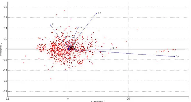
L’interpretazione dei risultati è stata resa possibile rappresentando in un unico grafico “bi-plot“, gli 821 campioni e le 44 variabili. Il grafico bi-plot consente di visualizzare congiuntamente i coefficienti delle prime componenti principali ortonormali per ciascuna delle 44 variabili e i coefficienti delle prime componenti principali ortonormali (scores) per ciascuna delle 821 osservazioni (campioni).
Ciascuna delle 44 variabili è rappresentata da un vettore le cui direzione e lunghezza quantificano il contributo della variabile alle componenti principali che costituiscono il nuovo sistema di riferimento [Figura 3].
3.2 Fase 1 - Risultati
La prima componente principale (asse orizzontale) mostra, per quanto visibili con il fattore di ingrandimento impostato, coefficienti positivi per gran parte delle variabili e cioè per Bario, Stronzio, Cerio, Lantanio, Neodimio (e altri) e coefficienti negativi per Cromo e Nichel (e altri). La seconda componente principale (asse verticale) mostra, per quanto visibili con il fattore di ingrandimento impostato, coefficienti positivi per Cerio, Stronzio, Lantanio, Cromo, Nichel, Neodimio (e altri) e coefficienti negativi per il Bario (e altri).
E pertanto, è stato possibile affermare che:
§ I maggiori coefficienti per la prima componente principale corrispondono agli elementi Ba, Sr, Ce, La.
§ La seconda componente principale consente di distinguere tra campioni caratterizzati da elevati valori di concentrazione di Ce, Sr, La, Cr, Ni, Nd (e altri) e campioni caratterizzati da piccoli valori di concentrazione di Ba (e altri).
3.3 Fase 2 - Scenario: intercettazione di campioni radioattivi, verifica della consistenza reciproca e verifica della cosistenza con la NNFL
Il Gruppo di Lavoro ENEA ha acquisito le informazioni, diffuse dagli autori dell’esercizio internazionale attraverso il portale dedicato “Slack”, relative ai tre campioni intercettati.
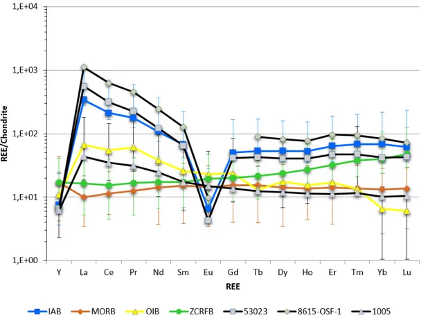
La valutazione della consistenza fra i tre campioni ignoti e fra i campioni ignoti e la NNFL, è stata portata a termine utilizzando un metodo basato sugli schemi delle Terre Rare (REE) come principali indicatori per l’appartenenza alle delle classi di affinità.
L’utilizzo dei “trace elements”, come riportati nel database originario, è stato giustificabile poichè la variazione della loro concentrazione è connessa con la geochimica delle rocce e con le formazioni geologiche e fenomeni di degradazione in modo che essi possano essere utilizzati per valutare l’origine delle rocce e dei processi (naturali o antropogenici) che hanno subito. Inoltre, una variazione significativa della loro concentrazione, confrontata con le concentrazioni attese (in matrici simili), potrebbe essere rappresentativa dei processi di produzione. L’utilizzo dei “trace elements” è dunque importante per affrontare il problema dell’origine di campioni sconosciuti. In particolare, anche il gruppo delle “Terre Rare” (REE) può essere utilizzato per verificare l’origine dei campioni e dei processi che hanno subito, con particolare riferimento ai processi tecnologici e alle applicazioni tecnologiche.
Gli schemi delle REE sono stati costruiti utilizzando i loro valori normalizzati rispetto alla condrite carbonacea (secondo il database “Taylor & McLennan, 1985), escludendo lo Scandio a causa della sua assenza in due dei tre campioni intercettati.
Nella [Figura 4], gli schemi delle Terre Rare dei tre campioni intercettati (53023, 8615-OSF-1,
1005)sono confrontati con i medesimi schemi della NNFL, per ogni tipo di basalto. Le barre d’errore rappresentano l’intervallo min-max per ciascun valore delle REE.
Figura 4: schemi delle REE dei tre campioni intercettati (punti in grigio), confrontati con gli schemi REE della NNFL (normalizzazione dal database “Taylor & McLennan”, 1985).
3.4 Fase 2 - Risultati
Osservando la [Figura 4] è stato possibile rispondere ai primi due quesiti previsti per la Fase 2:
§ Gli schemi REE dei primi due campioni intercettati (53023, 8615-OSF-1) si adattano bene agli schemi REE della classe di affinità del basalto IAB.
§ Lo schema REE del terzo campione intercettato (1005) mostra un comportamento più ambiguo; esso, infatti, si adatta bene alla classe di affinità del basalto OIB fino all’Europio mentre dal Gadolinio al Lutezio sembra adattarsi meglio alla curva del basalto MORB.
L’inconsistenza reciproca fra i tre campioni intercettati rende più complesso lo scenario del traffico illecito suggerendo la possibilità di una infrazione multipla della catena di controllo dei materiali.
Riguardo al terzo quesito previsto per la Fase 2, sono state individuate, in un contesto prettamente scientifico/tecnico, le seguenti azioni principali:
§ Condurre analisi radiologiche e chimiche sui pneumatici e sedili del veicolo intercettato e anche sugli indumenta degli individui a bordo.
§ Selezionare un gruppo specializzato di esperti con abilità geologiche per investigare più approfonditamente le proprietà dei materiali intercettati.
§ Condurre ulteriori analisi chimiche e test morfologici sui campioni intercettati per la deduzione delle origini geografiche e per rilevare qualsiasi indizio di processamento tecnologico implementato.
§ Predisporre ispezioni nelle miniere di Uranio per controllare l’inventario e le licenze. Si ritiene, inoltre, che, in un contesto di carattere investigativo, potrebbero risultare utili anche le azioni di seguito riportate:
§ Allertare la IAEA e i paesi limitrofi.
§ Ricostruire i movimenti del veicolo con il carico illecito.
§ Fermare e controllare altri veicoli che appartengano alla stessa azienda di trasporti cui appartiene il veicolo intercettato.
§ Incrementare i controlli ai confini attraversati dal veicolo con il carico illecito.
Riguardo al quarto quesito previsto per la Fase 2, al fine di condividere le informazioni tra le istituzioni governative, si potrebbe redigere un dettagliato rapporto tecnico confidenziale che sia distribuito alle competenti autorità pianificando riunioni di coordinamento dedicate a gruppi specializzati.
4 SOLUZIONE DELL’ESERCIZIO
Gli autori dell’esercizio hanno prodotto un rapporto per la Fase 1 e un rapporto per la Fase2, proponendo la propria soluzione per i primi due quesiti della Fase 2.
4.1 Fase1
Il rapporto prodotto dagli autori per la Fase 1 è un sommario delle risposte di tutti i gruppi che hanno partecipato all’esercizio.
Il rapporto è riportato in Appendice B. 4.2 Fase 2
Il rapporto prodotto dagli autori per la Fase 2 è un sommario delle risposte di tutti i gruppi che hanno partecipato all’esercizio e comprende la soluzione proposta dagli autori stessi riguardo ai quesiti 1 e 2.
Il rapporto è riportato in Appendice C. 5 Confronto tra le soluzioni
Si riporta di seguito il confronto tra le soluzioni. 5.1 Fase 1.
Sia gli autori dell’esercizio, sia il Gruppo di Lavoro ENEA hanno scelto di utilizzare un comune foglio di calcolo Microsoft Excel per realizzare la libreria. Tale scelta è in sintonia con la necessità di una veloce consultazione da parte di esperti con diverse competenze informatiche e di uno scambio di informazioni efficace, per cui l’utilizzo di un programma ben noto alla maggior parte degli esperti è condiviso da entrambi gli approcci. Tale scelta, d’altra parte, presenta alcune limitazioni in termini di funzionalità aggiuntive, rispetto ad altri programmi di archiviazioni più specifici, o laddove ci sia una numerosità e complessità superiore di informazioni riguardanti le sorgenti. Rimane in ogni caso fondamentale l’approfondimento della necessità di interscambio delle informazioni e di protezione dei dati sensibili.
5.2 Fase 2.
Il Gruppo di Lavoro ENEA, confrontando gli schemi REE del database e dei campioni intercettati, è giunto ai seguenti risultati:
1. I primi due campioni intercettati “53023” e “8615-OSF-1” si adattano bene agli schemi REE della classe di affinità del basalto IAB e sono pertanto reciprocamente consistenti. 2. Lo schema REE del terzo campione intercettato “1005” mostra un comportamento più ambiguo; esso, infatti, oltre a non essere consistente con gli altri due campioni intercettati, si adatta bene alla classe di affinità del basalto OIB fino all’Europio mentre dal Gadolinio al Lutezio sembra adattarsi meglio alla curva del basalto MORB [Figura 4].
Gli autori dell’esercizio hanno riportato i seguenti risultati:
1. I campioni “53023” e “8615-OSF-1” sono reciprocamente consistenti ed è identificata l’affinità IAB nel modello della NNFL.
2. Il campione “1005” è risultato non consistente con gli altri due campioni o con nessuna delle quattro classi di affinità rappresentate nel modello della NNFL.
6 CONCLUSIONI
Dal confronto tra le soluzioni per la Fase 2 si evince quanto segue:
1. La soluzione degli autori è stata coerente con la soluzione del Gruppo di Lavoro ENEA (GLE): i campioni intercettati “53023” e “8615-OSF-1” risultano recirocamente consistenti ed entrambi consistenti con la classe di affinità IAB del modello della NNFL. 2. La soluzione degli autori è stata parzialmente coerente con la soluzione trovata dal Gruppo di Lavoro ENEA. Entrambi i gruppi hanno concordato sulla non-consistenza del campione “1005” con gli altri due. Riguardo alla consistenza del campione “1005” con le classi di affinità del modello della NNFL, il GLE ha letto lo schema REE attribuendo al campione un adattamento parziale e simultaneo alle REE delle classi di affinità IOB e MORB. Gli autori hanno invece affermato la non-consistenza del campione in oggetto con alcuna delle classi di affinità.
Gli autori non hanno fornito indicazioni sul metodo utilizzato per ottenere i propri risultati e pertanto la divergenza di cui al punto 2 potrebbe essere considerata meramente interpretativa anziché sostanziale.
7 ALLEGATO A: dettagli statistici Fase 1.
Descrizione sintetica della tecnica statistica “Analisi delle Componenti Principali” (ACP). [7] [8] La formulazione più nota della ACP è attualmente quella proposta da Hotelling nel 1933 e si basa sull’ipotesi che i valori di un insieme di p variabili originarie correlate siano determinati da un più ristretto insieme di variabili mutuamente indipendenti. Tali variabili vengono determinate come combinazione lineare delle variabili originarie in modo tale da massimizzare il loro successivo contributo alla varianza totale dell’insieme. Il sitema delle osservazioni è organizzato in forma matriciale, costruendo una matrice pxq (righe x colonne), con q osservazioni e p variabili (mutuamente dipendenti ossia correlate). Le q osservazioni sono rappresentabili da punti in uno spazio p-dimensionale (spazio delle righe).
Obiettivo della ACP è ridurre la dimensionalità dello spazio delle righe, in modo da rappresentare la variabilità del problema utilizzando un minor numero di fattori, ossia utilizzando il minor numero di dimensioni possibile (dimensionalità intrinseca del problema). Si tratta, dunque, di costruire un sottospazio m-dimensionale (m<p) i cui assi coordinati (le componenti principali) si allineino con l’insieme dei dati originari.
Le p variabili correlate originarie, costituiscono una variabile multivariata rappresentata da un vettore in uno spazio p-dimensionale. Per tale variabile multivariata è possibile definire una funzione densità di probabilita (FDP) multivariata, con i propri parametri di localizzazione e dispersione e cioè un vettore valor medio e una matrice di covarianza. Quest’ultima quantifica l’ampiezza della FDP definendo il grado di correlazione tra le p variabili originarie ed è una matrice non-diagonale.
La ACP consente di diagonalizzare la matrice di covarianza, per mezzo di una opportuna variazione del sistema di riferimento (rotazione), ottenendo così un nuovo insieme di variabili ortogonali mutuamente indipendenti e di conseguenza la FDP multivariata è esprimibile come una semplice produttoria di FDP univariate. In tal modo le nuove variabili (Componenti Principali) sono combinazioni lineari delle variabili originarie e poiché la matrice di covarianza nella base delle Componenti Principali è diagonale, la varianza totale è la somma delle singole varianze delle Componenti Principali.
In sostanza, lo scopo della ACP è la rappresentazione di un insieme di dati in uno spazio p-dimensionale, con matrice di covarianza non-diagonale, in un sottospazio m-dimensionale (m<p) con matrice di covarianza diagonale. La ACP è classificata come metodo del secondo ordine poiché la riduzione della dimensionalità dello spazio è basata unicamente sulle proprietà della matrice di covarianza (momento del secondo ordine).
La prima Componente Principale, ossia il primo asse del nuovo sistema di riferimento nel sottospazio m-dimensionale, è calcolata in modo tale da descrivere una quantità di varianza originaria maggiore della varianza associata a ciascuna singola variabile. In altri termini la prima Componente Principale è la direzione in cui si realizza la massima dispersione dei dati (criterio su cui si basa la formulazione di Hotelling) e quindi essa spiega la massima percentuale della varianza dei dati, in una dimensione.
Calcolando la seconda Componente Principale si otterrà la direzione ortogonale in cui si realizza la massima dispersione dei dati, ma inferiore alla precedente, e pertanto le due componenti principali spiegheranno la massima percentuale della varianza originaria in due dimensioni. E così via, le componenti principali successive spiegheranno una sempre minor percentuale della varianza originaria, nel sottospazio m-dimensionale. La conoscenza della
percentuale di varianza spiegata è essenziale per l’interpretazione dei grafici delle componenti principali.
In estrema sintesi formale si ha che, date p variabili osservate X, si costruiscono p combinazioni lineari Y del tipo:
Y
1= a
11X
1+ a
12X
2+ … + a
1iX
i+ … + a
1pX
p…
Y
k= a
k1X
1+ a
k2X
2+ … + a
kiX
i+ … + a
kpX
p…
Y
p= a
p1X
1+ a
p2X
2+ … + a
piX
i+ … + a
ppX
pLe combinazioni lineari Y, nomate “Componenti Principali”, devono soddisfare le seguenti condizioni:
1. Assenza di correlazione:
Cov(Y
k’, Y
k) = 0, ∀ k’ ≠ k
2. Ordine in relazione alla quantità di varianza complessiva che ciascuna variabile può sintetizzare:
V(Y
1) ≥ V(Y
2) ≥ … ≥ V(Y
i) ≥ … ≥ V(Y
p)
3. La varianza complessiva dei due sistemi di riferimento deve coincidere: " 𝑉$𝑌&' = " 𝑉(𝑋+)
-+./
-&./
Il sistema delle Xi variabili originarie è ridondante essendo esse correlate. Di conseguenza, per riassumere adeguatamente i dati, sarà sufficiente considerare solo le prime m (m<p) componenti principali, ammesso che queste forniscano un adeguato contenuto informativo. Il criterio più immediato per la scelta del numero m di componenti rispetto a cui rappresentare il fenomeno presuppone che venga prefissata la proporzione della variabilità complessiva che si desidera tali componenti spieghino, ad esempio i due terzi oppure il 70/80%; m sarà perciò il minor numero di componenti per le quali tale percentuale è superata.
8 ALLEGATO B: Summary Report on GSv3 – Phase 1
Galaxy Serpent
Version 3 (GSv3)
Summary report on Galaxy Serpent version 3 – Phase 1
Contents
• Explanatory Notes………..…..…Page 18 • Summary of Responses to Question 1……….………Page 19 • Summary of Responses to Question 2………….………Page 20 • Summary of Responses to Question 3……….………Page 21 • Summary of Responses to Question 4……….………Page 22 • Summary of Responses to Question 5……….……Page 23 • Sampling of Submitted Figures……….…………Page 26 • Acronyms Used………Page 35
Explanatory Notes
The following report is a summary of responses from teams submitting Phase 1 reports for the Galaxy Serpent – version 3 exercise. 29 teams comprising 132 individuals participated in the GSv3 exercise. 22 of these 29 teams (76%) submitted Phase 1 reports as of December 15, 2017. Responses provided by teams are summarized by question prompt below. Results cited reflect the work of teams answering a given question. Not all reports addressed each question, and multiple tools (Excel, R, etc.) or statistical methodologies were utilized by teams, thus the numbers cited do not necessarily sum to the number of reports submitted. Some teams also submitted free-form reports rather than responding question-by-question, and on occasion reports did not address questions directly – in such cases best inferences or judgements were made. Individual quotes, graphs, or results are given without attribution to maintain anonymity, and serve to illustrate some of the various approaches and methodologies teams employed.
Acronyms used are identified on the final page of this document. About 8 of the 22 respondents included plots or graphs in their reports. Some of these are included near the end of this report. They were not selected on the basis of efficacy or to suggest more frequent use by teams, but rather to present a representative sample of different techniques that teams reported utilizing in organizing the data and looking for discriminating signatures. This document is not intended as an “answer key” or set of “how-to” instructions, nor to convey how the exercise organizers “expected” teams to proceed through Phase 1. Rather, its purpose is simply to report the techniques various teams applied in terms of approaches and methodologies in organizing the provided data, which sometimes led to different preferred analytical paths. For example, some teams viewed trace elements as the main discriminator (largely due to gaps in data provided for REEs), while others addressed the missing REE data and viewed them as the main determinant.
The Galaxy Serpent exercise organizers would again like to thank all teams and individual participants for their dedication and involvement, and to acknowledge the devoted effort by all. We recognize that this work is conducted in addition to your normal duties, and deeply appreciate the commitment and effort both in this exercise, and in maturing the discipline of nuclear forensics, of all those involved.
Summary of Responses to Question 1
1) Prompt: How did you organize the data? Did you use all of the signatures provided? If not, which ones did you use or not use, and why?
There was no universal approach employed by teams when organizing the data but many common themes emerged. A variety of valid methods were used, with many teams combining multiple approaches. Teams generally ignored the latitude/longitude fields as they were unrelated for material discrimination, and some retained the sample ID while others did not.
All teams kept the “affinity” or “class” descriptor (OIB, MORB, IAB, or ZCRFB), with many making separate worksheets for each. Teams employed a variety of techniques to categorize the data, ranging from elementary to more complex in nature, and looked for elemental groupings providing distinctive signatures. Teams generally combined machine learning approaches, using algorithms that can learn from data without relying on rules-based programming, with statistical or latent variables approaches, looking for discerning relationships among given or processed data. Reports varied in the level of specificity regarding the methods employed, but a couple teams stated that they used box plots and/or histograms to investigate which elements and/or groupings of elements might prove useful for distinguishing affinities. A couple teams reported using histograms to combine REE data (especially Eu, Tb, Yb, Lu) with Ti, Zr, Hf, Nb, Ta (group IV and V) data; and combining group IV transition element Zr, Hf, Ti data with alkaline-earth/group IIA elements (Ca, Sr, Ba) and Pb data.
All teams seem to have separated data by affinity, and most additionally divided data along the lines of trace elements and REEs. For REEs, some teams used both provided data and “normalized to chondrite” values, while the majority discussed using only the normalized values. One team reported challenges in finding all normalization factors. Another found the “analysis of REE normalized pattern is a very powerful technique for the identification of UOC origin,” and another also decided to “focus on lanthanides in the dataset, as they are a good indicator of UOC-origin.” One team noted their decision to use REEs (after chondrite normalization) and additional key elements like Ti, Mn, K, Th, Zr, or elemental correlations such as Ca/Sr, Na/K. Most teams did not go into this level of specificity in their reports, but many seemed to have come to thematically similar conclusions.
At least one team assessed data based on discerning geologic ratios (eg. La/Sm vs Zr; Nb/Y vs Zr). One team described separating data using classifications of small vs large ionic radii elements and REEs (received, and chondrite normalized), which were analyzed to evaluate diagnostic properties, and key correlations and covariances.
The primary difference in how teams organized data centered on how they handled the missing data. About 5 teams explicitly discussed the possible approaches they saw in this this regard, noting that one could i) replace missing data by mean or median values, which could affect reliability; ii) use dummy variables to fill gaps, which some noted may not be the best option for a large numerical dataset; or iii) delete the deficient data, which may
be adverse for multivariate statistics as it can artificially reduce data. Among teams who specifically noted their approach in this regard:
• Three teams chose to ignore elemental data that was over 30% deficient. o One of these teams noted that for this reason they did not use Fe, Sc, Co, Cu,
Zn, Ga, Nb, Sn, Cs, Hf, Ta, Pb, Th, Si, l, Sn, or the lanthanides due to effect missing data would have on reliability
• One team noted excluding Fe, Sn, Ga due to the sparse nature of data
• One team reported they considered all elemental data, but excluded those with missing values on a case-by-case basis by considering the effect of these missing values
• Two teams opted to exclude U as, one team stated, “it explains 95% of the variance (a very biased result)” and because “it is a main component (not a trace element), and thus not useful in a traceability investigation”
• Six teams opted to use “all signatures” Summary of Responses to Question 2
2) Prompt: Which technical approaches did you use to evaluate and interrogate the provided UOC data? (For example, statistical regression, principal component analysis, comparative/correlative assessments, etc.)
Teams varied in the degree of detail given in outlining the technical approaches they employed. A few teams used fundamental Excel analysis as their primary tool, while the majority of teams used Excel as a precursor to discern discriminatory patterns and/or prepare given or processed datasets for more complex analysis. Teams using Excel noted looking at ranges, histograms, box plots and the like. Two teams noted using ANOVA and descriptive statistics prior to additional analysis.
Techniques teams reported using for further analysis included both latent variable and machine learning approaches, with most teams using multiple methods in combination. Due to the varying degrees of specificity in discussing the specific methods used by teams, it was sometimes challenging to clearly characterize the methodologies used. With this stipulation, it appears that, of the 22 teams submitting reports:
• Fifteen teams used PCA
• Four teams using PCA did so in conjunction with PLS-DA, “a machine learning algorithm that attempts to explain variance through latent variables while
simultaneously dividing data into classes, with imputation being used to fill in the dataset due to the large amount of missing data”
• Four team reported using PCA in conjunction with OPLS-DA
• Four teams reported using “statistical/multivariate analysis methodologies” including cluster analysis with PCA; LDA for outlier testing and comparative assessment; and MVA based on a self-developed algorithm
• Two teams used “discriminant analysis”
• Four teams reported using classification/decision trees, random forest ensembles, and neural networks for comparative assessments of impurity distributions, ratios and chondrite-normalized REE patterns
• Three teams reported using “statistical regression” • One team noted using “hierarchical cluster analysis” • One team noted using “pattern analysis”
• One team reported using REE data for a “consistency check” for each affinity, looking for outliers, calculating relative differences, and plotting selected data • One team reported using “comparative and correlative methods”
• Two teams noted using “comparative assessments using elemental ratios” by normalizing all data to standard chondrite values, and then plotting the normalized concentrations by increasing atomic number
• One team reported using “subjective and variational-statistical estimation of data, as well as graphical visualization of data sets”
PCA was by far the most commonly named technical approach, being cited explicitly by at least 15 of the 22 teams submitting Phase 1 reports. Teams generally applied PCA using trace element concentrations to observe data clustering. Some teams reported poor discrimination for PCA applied to REEs due to missing data, while other teams who replaced missing data (see page 3) reported being able to reduce dimensionality. One such team noted they found the first three principal components explained 85% of variance, allowing them to reduce dimensionality to 3. Another team reported using PCA as “unguided learning technique to look for groups/patterns in data” coupled with discriminant analysis to improve the discrimination ability between perceived groups. Teams analyzing REE data reported a series of possible paths, sometimes used in conjunction, including i) before normalization without replacing missing data; ii) after chondrite normalization without replacing missing data; iii) before normalization replacing missing data using geometric means/medians; and iv) after chondrite normalization replacing missing data using geometric means/medians. One team reported determining geometric means using an ALS algorithm.
Summary of Responses to Question 3
3) Prompt: Did you use a commercial software package to evaluate and interrogate the data? If so, which one? (For example, Excel, R, Sigma, etc.)
Most, but not all, teams utilized Microsoft Excel, many citing its availability and convenience since the data was provided as .xls files. While not always explicitly state it appears that, of the 22 respondents, roughly:
• 4 (~18%) used only Excel
• 15 (~68%) used Excel in concert with other software packages • 3 (~14%) did not utilize Excel in any significant way
The majority of teams seem to have used some combination of free (R, Simca-P, etc.) and commercial (Matlab, Origin, etc.) software packages. Of the teams using Excel in combination with other software packages, Excel was often utilized for some lower-level tasks (data preparation, initial data evaluation, preliminary analysis and comparison, REE
normalization, etc.) while additional software packages were used for more complex analyses. Teams reported using the following non-Excel software packages:
• R; a free package (6 teams)
o One team additionally used Shiny (R package for interactive web application)
o Teams used R in statistical analysis environment for PCA, LDA decision trees and/or randomForest analyses
• Matlab; a commercial package (4 teams)
o For MVA, PCA, and/or developing homemade algorithms) • Origin/OriginPro; a commercial package (3 teams)
o For histograms, boxplots, ANOVA, PCA • Simca-P; a free package (2 teams)
• SPSS Statistics; a commercial package (1 team) • Anaconda; a free package (1 team)
o Used with Orange, a data mining add-on • PAST; a free package (2 teams)
• JMP; a commercial package (1 team)
• Solo from Eigenvector Research; a commercial package (1 team) • Python; a free package (1 team)
o Planned use for future (post-exercise) analysis of provided data Summary of Responses to Question 4
4) Prompt: What was your approach if you did not use commercial software? Did you develop your own tool, or did you take a different approach? (For example, subject matter expert-driven)
The 22 responding teams interpreted this question in a variety of ways. 12 explicitly noted the essential role that SMEs played in driving the analysis, while 10 cited no other “tools” being used. However, in the latter group SME-driven analysis clearly played a vital and necessary role in working through Phase 1 of the exercise. Those explicitly citing the role of SMEs used their proficiency in the following reported ways:
• SME-driven approach to signature selection, data analysis and interpretation
(including REE interpretation and pattern analysis); drawing of confidence intervals (7 teams)
• SME developed indigenous code (5 teams)
o For use in Phase 2 to help relate unknown material data to specific samples from the model NF database (1 team)
o For developing an MVA original computation tool for material discrimination analysis use with NF in Phase 2 to help compare unknown material data to specific samples from Phase 1 database (1 team)
o For developing a homemade specific statistical tool (3 teams)
• Several teams alluded to the vital role SMEs play, but noted that this would not be fully leveraged until the Phase 2 analysis
Summary: While not explicitly mentioned in the responses, all teams clearly used a SME-driven approach (whether in statistics, geochemistry, nuclear forensics, etc.) to data analysis and interpretation, with several teams alluding to the critical role this will play in Phase 2. Teams also leveraged SMEs in developing indigenous code for handling and analyzing the data.
Summary of Responses to Question 5
5) Prompt: What features of the provided data were the most useful?
The vast majority of respondents did not address this lead-in question, instead placing their responses in the sub-questions below. For those that did respond:
• One team reported trace elements/impurities were the most useful data
• One team reported that no single variable was “most useful,” but the fact that all four classes contained enough information to give distinct patterns was of the greatest discriminatory benefit
• One team reported the process of interrogating data graphically with histograms and box plots comparing data for the four affinities led to their conclusion that REE and select trace element concentrations were the most useful.
a. Prompt: Did you utilize isotopics? Why or why not?
All teams noted that uranium isotopic concentrations were not provided, thus isotopics were not used. Several teams used ratios of various provided elemental concentrations as a discriminating signature. Some teams added that some useful isotopic ratios that could be key NF signatures, if isotopic concentrations had been provided, would be (234U/238U), (235U/238U), and Sr (87Sr/86Sr), and Pb (208Pb/204Pb) ratios. Some teams also noted that the 234U/230Th ratio can be used to calculate UOC age assuming all Th was removed from the sample during cleaning, and that any loss or addition of Th (228Th/232Th) could also be used as an isotope chronometer.
b. Prompt: Did you utilize trace elements? Why or why not?
All teams used trace element concentrations with the exception of one which reported that the missing data limited reliability as a classification/identification tool, but thought they might be useful when comparing to an unknown in Phase 2.
Several of the teams using trace elements reported that they “are one of the most significant signatures for the material discrimination analysis.” About 10 teams specifically noted their providing a “useful signature for clues about processing history and geolocation” as well as the potential manufacturer. In discussing the potential for origin assessment, several teams explicitly noted that trace elements can “indicate special technological processes (added chemicals or contaminants) which can identify/exclude producers.”
In terms of specific analytical methods, many reiterated that they used both trace element and REE signatures in combination. Additionally, teams noted the usefulness of the following techniques in considering trace elements:
• Three teams noting organizing trace elements for each affinity into five levels based on concentration, and some teams stated they constituted the main useful data signatures in their analyses
• One team noted using box plots and histograms to assess all trace element data, and then focusing further analysis to a select few trace elements based on their variance
• One team cited observed correlations between trace elements for different affinities
• One team noted examining trace element data, but not finding it very useful at this point
• One team discussed limited success in using trace elements arising from challenges in finding normalization factors for some elements, and there being missing data for others, finding that elements (Ba, Ta, and Nb) and a plot of normalized concentration ratios of Ba/Nb vs Ta/Nb appeared distinctly unique across the four different affinities and could aid as a significant signature Also, as noted earlier in the Question #2 discussion:
• Several teams again mentioned PCA as a valuable technique
• One team mentioned machine learning techniques using SME knowledge • One team noted they split the data into three groups based on i) REEs, and ii)
small and iii) large atomic radii to help identify the most diagnostically valuable elements and groupings
c. Prompt: Did you utilize rare earth elements? Why or why not?
All teams responding reported using REE data which many teams stated had strong discriminating power as seen by the differences in their mean concentrations across the four affinities. Many teams wrestled with the question of whether the high discriminating power of the REEs was overshadowed by the large amounts of missing data. For example, one team concluded that only Sc and Y had enough data to be included when considered along with trace elements but may have some value when comparing groups to “unknowns,” while another team decided only the lanthanides had enough data to be useful as an identifier regarding composition and potential origin.
Teams utilized REE data in multiple analyses. Several commented that there were fairly clear differences in REEs among the affinities, and several noted the particularly “marked Eu dip” in the IAB data which was not present for the other affinities. A couple teams stated that the lack of data for these elements mitigated their usefulness. One team succinctly summarized: “This raises the question: Is consistency within an affinity significant if there is only 6% of REE data present for any one affinity (OIB)?”
• Eight teams explicitly noted that REE signatures can also characterize local geochemical mineralogical conditions and features at the uranium mining site, and that samples of UOC from different places of origin will likely have individual
REE-signatures which can be linked to ore genesis and the geological origin and technological processing of the sample.
o In addition to noting that REEs constituted a very powerful technique for identifying UOC origin, one team noted that SEM images and XRD data would have been very useful attributive data for UOC characterization o One team noted REE patterns are useful in determining geographical
origin, but due to the sparsity of data used them as an auxiliary determinant
• Six teams discussed challenges in using REEs due to the sparsity of the data: o Due to the large amount of missing REE data, one team built a separate
and smaller model which was “solely based on REEs with 112 samples (included any sample with at least one of 14 REEs included)”
o One team normalized, and removed samples without REE data giving “useful dimensionality reduction”
o One team went into some detail on the question of the impact of the significant amount of missing REE data, noting that “the influence of the REEs may be questionable.” This team made PCA scatter bi-plots (one of which is included for illustration in the figures) which conveyed the “discriminating power of the elements by their length and direction.” They noted that since “the majority of the REE point in a very similar direction..[t]his suggests that they all behave similarly when subjected to PCA analysis and therefore having data for all of the REEs may not be necessarily valuable for this method. Eu however points in the opposite direction to the other REE and may be more useful for PCA than the other REEs. The poor separation achieved…is likely attributed to the absence of the more discriminating REEs.”
• One team stated they used the REEs, but with limited success given their challenges with the randomly missing data, and in finding normalization factors for some elements. As referenced earlier, this same team found certain elements (Ba, Ta, and Nb) and derived plots of normalized concentration ratios of Ba/Nb vs Ta/Nb, appear “distinctly unique against the four different affinities and can aid as a significant signature”
• About 8 teams commented on aspects of the missing REE data as it related to effectively applying PCA.
o One team used box plots and histograms of all REEs, a comparison of
normalized REE data, and PCA to show that REEs were useful in distinguishing between affinities
o One team reported using REEs by plotting chondrite normalized
concentrations, and applying PCA. Based on population differences between classes, they developed a short list of trace elements for further PCA
investigation, excluding others with data missing from further consideration in their analysis
o One team noted that, “despite being sparsest dataset, REEs remain
clearly defined clusters, and use of the chondrite-normalized REE patterns provides comparative distinction between the four affinities”
• One team noted that the analysis of chondrite-normalized REE content made it possible to separate the samples from the deposits. Also, analysis of graphs of the ratio of elements, such as Yb/Eu or Lu/Zr, made it possible to “practically guarantee that the sample belongs to one of four deposits,” and thus serve as a valuable discriminator
• One team used REEs in latent variables approaches utilizing SME knowledge Sampling of Submitted Figures 1
1*As noted in the introductory overview, about 8 of the 22 respondents included plots or graphs in their reports.
Some of these are included near the end of this report. They were not selected on the basis of efficacy or to suggest more frequent use by teams, but rather to present a representative sample of different techniques that teams reported utilizing in organizing the data and looking for discriminating signatures.
Acronyms Used
• ALS = Alternative Least Square • ANOVA = Analysis of variance
• JMP = no acronym, a statistics package offered by Statistical Analysis System (SAS) • LDA = linear discriminant analysis
• NF = nuclear forensics • MVA = multivariate analysis
• OPLS-DA = Orthogonal Projection to Latent Structures Discriminant Analysis • PAST = Paleontological Statistics software package
• PCA = principal component analysis
• PLS-DA = Partial least squares discriminant analysis • REE = Rare earth element
• SME = Subject matter expert
• SPSS = Statistical Package for the Social Sciences • UOC =uranium ore concentrate
9 ALLEGATO C: Galaxy Serpent v3 – Summary Report – Phase 2
In Phase 1 of the Galaxy Serpent exercise teams were asked to organize provided surrogate UOC data into a model National Nuclear Forensics Library (NNFL) for the purpose of responding to questions posed by authorities in the course of an investigation involving nuclear or other radioactive (RN) material. The data was derived and repurposed from open-domain geological deep sea core surveys for basaltic core samples. Such data, with the SiO2 concentration relabeled as uranium and after some statistical manipulation, closely mimics uranium ore concentrate (UOC). By design, the data set was sparse and featured missing elements in order to mirror characteristics of actual UOC data sets and to pose decisions and challenges to participants. Teams responded to prompts regarding the methodologies they used, and their efficacy, in leveraging distinguishing characteristics to discriminate between the four classes of samples represented in the data (IAB = Island Arc Basalt; MORB = Mid-Ocean Ridge Basalt; OIB = Mid-Ocean Island Basalt; ZCRFB = Columbia River Flood Basalts). Phase 1 responses were submitted by 23 of the 29 participating teams (79%); this was reported without attribution in the Phase 1 summary report.
In Phase 2, teams were presented with a hypothetical scenario in which three barrels of UOC were found out of regulatory control. Teams were asked to respond to the following queries from authorities about its potential common provenance and consistency to holdings in the model NNFL developed in Phase 1:
1. Based on a comparison of material characteristics, does the UOC in each of the barrels share a consistent provenance with either of the other two barrels? Describe the methodologies or techniques by which you reached this conclusion.
2. Is any of the UOC consistent with the material you recorded in your NNFL during Phase 1? Be specific in reporting whether each individual sample (coded 53023; 8615-OSF-1; 1005) was consistent with your library. Describe the methodologies or techniques by which you reached this conclusion, particularly as it relates to the interrogation of the library created in Phase 1. 3. What steps would you, or your government, take after determining the answers to the previous two questions? How would you share the results internally within your own government? What confidence do you have in your reported results, and how did you arrive at this (qualitative or quantitative) confidence level?
Phase 2 responses were submitted by 22 of the 29 participating teams (76%). Responses to the first two prompts were, in general, more detailed than those for the third prompt. An unattributed summary of the responses from teams is given below in Table 1. The findings that exercise organizers anticipated is given in the first row in bold: Specifically, a) unknowns “53023” and “8615-OSF-1” are consistent with each other, and b) identified with the IAB affinity in the model NNFL; and c) unknown “1005” was not consistent with the other two unknowns, or d) with any of the four affinities represented in the model NNFL. All responding teams (22 of 22) came to the same findings on questions a), b) and c). However, some teams (5 of 22) came to a different conclusion on d), finding that unknown “1005” was consistent with one or more of the four affinities in the model NNFL as summarized below. Details on the methods used to reach these findings follow the table.
Discussion of Responses to Prompt 1
Prompt 1 asked: Based on a comparison of material characteristics, does the UOC in each of the barrels share a consistent provenance with either of the other two barrels? Describe the methodologies or techniques by which you reached this conclusion.
All teams submitting reports (22 out of 22) found that unknowns 53023 and 8615-OSF-1 shared a common provenance, and that unknown 1005 was not consistent with either unknown 53023 or 8615-OSF-1.
Several teams additionally noted that while unknowns 53023 and 8615-OSF-1 shared a consistent provenance, they were not from the same sample; that is, their provenance was consistent, but not identical.
The details and specificity of the reports varied. Some teams provided summary findings with minimal discussion of how they reached their conclusions, while others provided greater detail as to their methodologies and underlying thought processes.
Missing data
A handful of the reporting teams (~3-5) made some reference to the missing data within the unknowns 8615-OSF-1 and 1005. Two teams discussed this in some detail; one noting three options they considered:
1. Deleting or ignoring the data which they viewed as problematic as it cuts too much of data set)
2. Inserting dummy variables, with they reasoned was not the best option with a large dataset 3. Replacing the missing data with mean or median value of the set. They chose this option for the GSv3 exercise, but noted it can be inaccurate if missing data is not missing completely at random (MCAR) which could be the case here as large blocks of lanthanide data were missing. This affected the confidence of their findings.
Several (2-4) teams appear to have used option 3, as inferred from plots; only two mentioned this directly.
Rare Earth Element (REE) data
Most (19 of 22) teams explicitly noted the use of REE data in their analysis, and others may have done so as well, but not noted this overtly in their report. The main reason some did not utilize REE data seems to be the missing data in unknowns 8615-OSF-1 and 1005. About ten of the teams noted that REE data was the “main discriminant fingerprint,” and provided valuable information as to both origin and history.
Teams found that chondrite normalized REE patterns for unknowns 53023 and 8615-OSF-1 showed significant similarity in pattern, although the REE concentration for unknown 53023 was about a factor of two lower than unknown 8615-OSF-1. Team determined that unknown 1005 was markedly different from the other two unknowns, and thus was not of consistent provenance. Most teams made explicit reference to the Eu anomaly in this regard.
Several teams also cited REE data comparison in their conclusion that while unknowns 53023 and 8615-OSF-1 are of consistent provenance, they are not from the same sample. As evidence, they noted that the normalized values of REE of 8615-OSF-1 sample were approximately twice that of sample 53023, the missing Gd content for unknown 8615-OSF-1, and the variation in the Sr and Ni content between the two.
A couple teams noted that in addition to normalizing to standard chondrite values, normalizing to Tb, a marker of uranium ore deposition, provided further confirmation of their conclusions.
Elemental concentrations: 13 of 22 teams explicitly noted the use of non-REE impurity data in their analysis, all in conjunction with REE analysis. Roughly six teams noted challenges associated with the absence of any measurement uncertainties. (The announced exercise guidance was that measurement uncertainties were not provided since variation within class was assumed to be much greater than any analytical uncertainty.)
Many teams noted the uranium concentration of unknowns 53023 and 8615-OSF-1 were similar, while unknown 1005 was slightly lower.
Relative Standard Deviation (RSD) analysis:
Three teams employed a coefficient of variation analysis as a way to determine if different pairing of two of the three sets of data suggested consistent provenance. The standard deviation of each element represented in the library dataset was calculated. Averages of the four RSDs were then used to compare the relative differences between pairing of unknowns. Scores were assigned, ignoring missing data. For example, one team awarded results within one-RSD three points, results within two-RSDs two points, results within three-RSDs one point, and results greater than three-RSDs no points. These results were then tallied for each pairing of unknowns. The results of such an approach are given below.
Discussion of Responses to Prompt 2
Prompt 2 asked: Is any of the UOC consistent with the material you recorded in your NNFL during Phase 1? Be specific in reporting whether each individual sample (coded 53023; 8615-OSF-1; 1005) was consistent with your library. Describe the methodologies or techniques by which you reached this conclusion, particularly as it relates to the interrogation of the library created in Phase 1.
The responses to this prompt were the most varied in terms of findings and in reports did not always elucidate the methods used to reach conclusions.
Teams used a variety of methods in interrogating the data for the unknowns, and conducting a comparative analysis with affinities represented in their model NNFL. The results are summarized in Table 5 on the following page. In addition to the methods previously noted, a few teams additionally employed box plots, LDA, Random Forest, and other techniques. Table 5 represents a method-by-method summary of findings. “No” means teams did not find that method as suggesting a given unknown was of consistent provenance with a given affinity; “Possible” means a method found the unknown was possibly consistent with an affinity based on that method alone; and “Yes” indicates a method found the unknown was consistent with an affinity. Numbers in parenthesis indicated the number of teams reaching this finding. Where there are no numbers, all teams reported the finding. Some reports did not provide sufficient detail to make a determination. In general, teams that identified unknown 1005 as being consistent with an affinity in the model NNFL appear to have utilized one comparative method. In a handful of cases, it was difficult to determine whether a team was reporting a provenance match as a confident finding, or a suggested possible finding worthy of further examination. In such cases “best possible inferences” were made.
While all teams determined that unknown 53023 and 8615-OSF-1 were consistent with the IAB affinity with a high degree of confidence, the majority noted that the finding was less strong for unknown 8615-OSF-1.
Only three teams made mention that unknown 8615-OSF-1 exactly matched a specific IAB sample identification in the model library. Those that compared these directly reported that the elemental concentrations were consistent, with the exception of Sr, but not identical.
Rare Earth Element (REE) data
Rare earth elemental comparison appears to have been used by the majority, if not all, of reporting teams. The Eu anomaly and slope across all elements exhibited by unknowns 53023 and 8615-OSF-1 was also present in affinity IAB. None of the other affinities displayed the Eu anomaly. Teams cited this as the primary evidence in concluding that 53023 and 8615-OSF-1 share a common provenance with affinity IAB. Many noted that this conclusion was stronger with 53023 than with 8615-OSF-1 due to slight differences in Y concentrations, and the missing Gd signature. Many found the third unknown, 1005, shared no similarity in terms of specific features or slope to any other affinity, leading most teams to conclude it was extremely unlikely to share a common provenance with any known affinity in the model NNFL. However, some teams noted that the REE pattern of 1005 bore some similarity to OIB for
the lighter REEs, and to MORB for the heavier REEs, leading them to include these as a potential common provenance.
Sample plots for this section are shown below.
Non-REE concentration comparison
Results here were similar to REE concentration comparative analysis, but the reported findings were more consistent across teams. Teams found that 53023 and 8615-OSF-1 were of consistent provenance as affinity IAB, with stronger confidence for 53023 than with 8615-OSF-1 due to slight differences in K, Ni, Nb, Sr and Zr concentrations. In general, unknown 8615-OSF-1005 was not found to be consistent with any affinity by this method.
PCA - REE
Unknowns 53023 and 8615-OSF-1 were found to be nearest the IAB affinity by this method. Both fell within the known IAB sample points, while teams found that 53023 was consistently closer to the center of the IAB cluster than unknown 8615-OSF-1, giving relatively higher confidence. Most teams found that unknown 1005 did not lie within the most distant scattered points for any affinity in the model NNFL, however about five teams determined that unknown 1005 lay within the OIB, MORB or ZCRFB clusters, suggesting that, by this method, it was possible that 1005 was consistent with those affinities. One team suggested this consistency was sufficient to report a consistent provenance with affinity OIB.
PCA on non-REEs
Teams using this method generally found that unknowns 53023 and 8615-OSF-1 were of consistent provenance as the IAB affinity, and unknown 1005 did was not consistent with any of the four affinities. A few groups found possible correlations of unknowns with certain affinities, as summarized in the table above.