UNIVERSIT `
A DEGLI STUDI DI PISA
Facolt`a di Ingegneria
Corso di Laurea in Ingegneria Aerospaziale
Tesi di Laurea
A Code for Surface Modeling and Grid
Generation Coupled to a Panel Method for
Aerodynamic Configuration Design
Relatori:
Prof. Aldo Frediani
Dott.Ing. Giovanni Bernardini
Laureando:
An integrated platform has been developed which features a geometric, a grid gen-eration and an aerodynamic analysis module. The main intent is to execute a quick though reliable preliminary aerodynamic analysis on a generic complex aerodynamic configuration and, at the same time, provide a mean of exporting the defined geom-etry or grid to leading CAE/CAD, meshing and analysis softwares, for deep detail modifications or more accurate, although time consuming, analysis.
In the geometric module, the process of shape definition is easily and intuitively achieved with the aid of specific features and tools. The geometric description relies on NURBS, a flexible, accurate and efficient parametric form. Once the configu-ration has been defined, the user is ready to move on the grid geneconfigu-ration module, or to export it to IGES standard format in order to use CAE/CAD, meshing or aerodynamic analysis programs.
The grid generation module is capable to build structured or unstructured meshes. Both of the processes are automatized, even if the user can easily set and control grid parameters. The structured grid generator is oriented to LaWGS description standard, while the unstructured grid can be exported to different formats.
The user is now ready to launch Pan Air, a panel method, as the aerodynam-ic solver. The preprocessor and postprocessor aid to the definition of the flow parameters and to the graphical visualization of the results.
One of the strength of this code is the user friendly GUI organization of each module: the user is aided throughout all the steps. Besides this, every module relies
on fast computational algorithms to speed up the overall process.
For all these reasons, this code has a natural lean to be used in pair with an optimization tool.
Alla fine di questo lungo percorso, `e giusto fermarsi un momento e guardarsi intorno, ma soprattutto indietro ed un dovuto e sentito pensiero va a chi mi `e stato vicino, a chi mi ha aiutato ed a chi a contribuito in modo importante al raggiungimento di questo traguardo.
Volendo percorrere la strada a ritroso, la prima persona alla quale va un caloroso ringraziamento `e il Professor Aldo Frediani, in lui ho trovato entusiasmo, coinvol-gimento ed ha riacceso in me una passione per lo studio negli ultimi anni un po’ affievolitasi.
Ringrazio anche il mio correlatore Giovanni Bernardini, per l’umanit`a dimostra-ta e il tempo e la pazienza che mi ha dedicato, ma cosa ancora pi`u impordimostra-tante lo ringrazio infinitamente per il grande bagaglio di conoscenze che `e riuscito a trasmet-termi.
Non posso certo dimenticare la Professoressa Maria Vittoria Salvetti che tra una battuta e l’altra mi ha sempre sostenuto, dimostrando di credere nelle mie capacit`a, anche se spesso volubili.
Spostandomi in ambito ludico un ruolo determinante in questi anni lo hannno ricoperto i miei migliori amici, che hanno contribuito a preservarmi dal logorio dello studio, facendomi cos`ı arrivare fresco, ma un po’ in ritardo, a questo appuntamento! Sicuramente un ringraziamento speciale va alla mia dolce met`a Giulia che senza lasciarsi scoraggiare dal mio carattere impossibile mi `e stata vicina negli ultimi due anni, aiutandomi in maniera decisiva e donandomi la stabilit`a e la serenit`a di cui
avevo bisogno per affrontare questo percorso.
Il ringraziamento finale va alla mia famiglia, alla quale non sono mai riuscito ad esprimere direttamente la mia gratitudine, ma alla quale spero di aver regalato in questa giornata grande gioia e soddisfazione.
Summary I
Acknowledgements III
Introduction 1
1 ASD: Aerodynamic Shape Design 5
1.1 Introduction . . . 5
1.2 ASD Surface Generator . . . 6
1.2.1 The Main Window . . . 6
1.2.2 The Features and the Feature Windows . . . 6
1.2.3 The Body Feature . . . 6
1.2.4 The Wing Feature . . . 9
1.2.5 The Bulk Feature . . . 15
1.2.6 The Wingbody Feature . . . 16
1.2.7 The Inlet/Outlet Feature . . . 18
1.2.8 The Fillet Feature . . . 23
1.2.9 The Tfillet Feature . . . 27
1.2.10 The Wround Feature . . . 29
1.2.11 Viewing the Results . . . 30
1.3 ASD Surface Mesher . . . 33
1.4.1 Airfoil Manager . . . 37
1.4.2 NACA Airfoil Generator . . . 39
1.4.3 Section Sketcher . . . 40
1.4.4 Flap Sketcher . . . 41
1.5 ASD Limitations . . . 45
2 NURBS (Non Uniform Rational B-Spline) 51 2.1 A Brief Historical Survey . . . 51
2.2 Curve and Surface Basics . . . 54
2.2.1 Implicit and Parametric Forms . . . 54
2.2.2 Advantages and Disadvantages . . . 55
2.2.3 Requirements for the parametric forms . . . 56
2.2.4 Power Basis Form of a curve . . . 57
2.2.5 B´ezier Curves . . . 57
2.2.6 Tensor Product Surfaces . . . 62
2.3 B-Splines . . . 65
2.3.1 Shortcoming of polynomial and B´ezier forms . . . 66
2.3.2 B-Spline Basis Functions . . . 67
2.3.3 B-Spline Curves . . . 74
2.3.4 B-Spline Surfaces . . . 81
2.4 Rational B-Splines . . . 87
2.4.1 Nurbs Curves . . . 88
2.4.2 Nurbs Surfaces . . . 91
2.5 Fundamental Geometric Algorithms . . . 92
2.5.1 Knot Insertion . . . 93
2.5.2 Knot Removal . . . 93
2.5.3 Degree Elevation . . . 95
2.5.4 Degree Reduction . . . 96
2.5.5 Other Advanced Geometric Algorithms . . . 96
3 Free Form Surface Design 97 3.1 Introduction . . . 97
3.2.2 Local Interpolation . . . 103
3.2.3 Transfinite interpolation . . . 105
3.3 Parameterization . . . 107
3.3.1 Uniform Parameterization . . . 107
3.3.2 Chord Length Parameterization . . . 108
3.3.3 Centripetal Parameterization . . . 108
3.3.4 Performance of the Different Parameterizations . . . 108
3.3.5 Knot Vector Selection . . . 109
3.3.6 Parameterization and Knot Vector Selection for Surfaces . . . 110
3.4 Notion of Continuity . . . 111
3.4.1 Continuity of Curves . . . 111
3.4.2 Continuity of Surfaces . . . 115
3.5 Visual Aspects of Continuity . . . 117
3.6 Implementation of G2 or C2 Continuity with Local and Global Algo-rithms . . . 118
3.6.1 Limitations of the Local Approach for G2 or C2 Continuity . . 118
3.6.2 Limitations of the Global Approach for C2 continuity . . . 119
3.7 Variational Analysis and Modeling of Free Forms . . . 121
3.7.1 Fairness of Curves and Surfaces . . . 121
3.7.2 Constrained Optimization . . . 123
3.7.3 Conclusions . . . 126
4 Surface Modeling in ASD 127 4.1 The old Algorithms featured in ASD . . . 127
4.1.1 ASD Curve Algorithm - local interp crv . . . 127
4.1.2 ASD Bicubic Surface Algorithm - local interp sfc . . . 132
4.2 The new Geometric Algorithms . . . 134
4.2.1 The new Curve Algorithm - global interp crv . . . 134
4.2.2 The new Surface Algorithm - global interp sfc . . . 141
4.3 The ASD Advanced NURBS GUI . . . 145
4.3.1 C1 Algorithm Parameter . . . 145
4.3.2 C2 Algorithm Parameter . . . 146
4.3.3 Lofting . . . 147
4.4 Some Results with the new Geometric Engine . . . 147
4.5 Future Improvements . . . 151
5 Structured Grid Generation Module 153 5.1 Introduction . . . 153
5.1.1 Grid Connectivity-Based Classification . . . 154
5.1.2 An Overview of Structured Mesh Generation . . . 155
5.2 The New Grid Generation Module . . . 157
5.3 Requirements for the Structured Grid Generation . . . 158
5.3.1 ASD and the Mesh . . . 158
5.3.2 Pan Air and the Mesh . . . 159
5.4 Logics and Mesh Organization . . . 160
5.4.1 Subdivision in Logical Subsets . . . 160
5.4.2 Meshing the Logical Subsets . . . 162
5.4.3 Connections between Logical Subset Grids . . . 165
5.5 The Structure Grid Generation Interface . . . 169
5.5.1 Wing and Body Feature Parameters . . . 169
5.5.2 Mesh Generation . . . 170
5.5.3 Mesh Analysis and Stats . . . 170
5.5.4 Plotting Tools . . . 170
5.5.5 Grid Storing . . . 170
5.5.6 Pan Air Preprocessor Launcher . . . 171
5.6 Examples of Structured Grid Generated . . . 171
5.7 Limitations and Future Improvements . . . 172
6 Panel Method: Pan Air 177 6.1 Panel Methods . . . 178
6.2 Pan Air . . . 189
6.2.1 Pan Air Capabilities . . . 190
6.2.2 Pan Air Technology . . . 191
6.2.3 Pan Air Geometry Input . . . 192
6.2.4 An overview of configurations analyzed with Pan Air . . . 194
7 Pan Air Pre/Post Processor Module 201 7.1 Pan Air Preprocessor . . . 201
7.2 Pan Air Postprocessor . . . 210
7.3 A simple testcase . . . 217
8 Conclusions 223
List of figures 227
A Evaluation of the stiffness matrix 235
Nowadays the preliminary design optimization holds an important role in the overall design process. To be efficient, optimization needs a high degree of automation, leaving to the designer only small and fast tasks. The efficiency would be enhanced if the different modules are part of the same environment, that is, with a unique integrated platform.
The preliminary aerodynamic property estimations represent the basis from where to start further investigations and modifications. Although theoretical prediction or lower order aerodynamic solver, like vortex lattice softwares, may be enough accurate for an early preliminary design, when investigating innovative configurations, like the
PrandtlPlane one, the order of approximation may be unacceptable, mainly because
its effect can lead to unreliable results. For example, PrandtlPlane stability is highly sensitive to small aerodynamic load variations, thus more refined analysis should be undertaken. Moreover, the gained experience with the traditional configurations in aeronautics, may not always help.
This and other related problems lead to the need of an efficient and fast code for preliminary evaluation, capable also to export the geometrical shapes to international standard formats, in order to eventually submit more accurate analysis. Since the steps for obtaining an aerodynamic analysis consist in a geometrical configuration definition, a grid generation and a program pre and postprocessing, the main idea is an integrated environment where preliminary aerodynamic design and optimization could be easily and quickly undertaken.
In the first chapter an overview of ASD capabilities and tools is given. ASD (aerodynamic shape design) is a tool written in Matlab language, for geometric shape design of aerodynamic surfaces purposes. Further, it features an internal unstructured mesher. In this chapter, the process of generating configurations is analyzed step by step, mainly from the user perspective; also the use of the tools is shown. A brief description of the integrated unstructured mesher is also given. Finally, the geometric limitations of the code are pointed out: they concern the continuity of the generated NURBS surfaces. The practical drawbacks are discussed, showing the need of a geometric engine improvement.
Second chapter deals with NURBS, a parametric form. First, a brief historical survey is given, followed by the definition of some noteworthy parametric forms, like B´ezier and B-spline, fundamental to NURBS understanding. After, NURBS are analyzed, and some important algorithm important for their manipulation and implementation are briefly discusses.
The third chapter is of main importance, since it discusses how NURBS are effectively built over a set data points. The interpolation problem is analyzed in depth, as well as parameterization problems. Then, continuity is discussed from three different perspectives; the effects of continuity on shape fairness are briefly shown. Finally, implementation of new algorithms, based on fairness and variational modeling, and overcoming the previous limitations, is carried out.
Next chapter shows more in detail the capabilities of the new algorithms compared with the old ones. The new GUI, where the interpolation parameters are controlled, is presented. The chapter ends with some pictures of configuration generated with the new algorithms.
Chapter five treats grid generation. After a short introduction on grid generation topic, and especially on the structured mesh, the requirements of the aerodynamic solver Pan Air on the input networks are pointed out. Thus, the logics adopted in the grid generation process and all its underlying reasons are discussed in depth. The parameters which control the mesh generation, and the graphical interface are finally presented, as well as some examples of networks generated.
of its capabilities, its requirements, and some of its applications are presented. The integration of Pan Air within the platform is pointed out in chapter seven. Both the preprocessor and the postprocessor are presented in details, with the aid of pictures of analyzed configurations. A final simple test case is submitted, with the aim of checking Pan Air predictions and its grid sensitivity.
1
ASD: Aerodynamic Shape Design
1.1
Introduction
ASD (Aerodynamic Shape Design) is a fully parametric, modular, scriptable aero-dynamic surface generator. One of ASD peculiarity is the easy and fast new con-figuration generation and existing concon-figuration modification capability, due to the parametric approach and the user friendly graphical interface. Another trademark is the ability to generate non-conventional configurations, such as the PrandtlPlane one, whose aerodynamic shapes can not be easily designed using conventional CAD soft-wares. Together with this geometric capabilities, ASD is provided of a meshing tool, capable of producing triangular meshes and hybrid tri-quad meshes suitable both for aerodynamic and electromagnetic simulations and featuring automatic wakeline recognition for aerodynamic panel solvers. ASD surface mesher can export various formats from panel neutral .dat files to standard .stl tri mesh. The output of the surface generator can be exported as set of trimmed NURBS into an IGES file or fed into meshing tool built into the code. Some useful tools aid the users to sketch the geometric shapes, such as the airfoil manager, the section manager, the Naca airfoil manager and the flap sketcher.
Due to its characteristics, ASD main field of application is the early stage of aerodynamic design. In this stage, in fact, ASD can quickly generate a huge number of configurations, making it possible to analyze many different layouts during the
1 – ASD: Aerodynamic Shape Design
initial optimization process.
The ASD code has been written in Matlab, and requires, a part from Matlab, the Spline Toolbox.
Whereas more details are required, refer to [1; 2; 3; 4].
1.2
ASD Surface Generator
1.2.1
The Main Window
As soon as the program interface starts, the main window (fig.1.1) is brought on focus. The main window is made up of 8 list boxes and a menu bar. The list boxes show the features currently in memory, and allow the user to remove or modify existing features or to add new ones. Double clicking on a feature opens the corresponding modify window. In every list box feature are listed showing the feature tag and ordered as they have been defined. The features that contain surface data are marked with a “ ==> ” right before the tag. Every list box allows multiple selections. The
Generate selected and Mesh selected pushbuttons pass the selected surfaces to the
surface generation function and to the meshing tool respectively. It is to be noted that only feature that contain surface data can be meshed. The View pushbutton opens the Surface Viewer.
1.2.2
The Features and the Feature Windows
It is worth a note that only body, wing and inlet/outlet features are independent, being the remaining features just connections. Each feature can be added and edited through its own window, which appears selecting the Edit voice on the menu, or just double-clicking on the feature.
1.2.3
The Body Feature
The Add/Modify Body interface enables to specify all the parameters involved in the generation of a Body feature. The interface for this feature is shown in fig. 1.2. Using these parameters, the code generates a skeleton of the body and then
Figure 1.1: The ASD main window.
interpolates it using a bi-cubic NURBS. A scheme of the skeleton along with the body lines is shown in the picture 1.3. The Tag field lets the user specify a tag for the feature which will be stored along with all the parameters and will be shown in the ASD main window list boxes. The Upper/Lower Section list box contains the list of used body sections. Using the Add and Remove pushbuttons the user can add or remove body sections selecting appropriate .dat files. Next to each list box there is the number of section files listed. The number of upper and lower sections must be equal for the surface generator to work. The fields X0, Y0, Z0 are the coordinates of the first section of the list. The coordinate system used in ASD has the positive x-axis in the direction of the fuselage, starting from the nose, the positive y-axis is directed spanwise from the fuselage toward the wing tip, while the positive z-axis is normal to both x and y and directed upward. If Y0 is set to 0 the body is assumed
1 – ASD: Aerodynamic Shape Design
Figure 1.2: The body feature window.
to be on the symmetry plane and no other action is taken, otherwise the shape is simmetrized on the plane y=Y0. The field Frame Spacing contains the x coordinates of the body sections relative to X0. The fields Body lines are used to specify the
.dat file containing body lines data. The user can both browse for the file or input
the complete path. Pressing the Preview pushbutton will plot on a separate figure a preview of the skeleton and of the resulting interpolated surface, as shown in fig. 1.4.
Figure 1.3: Parameters involved in the definition of the body feature
Figure 1.4: Preview of the skeleton and resulting interpolated surface for a body feature.
1.2.4
The Wing Feature
The Add/Modify Wing interface lets to specify all the parameters involved in the generation of a Wing feature. The interface for this feature is shown in fig.1.5. Using these parameters the ASD code generates a skeleton of the wing which is then interpolated with a linear-cubic NURBS where the linear direction is spanwise.
1 – ASD: Aerodynamic Shape Design
Figure 1.5: The wing feature window.
An example is shown in fig. 1.6. The Wing Airfoils list box contains the list of used airfoils. Using the Add and Remove pushbutton the user can add or remove airfoils selecting appropriate .dat file. The Add pushbutton opens a standard get dir dialog which defaults on the standard UUIC AIRFOIL DATABASE directory. Upon selecting a directory, the Airfoil Viewer window opens and lists all the airfoils
Figure 1.7: The Airfoil Viewer window
found in this directory (fig.1.7). The Airfoil Viewer enables the user to see origi-nal points in the file selected, re-interpolated airfoil using an arbitrary number of points. It also enables the user to calculate camber and maximum thickness of the airfoil selected. All of the plot options act only on the visualization of the airfoil
1 – ASD: Aerodynamic Shape Design
on this window. The airfoil loader function loads the original set of points, clos-es the trailing edge if found open, locatclos-es the leading edge, sets the chord parallel to the x-axis and of unitary length and re-interpolates the points using a chord-wise cosine distribution of 50 points. The same set of action is performed when the Interpolated (cosine distr. chord // x axis) radiobutton is selected (see al-so the Airfoil Generator and the Airfoil Manager sections). The popup Wing type is used to select if the wing being created is to be freely placed, or is to be connected with other wings. When the wing is free, the position and shape of the wing is derived from the information of X0, Y0, Z0, dihedron and sweep angle. If the feature is linked to another wing then the last airfoil is linked to a spanwise section of another wing. The user must thus specify which airfoil on the linking wing is to be matched, along with the ID of the linked wing. This is used to constrain a wing to follow the wing it is linked to. This feature is useful to define T-tails.
The X0, Y0, Z0 are the coordinates of the nose of the first airfoil on the list (assumed to be the root airfoil). If Y0 is set to 0 and the dihedron angles are all 90◦
or −90◦ then the wing is assumed to be on the symmetry plane, so only the upper
or lower side of the airfoil is considered.
The Ribs Spacing field contains the spanwise position of the airfoils relative to the first airfoil. The Chords field contains the chords of the airfoils listed, Lambda and Dihedron contain the sweep and the dihedron angle of the defined bays; Alpha,
Beta, Theta contain information on the rotation angle of the airfoils around the three
principal axes, x, y and z, respectively.
If the wing type is set to “linked”, then the Linked Wing ID popup menu is used to select which wing is to be linked to. Obviously there must be some wing defined to define a linked wing, as self referencing is not allowed. The Rib Link Spanwise field is used to select the spanwise section position on the wing is to be linked to. The user can make use of expressions involving other wing feature, as long as they have been already defined, which are evaluated before saving the result. For example the expression
wing(2).y0 + wing(2).ribs spacing(2)
a textbox where the result of evaluation is displayed.
Figure 1.8: The Preview wing feature
Pressing the Preview pushbutton will plot on a separate figure a preview of the skeleton and of the resulting interpolated surface, as shown in fig.1.8
Every wing feature can have a variable number of control surfaces defined. They are all listed in the Flap/Slat list box. Double-clicking on one of the listed features opens the corresponding Add/Modify Mobile Surface window (fig.1.9.
Within the aim of this window, it is possible to generate mobile surfaces on a wing, both on LE (slat) and TE (flap, aileron etc). The mobile surface must be defined within one single bay. Parameters describing the mobile surface are the ribs
spacing, to set the spanwise position, the gap, which specifies the relative gap, in
percentage of the length of the mobile surface, to leave between the mobile surface and the main wing surface, the chords, to set the chords at fist and last spanwise section.
The mobile surface sectional geometry is created by a tool called Flap Sketcher (section 1.4.4).
1 – ASD: Aerodynamic Shape Design
Figure 1.9: The Add/Modify Mobile Surface window
Figure 1.10: Mobile surface deflection
Finally, a flap/slat motion law is stored in a plain text .dat, so that when selecting a slat and flap deflection angle, the mobile surface configuration is properly achieved.
1.2.5
The Bulk Feature
Figure 1.11: The bulk feature window
The bulk feature is specifically designed to link the two wing tips of a biplane configuration as shown in fig.1.12. The bulk feature creates a connection element
Figure 1.12: A bulk example
between two wings, by smoothly transform one airfoil to the other, giving the user the ability to select the bulk start and end airfoil. The airfoil transformation is linear along the bulk midline (see fig.1.13).
1 – ASD: Aerodynamic Shape Design
Figure 1.13: The bulk control parameters
The popup menu Upper Wing and Lower Wing are used to select which wing is to be the start(end) wing. In the Bulks upper (lower) airfoil the user specify the airfoil to be used for the upper (lower) end of the bulk feature. It can be selected using the airfoil viewer. The Upper (Lower) Wing Control Line specify the vertical and horizontal distance of the linear part of the bulk feature from the wing last airfoil. Finally, the Upper(Lower) Wing Round Bay Intervals contains the number of sections that have to be created along the round from the start wing to the beginning of the linear part of the bulk. The minimum number is two. The intermediate airfoils are created linearly spacing and morphing the first airfoils to the last one on the other side of the bulk.
Pressing the Preview pushbutton will plot on a separate figure a preview of the skeleton and of the resulting interpolated surface in dark transparent gray, and the two wings that take part at the generation in light transparent gray, as shown in fig.1.14
1.2.6
The Wingbody Feature
The WingBody feature is a wing-like surface to blend to a generic root section of a wing. The result is a smoothly blended surface that extends the wing to the
Figure 1.14: The Preview Bulk figure
Figure 1.15: The wingbody feature window
section specified by the user using different options to control section smoothness and generation. As a wing-like feature, it retains several definitions and parameters typical of the Wing feature.
1 – ASD: Aerodynamic Shape Design
The Add/Modify WingBody interface (fig.1.15) enables to specify all the param-eters involved in the generation of a wingbody feature. The X0, Y0, Z0 are the coordinates of the foremost point of the root section. The editable field Root Section
Name is used to specify the .dat file containing root section data. The file should
contain an airfoil-like set of bi-dimensional coordinates, with unit chord. The chord of the root section is specified in the following field. The Beta and Dihedron editable fields contain information on the rotation angle of the airfoils around the y axis and the dihedron angle of the wingbody respectively.
The Linked to Wing and Linked Airfoil ID popup menu list all the wings currently defined and lets the user select the one to which the wingbody feature is to be linked to, and lets the user select which airfoil is the one the wingbody feature is to be linked to. Finally, the LE Fillet Type and TE Fillet Type popup menus allow the user to control the type of leading edge and trailing edge connection. The two conditions are independent and are linearly blended one into the other moving from the LE to the TE. The 3 types of connections are:
1 z-der = 0 : the derivatives at the wing interface are preserved, thus preserving the smoothness of the surface; the derivatives at the root section are the same as the wing derivatives except for the z component which is set to zero; 2 z-der = 0, x-der = 0 : the derivatives at the wing interface are preserved, thus
preserving the smoothness of the surface; the derivatives at the root section are the same as the wing derivatives except for the z and x component which are set to zero.
3 Linear: all derivatives both on the wing interface and on the root section are set equal to the vector connecting the two.
Fig. 1.16 and 1.17 clarify the connection modality.
1.2.7
The Inlet/Outlet Feature
The inlet/outlet feature is a body-like feature specifically designed to generate the cavity of an inlet or outlet. The inlet/outlet surface is built by interpolation of a set
(a) Type 1 on LE and TE. Front view (b) Type 1 on LE and TE. Top view
(c) Type 2 on LE and TE. Front view (d) Type 1 on LE and TE. Top view
Figure 1.16: WingBody creation, type 1 (a) and (b), type 2 (c) and (d).
of frames. The interface gives the user the control over the spatial position of these frames, allowing a quick and easy way to parametrically modify the surface. The generation of the inlet/outlet feature also takes care of intersecting the feature with the y = 0 coordinate plane and body, wing ,wingbody features. All other features are not checked for intersection.
The Add/Modify Inlet/Outlet interface lets to specify all the parameters involved in the generation of a the feature. Using these parameters, the code generates a skeleton of the surface and then interpolates it using a bi-cubic NURBS. A scheme
1 – ASD: Aerodynamic Shape Design
(a) Type 3 on LE and TE. Front view (b) Type 3 on LE and TE. Top view
(c) Type 1 on LE and type 3 on TE. Front view
(d) Type 1 on LE and type 3 on TE. Top view
Figure 1.17: WingBody creation, type 3 (a) and (b), type 2 on leading edge and type 3 on trailing edge (c) and (d).
of the skeleton along with the center line is shown in fig.1.19. The Section list box contains the list of sections in use. Using the Add and Remove pushbuttons the user can add or remove sections by selecting appropriate .dat files. The section files are normalized plane shapes in the [−1,1] × [−1,1] domain. The actual shape of the section is derived from these by applying the scale factor independently on each semi-axis. (see fig.1.21).
Figure 1.18: The inlet/outlet feature window
Figure 1.19: The inlet/outlet skeleton and center line
Unlike the body feature, the inlet/outlet always generates the complete surface of the inlet, regardless of its relative position to the symmetry plane. The surface generator function takes care of all the intersection both with the symmetry plane
1 – ASD: Aerodynamic Shape Design
and the other features, and writes the inlet/outlet surface as a trimmed NURBS. The
Interpolated Sections field contains the number of extra sections the code has to add
between each pair of sections. The effect of this automatic adding feature is to force the feature to follow the centerline without changing shape. In fig.1.20 the effect of changing the number of interpolated section is clearly visible, being the red sections the ones defined by the user, and the blue the ones added by the code. The Center
(a) Inlet/Outlet with extra sections (b) Inlet/Outlet without extra sections
Figure 1.20: Effect of the interpolated sections in the geometry of the Inlet/Outlet.
line editable field is used to specify the .dat file containing center line data. The
centerline does have a direction. Inside the code it is essential to know which side is the one to keep in order to write trims properly. As a convention, the centerline is supposed to start from the inside and going outside, so that in the case of an engine inlet and outlet, the first section is the one on the engine face, for both the inlet and the outlet. The center line has another peculiarity that the body lines do not have: its defined by 3D points, thus allowing a single line to define a 3-dimensional path for the feature.
The Section Scale Factors panel give access to the section scale factors. Since the sections are defined in a normalized square [−1,1] × [−1,1] the scale factors give the user the possibility to obtain very different shapes of section starting from a simple
.dat file. The scale factors must be specified for both axes and for both the positive
(a) Original section (b) Scaled section
Figure 1.21: Inlet/Outlet Section Scale Factors.
The Section Position panel groups together all the information about section rotation and spacing. In the Section Rotation Mode the user select the mode of rotation of the sections: the User mode requires the user to specify for every section the 3 rotation angles around the 3 principal axes, the Norm mode require the user to input only the x-rotation (the rotation of the section in its plane), while the other two rotation are calculated automatically to keep the section plane normal to the center line, the x mode requires the user to input only the x-rotation (the rotation of the section in its plane), while the other two rotation are calculated automatically to keep the section plane normal to x-axis line. The rotation angles are specified in the X-rot, Y-rot, Z-rot editable fields.
Finally, in the Section Spacing field the x position of the center of the sections relative to the center line are inserted.
1.2.8
The Fillet Feature
The fillet feature is used to create the fillet between a wing and a body. The Fillet
type field contains the type of fillet to create. If set to smooth then the fillet will be
1 – ASD: Aerodynamic Shape Design
Figure 1.22: The inlet/outlet preview
Figure 1.23: The fillet feature window
the fillet is just a linear blending surface from the wing to the surface.
Figure 1.24: Smooth fillet derivatives on wing and body
In the Piercing wing ID/Pierced body ID the user selects which are the bodies involved in the fillet creation. The Piercing wing airfoil ID is used to specify if the fillet starts from the root or the tip airfoil. It is useful when creating double fuselage configuration, where the fuselage is connected to the center wing by a fillet starting from the tip of the middle wing. There are two ways to control the geometry of a fillet feature: a basic and an advanced.
The basic controls strips down to only 2 parameters: a chord ratio and a thickness ratio. If the advanced Fillet Controls checkbox is checked, advanced control parameters are visible. With the Basic fillet parameters, the user directly controls the dimension of the hole on the body, while its shape is controlled by the base wing airfoil (fig.1.25).
With the Advanced fillet parameters, the user directly controls the dimension and the shape of the hole on the body, by providing an auxiliary airfoil and its position (fig.1.26). Both these methods affect the fillet creation by giving different ways to locate the intersection points on the body surface. Once these points are determined, the fillet creation follows the same path, by creating a smooth or linear surface depending on the user selection. The Chord Ratio is a scaling parameter
1 – ASD: Aerodynamic Shape Design
Figure 1.25: Creation of fillet with Basic controls
Figure 1.26: Creation of fillet with Advanced controls
used to define an auxiliary airfoil to intersect with the body feature. This parameter is the chord-wise scaling factor to be applied to the base wing airfoil to obtain the new airfoil (fig.1.25). The Thickness Ratio is a scaling parameter used to define an
auxiliary airfoil to intersect with the body feature. This parameter is the thickness-wise scaling factor to be applied to the base wing airfoil to obtain the new airfoil. In the Advanced Fillet parameters the user is requested to set up the auxiliary airfoil that defines the shape of the fillet. The fillet is indeed defined connecting the wing to this auxiliary airfoil located according to these parameters. Figure 1.26 shows the wing airfoil, the wing extension to intersect the fuselage, and the auxiliary bay defined by the wing airfoil and the auxiliary airfoil. The result of the intersections between this bay and the fuselage is the starting point to construct the fillet NURBS surface.
Figure 1.27: Example of smooth and linear fillet on the same configuration.
1.2.9
The Tfillet Feature
The Tfillet feature is used to create the fillet between two wings and works as the fillet feature, except that only the basic controls are available. The field TFillet type contains the type of fillet to create. If set to smooth then the fillet will be a round type fillet tangent to both wings, with a variable radius from the leading edge to the trailing edge (fig. 1.29). If its set to linear, the fillet is just a linear blending surface from the intersecting wing to the other.
1 – ASD: Aerodynamic Shape Design
Figure 1.28: The Tfillet feature window
Figure 1.29: Smooth fillet derivatives on wing TFillet
The Piercing wing ID/Pierced wing ID specify which are the wings involved in the fillet creation, and the Piercing wing airfoil ID distinguish if the fillet starts from the root airfoil or the tip airfoil.
The chord ratio and thickness ratio are scaling parameters used to define an auxiliary airfoil to intersect with the wing feature; they are respectively the chord-wise and thickness-chord-wise scaling factor to be applied to the base wing airfoil to obtain the new airfoil (fig.1.30)
Figure 1.30: Auxiliary airfoil definition and surface intersection
Figure 1.31: Smooth TFillet on T-tail configuration
1.2.10
The Wround Feature
The wround feature is used to create a connection element between two wings, con-necting their extreme airfoil with a smooth continuous surface. There is no control over the shape of the wround, depending only on the position of the two airfoils
1 – ASD: Aerodynamic Shape Design
Figure 1.32: The Wround feature window
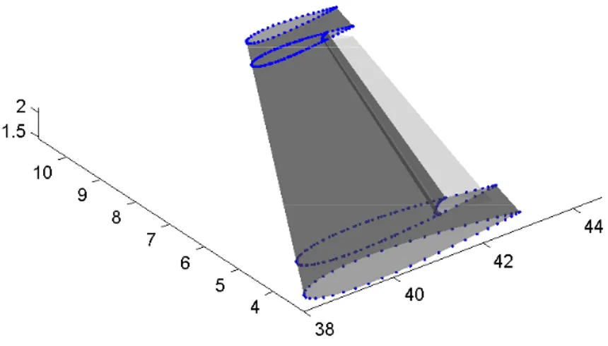
involved and the surface derivatives on them. To create a Wround feature at least 2 wings must be defined. In the Start Wing panel the user selects from a dropdown menu the first wing and the airfoil to be connected to the second wing. The same is done with the End Wing panel for the second wing. Pressing the Preview push-button will plot on a separate figure a preview of the skeleton and of the resulting interpolated surface in dark transparent gray, and the two wings that take part at the generation in light transparent gray, as shown in fig.1.33.
1.2.11
Viewing the Results
Every surface generated is passed to the Surfaces Viewer window and is automatically selected for plotting. The user can now select which features to plot and what kind of plot to perform. The options are:
1. Render : the surfaces are rendered in different color depending on the type of surface using a metal like look (fig.1.35).
Figure 1.33: The wround feature window
Figure 1.34: The Surface Viewer window
2. Render Shaded : the surfaces are rendered in different color depending on the type of surface using a metal-like look and a half transparent effect(fig. 1.36). 3. Three Plane View: the surfaces are rendered in gray using a metal-like look
1 – ASD: Aerodynamic Shape Design
Figure 1.35: Surface Viewing: Render
Figure 1.36: Surface Viewing: Render Shaded
1.37).
By default the plots are not symmetrized, and the trim lines calculated during surface generation are not shown. The user can turn on the symmetization or the trim lines plot by clicking on the corresponding checkbox (see fig.1.34). However, only surfaces are symmetrized, while trim lines are plotted only for the y > 0 plane.
Figure 1.37: Surface Viewing: Three-Plane View
1.3
ASD Surface Mesher
From the ASD main window it is possible to launch the ASD Surface Mesher on the selected features. Obviously the features selected must contain surface data. The ASD Surface Mesher is a GUI designed to help the user manage all the parameters and functions underlying the process of mesh generation. The ASD Surface Mesher sub-function are specifically designed to generate triangular meshes with maximum chord distance and maximum element size specified by user. The interface also enables the user to perform different tasks on the mesh, ranging from Delaunay flip to triangular-to-mixed mesh transform, plotting and analyzing meshes. In this section only a brief illustration is given, for more details on the surface mesher refer to [1], for more details on grid topics see also section 5.
The Mesh Data and Mesh stats panel (active only after a mesh has been ana-lyzed) summarize the mesh properties. The mesh generation controls are grouped in the Mesh Parameters panel. From this panel its possible to define and generate a mesh. The Max Chord Distance parameter specifies the maximum distance from the
1 – ASD: Aerodynamic Shape Design
Figure 1.38: ASD Surface MESHER, the interface window
real surface to the mesh (fig.1.39), whereas the Max Element side length parameter
Figure 1.39: Mesh parameters: max chord distance
specifies the maximum element side length. The Collapse Ratio can only assume values greater than 0 and lower than 0.5. When the conform mesh box is checked
the conform algorithm uses this value to decide whether to move a point on the interface of two surfaces or to add a triangle. The ratio is the maximum value of the ratio point_to_add_distance/segment_length that the user allows to move points. Above that value a new triangle is added. This conform procedure is only applied to the inlet/outlet and wingbody mesh creation, and will thus not affect all other surface meshes.
Figure 1.40: Mesh parameters: collapse ratio
The ASD Surface Mesher meshes all the surfaces separately, then trims the meshes created according to the trim lines calculated by ASD Surface Generator. The meshes so created might not be correctly connected at the interface of two surfaces (see fig.1.41). When correct mesh connection is desired the Conform Mesh box should be checked.
When a mesh is calculated, all the surfaces are meshed independently. All these partial meshes are stored inside the relative feature structure. At the end of the meshing procedure, whether it has been conformed or not, all the partial meshes are concatenated into one single mesh. Most of the following function work on this mesh, few of them work on the element mesh.
1 – ASD: Aerodynamic Shape Design
Figure 1.41: Non conform mesh and conform mesh
The Rebuild tri mesh function rebuilds the complete mesh starting from the mesh contained into single features. This is useful to recover the original mesh.
The set of tools within Plot Option Panel are used to plot the full mesh, calculate and plot the edges and plot the results of the mesh analysis. All these functions work on the full mesh and do not modify it. The interface is similar to the one of the new structured mesher (section 5.5) thus it won’t be reported here.
The Mesh Transform Panel groups all the mesh transform options. All the func-tions inside this panel work on the complete mesh and only if the type is “tri”. Triangular meshes are converted to mixed (quad-tri) meshes by recursively bonding together two adjacent triangles which meet the requested characteristics. The control parameters are the maximum angle between the triangles normal to allow union of the two triangles into one quadrilateral element, and the maximum value of skewness allowed for the resulting quadrilateral element. Finally, the Tri2mixed button starts the conversion, which modifies only the complete mesh.
The Tri Mesh Operations panel groups all the mesh operation options, which are mesh analysis, to perform a mesh geometric analysis, mesh symmetrization, in order to symmetrize the mesh taking care of normal reversing wherever needed, node
equivalence to perform a node equivalence based on the specified tolerance with the
intent of collapsing all the points that are closer, and mesh closure, to close open meshes with a simple triangulation. The last function is useful to prepare meshes for softwares that do not allow open surfaces.
(a) Open mesh (b) Closed mesh
Figure 1.42: Tri-mesh operation: closure of a mesh.
The Mixed Mesh Operations panel groups all the mixed mesh operation options, aimed to automatic LE and TE wake lines search. This functions are used when preparing an input file for an aerodynamic panel method, where wake separation lines must be specified into the code. And, finally Feature Operations panel groups the Delaunay Flip, which perform a cycle of Delaunay flips in 3D space (if the Full checkbox is selected the cycles are repeated until no flips are left), and the Align
Normal functions, which aligns the element normals according to the sign of the
global feature normal determined during surface generation.
1.4
The ASD tools
1.4.1
Airfoil Manager
Airfoil Manager is a graphical user interface (GUI) designed to manage airfoil
databas-es stored in .dat fildatabas-es. The interface is currently capable of reading a folder containing the .dat files, displaying it in a listbox and plotting the selected airfoil along with the information on the file and the airfoil. The interface can operate on plain coordinate file as well as labeled coordinate files, as long as the points are stored starting from the trailing edge and ending on the trailing edge itself.
1 – ASD: Aerodynamic Shape Design
(a) Mesh before Delaunay flip (b) Mesh after Delaunay flip
Figure 1.43: Feature operations: full Delaunay flip.
The only section accessible by the user the Plot Option panel, where the user can select if and how the airfoil must be interpolated and how many points must be used for interpolation. This number is the same number the airfoil is saved, so it does not only affect the quality of the plot, but also the quality of the exported airfoil .dat file. The options are among the original airfoil coordinates as loaded from the
.dat file, the original airfoil coordinates with the chord forced parallel to the x axis,
the interpolated airfoil with linear distribution and cosine distribution. The editable text box allows the user to set the number of points for the interpolated airfoil.
The airfoil attributes panel is used to estimate camber, thickness information of the currently selected airfoil, based on the interpolated curve calculated on the original points. There may be a little disagreement with the actual thickness and camber values.
In the airfoil info panel are collected all the information regarding the selected airfoil: the name and the number of points stored in the .dat file.
Figure 1.44: Airfoil Manager GUI
1.4.2
NACA Airfoil Generator
NACA Airfoil Generator is a graphical user interface (GUI) designed to create NACA
4-digit and NACA 5-digit airfoil series.
The interface gives the user the capability to explore different airfoils by simul-taneously plotting thickness distribution, camber line and the airfoil itself on two graphical windows. The tool is currently capable of dealing with 4-digit and 5-digit standard (non-modified) NACA airfoils such as, for example the NACA4415 or the NACA23012 airfoil.
The user could only introduce the name of the airfoil and the number of points to generate. This number is the same number the airfoil is saved, so it does not only affect the quality of the plot, but also the quality of the exported airfoil .dat file. The points are calculated every time the user changes any of the two editable texts,
1 – ASD: Aerodynamic Shape Design
Figure 1.45: NACA Airfoil Generator GUI
and are distributed along the chord using a cosine-law. For equations of the NACA 4 or 5-digit series refer to [5].
1.4.3
Section Sketcher
The interface gives the user the capability to create a section with any shape, or to explore a section in a database by plotting the section coordinates as stored in the
.dat file, on a graphical window. Finally, the interface includes a Save As command
to save the result as a plain coordinate .dat ASCII file.
The interface is very simple and consists of only one window. This window is divided in a plot box where the section is shown along with the current parametriza-tion, one modify box where the user can modify the section inserting, adding or moving some control points, one visualization box where the users decide the rep-resentation of the section, one zoom box containing the details about the zoom of the file representation, one interpolation box where the user controls interpolation parameter, one export box.
Figure 1.46: Section Sketcher GUI
all the points in the curve are checked if removable maintaining the curve into the prescribed tolerance. The Redistribute points redistributes the interpolation points of the NURBS uniformly in the parametric space. The number of points used in redistribution process is set by the user in the dialog box.
1.4.4
Flap Sketcher
Flap Sketcher is a graphical user interface designed to help defining 2-dimensional
mobile curves on different airfoils by means of NURBS. The interface gives the user the capability to create any Flap/Slat configuration starting from the base airfoil, or to modify an existing configuration.
The idea is to create a description of the mobile surfaces that is, to some extent, independent from the original airfoil it was created on. To achieve this, the mobile surfaces are saved in a parametric format and automatically adjusted to the loaded
1 – ASD: Aerodynamic Shape Design
Figure 1.47: Flap Sketcher GUI
airfoil.
The Flap/Slat creation process consists of 3 basic steps:
• select the base airfoil,
• draw the flap/slat lines using the sketch assist tools of the flap sketcher • position the center of rotation of every surface.
In the first step, an airfoil is easily loaded by means of the menu. Once loaded the airfoil is shown on both windows. The upper window shows the lines and should be used to sketch, while the lower window shows the results of the operations. Besides this, both windows can be used to enter points.
There are several methods to input the lines that define a flap/slat surface. Every line added modifies the flap configuration and the result is displayed on the lower window. There are 3 different types of lines, that differ essentially for the end derivatives.
The C type line is tangent to the airfoil surface and both end derivatives point towards the trailing edge. The first points to input are the ones on the airfoil border, upper and lower, then all the points that define the line between these two. The user can input an unlimited number of points in any order, but usually 3 to 5 are sufficient. In the lower window the user sees the result of the splitting. If the
free-hand radiobutton is selected the user can freely input the points that define the line,
while if the arc of parabola radiobutton is selected the user must input only one intermediate point, and the parabola arc will be automatically generated.
Figure 1.48: Flap Sketcher: C type line
The S type line is tangent to the airfoil surface with the upper end derivative pointing towards the trailing edge and the lower pointing towards the leading edge. The process is identical to the C type line, however a cubic curve instead of an arc of parabola is given.
The O type line is a closed line used to define those parts of the control surface that completely lay inside the airfoil. To define these type of surfaces the user must first provide the point that will be treated as a TE of the surface, then the one that will be treated as the LE, then all the points on the left and finally the points on the right. The sketch of this surface is currently only available in free-hand mode only.
1 – ASD: Aerodynamic Shape Design
Figure 1.49: Flap Sketcher: S type line
Figure 1.50: Flap Sketcher: O type line
To input the points is also available a coordinate mode, that asks the user to manually input the coordinates of the points.
Every line added is given a default name and it is listed on the left of the window. The program automatically creates the surfaces that are defined by the current lines, starting from the LE to the first line, from the second line to the third line and so
on.
To complete the flap/slat creation, all the movable surfaces must be assigned a hinge point; this is achieved by selecting the point directly on the plotting window, otherwise by entering the coordinates in a popup window.
1.5
ASD Limitations
ASD limitations are documented and reported in [1; 2]. However, different problems arises during program utilization in conjunction with other softwares. In fact, when exporting the surfaces generated from ASD to an IGES format, and then importing this file with the multi platform CAE/CAD/CAM commercial software CATIA, or other similar softwares, an unexpected difficulty occurs. Advanced softwares like CATIA and Pro/ENGINEER, being oriented also to automotive and industrial de-sign where the freeform surfaces should meet strict requirements to near perfect aesthetical reflection quality, implement a severe surface analysis. As will be shown in section 3.5, high quality surfaces require curvature and tangency alignment. On the other hand, ASD geometrical engine relies on an interpolation surface algorithm capable of generating surfaces with just tangency alignment. Thus, in the process of importing an ASD generated surfaces, the advanced softwares recognizes the cur-vature discontinuities, and splits the shape in a multitude of patches at the internal whom also the curvature is continuous.
On the visual side, this inconvenient could be overcome, at least on CATIA, by selecting the appropriate visualization filters (see fig.1.51 and 1.52). But, on the practical side, this split process create a multitude of entities which not only slow down the program, but cause the work to be impractical.
The most sever drawback arises when other programs import the CATIA or Pro/ENGINEER configuration in order to do some operations, like grid generation. A typical usage is the CATIA and GAMBIT pairing in order to create an high quality mesh for an accurate CFD analysis with FLUENT software, for example. When GAMBIT recognizes all the patches, the grid generation problem becomes prohibitive. Further, the CFD postprocessing is cumbersome: to know the forces
1 – ASD: Aerodynamic Shape Design
(a) Visualization option: shading with edges
(b) Visualization option: shading with edge without smooth edges
Figure 1.51: A surface generated with ASD and imported with CATIA. Note the patch subdivision.
acting on a wing, the patches should be merged. An optimization, which relies on automation, is thus not possible for grid generation and CFD analysis processes.
To overcome this first limitation, modifications on the geometric engine are need-ed. Referring to figure 1.53 and figure 1.54, the modifications should focus on the NURBS subblock.
Other main ASD limitation is the inability to generate a structured grid. In order to interface the grid generated from the internal mesher to a preliminary aerodynamic analysis program, like a panel method code, some restrictions on the mesh should be met. These programs, and in particulary Pan Air, require a structured grid as input geometry.
(a) Visualization option: shading with edges
(b) Visualization option: shading with edge without smooth edges
Figure 1.52: A surface generated with ASD and imported with CATIA. Note the patch subdivision.
Thus, close to the actual mesher, fig.1.55, a structured mesher module should join the grid generation process.
1 – ASD: Aerodynamic Shape Design
1 – ASD: Aerodynamic Shape Design
2
NURBS (Non Uniform Rational B-Spline)
Starting from a brief historical summary on CAGD (computer aided geometric de-sign), this chapter deals with parametric forms. For the most important of them, detailed mathematical model are reported, main characteristics are depicted, ben-efit and drawbacks are analyzed; especially for NURBS (non uniform rational B-Spline). Most outstanding algorithms aimed to NURBS manipulation are also briefly presented. Lastly, a short treatise on continuity is provided.
2.1
A Brief Historical Survey
The earliest recorded use of curves in a manufacturing environment seems to go back to early AD Roman times, for the purpose of shipbuilding. A ship’s ribs were pro-duced based on templates which could be reused. Later Venetians perfectionate these technique. Drawing became popular only in the 1600s in England, the classic spline was probably invented then. This connection between drawing and manufacturing in shipbuilding was the earliest use of constructive geometry to define free-form shapes. Another keypoint originated in aeronautics, with Liming (NAA, North American Aviation): he realized that to store a design in terms of numbers was more efficient instead of manually traced curves. Thus he translated the classical drafting con-structions into numerical algorithms. Liming’s work became very influential in the 1950s when it was adopted by U.S. aircraft companies.
2 – NURBS (Non Uniform Rational B-Spline)
The turning point was the advent of numerical control in the 1950s: machining of 3d shapes out of blocks of wood or steel became reality. Soon was found the need-ing of adequate software, in terms of producneed-ing a computer compatible description of shapes. The most promising description was found to be in terms of parametric surfaces. At that time the theory of parametric surfaces was well understood in differential geometry, but their potential for the representation of surfaces in a Com-puter Aided Design (CAD) environment was not known at all. This exploration can be viewed as the origin of Computer Aided Geometric Design (CAGD) 1. Only large
corporations could afford the computers capable of performing the calculations, so the developments were internal at each company and kept secrets.
In the 1960s-1980s one of the major contribution to CAGD development was the work of of B´ezier (at Renault), who defined a particular polynomial parametric form, milestone for the subsequent development; this leads in 1971 to UNISURF, car body design and tooling.
Stand-alone from B´ezier’s work was mathematician de Casteljau activity at Cit-ro¨en. He adopted the use of Bernstein polynomials for his curve and surface defini-tions from the very beginning, together with what is now known as the de Casteljau algorithm; another of the breakthrough insight of his work was to use control poly-gons, a technique that was never used before. After it was found that his parametric curve is mathematically identical to B´ezier’s one. His work was publicized only in 1967.
In the US, the development was linked mainly to the aerospace industry. Ferguson (at Boeing) used piece cubic curves together so that they formed composite curves which were overall twice differentiable; these curves, referred as spline curves could easily interpolate to a set of points. The meaning of the term spline curve has since undergone a subtle change. Instead of referring to curves that minimize certain functionals, spline curves are now mostly thought of as piecewise polynomial (or rational polynomial) curves with certain smoothness properties. Ferguson’s first works was printed in 1964.
1This term was introduced by Barnhill and R. Riesenfeld in 1974, during the first famous conference on that topic, at the University of Utah.
Coons (MIT researcher and FORD consultant) developed the patch theory using cubic piecewise polynomials in the Hermite form. Coons devised a simple formula to fit a patch between any four arbitrary boundary curves. His famous report were publicized in the 1967. Improvements about this topic (called transfinite
interpo-lation) were done by Gordon (at General Motors) who developed a generalization,
capable of interpolating a rectangular network of curves, and Gregory.
De Boor (at General Motors) was the first to introduce the tensor product surface. He also was the first to use B-Splines (short for Basis Splines) as a tool for geometric representation. The recursive evaluation of B-spline curves is due to him and is now known as the de Boor algorithm: it is based on a recursion for B-splines. It was this recursion that made B-splines a truly viable tool in CAGD. Before its discovery, B-splines were defined using a tedious divided difference approach which was numerically very unstable.
Spline functions are important in approximation theory, but in CAGD, para-metric spline curves are much more important. These were introduced in 1974 by Riesenfeld and Gordon who realized that de Boor’s recursive B-spline evaluation was the natural generalization of the de Casteljau algorithm. B-spline curves include B´ezier curves as a proper subset and soon became a core technique of almost all CAD systems. A first B-spline-to-B´ezier conversion was found by W.Boehm. Sev-eral algorithms were soon developed that simplified the mathematical treatment of B-spline curves.
The generalization of B-spline curves to NURBS has become the standard curve and surface form in the CAD/CAM industry. They offer a unified representation of spline and conic geometries: every conic as well as every spline allows a piecewise rational polynomial representation. The development at Boeing is exemplary for the emergence of NURBS. The company realized that different departments employed different kinds of geometry software; worse, those geometries were incompatible. Thus NURBS were adopted as a standard since they would allow a unified geometry representation. Companies such as Boeing, SDRC, or Unigraphics soon initiated
2 – NURBS (Non Uniform Rational B-Spline)
making NURBS an IGES standard 2.
In the last twenty-thirty years the technological development brings CAD tools area of application outside industry and brought them till inside the medium user computer. Such a change hauled with him CAGD research and development.
Today in totally different from industrial areas arises typical geometric model-ing problems. For example, subjects like geology, weather forecast, medicine are concerned with surface fitting problems.
For a more detailed discussion about the history and the development of CAGD refer to [6; 7].
2.2
Curve and Surface Basics
The two most common methods of representing curves and surfaces in geometric modeling are implicit equations and parametric functions. Sometimes other rep-resentations can be used (for example explicit representation), but the previously mentioned are predominant in the academic, industrial and commercial world. For more details refer to [7; 8; 9].
2.2.1
Implicit and Parametric Forms
Implicit Forms
In the implicit forms, one or two equation describes a relation between the spatial coordinates of the points of the form. For an implicit surface: f (x,y,z) = 0. Every form has his unique representation, a part for a multiplier constant. The description of a curve in the three dimensional space is obtained as intersection of two implicit surfaces: f1(x,y,z) = f2(x,y,z) = 0.
2Initial Graphics Exchange Standard, developed to facilitate geometry data exchange between different companies.
Parametric Forms
In the parametric forms, each of the coordinates of a point is represented separately as an explicit function of one or more independent parameters. For a surface: C(u,v) = (x(u,v),y(u,v),z(u,v)), with u and v being the two independent parameters: hence, it is essentially a mapping of a domain D ⊂ R2 in R3 (usually the domain D is
normalized to [0 1] x [0 1] ). The description is not unique for a form. In the curve case, the independent parameter is only one.
2.2.2
Advantages and Disadvantages
There is no answer to the question of which form is better. Every form can be more appropriate, depending from the application. Anyway, a comparison follows about capabilities and limits of the previously mentioned forms:
• The parametric form is more suited for simultaneous two and three
dimension-al representation: adding or removing third coordinate switches between the cases. On the other hand implicit aren’t so flexible: a curve in two-dimensional spaces is represented with an implicit equation, but the generalization to the three dimensional space need adding, apart from the third coordinate, also another implicit equation.
• It is cumbersome to represent bounded curve segments or surface patches
with the implicit form. However, boundness is built into the parametric form (through the bound of the parameter value). On the other implicit forms are well suited for unbounded geometry; the opposite states for parametric forms
• Parametric form introduce a direction; for the curves the natural direction
should be defined concordant to the parameter. Hence, it is easy to generate ordered sequences of point along a parametric curve, and meshes of points on surfaces.
• The parametric form is more natural for designing and representing shape
2 – NURBS (Non Uniform Rational B-Spline)
considerable geometric significance. This leads to an intuitive design method and numerically stable algorithms with a distinctly geometric flavor.
• The complexity of many geometric operations depends greatly on the method
of representation. For example, to compute a point on a curve or surface is difficult in the implicit form, but determine if a given point lies on the curve or surface is difficult in the parametric form.
• Sometimes in the parametric form one must deal with anomalies, unrelated to
true geometry. A classic example is the unit sphere: here the parametric cal-culations of the pole is critical, even if geometrically this points aren’t different from the other points on the surface.
Since we are concerned almost exclusively with bounded surfaces, computer use and the geometric insight of the coefficient is important, the parametric form will be the preferred one.
2.2.3
Requirements for the parametric forms
In order to fulfill the CAD/CAE demands, a parametric representation should be efficiently implemented on the computer, should allow the description of the geome-tries of interest and should allow the local post-editing of part of that shape (that is modify, after created, the shape in a specific point should not modify the rest of the shape). In particular the choice would be restricted to the representation capable of satisfying the following points:
1. ability to describe geometries like straight lines, continuous curves and piece-wise curves, aerodynamic surfaces with mathematical accuracy
2. capability of easy processing in a computer contest, in particular: (a) easy and efficient points and derivatives evaluation,
(b) calculation insensitivity to trunk and round-off errors, (c) small memory allocation request for storage;
2.2.4
Power Basis Form of a curve
A widely used class of functions is the polynomials. Although they satisfy the second and third point of the previous list, they fail to represent precisely a number of im-portant curves. There are two common methods of expressing polynomial functions, the first is power basis (the other one is B´ezier). A nth-degree power basis curve is given by: C(u) = [x(u),y(u),z(u)]T = n X i=0 aiui with 0 ≤ u ≤ 1 (2.1)
where ai are vectors, u the parameter. In matrix form it holds:
C(u) = [A] · [u] = [ai]T[ui] (2.2)
where A = [a0 a1 . . . an] and ui = [1, u, u2, u3...]T are the basis functions. The
power basis form has the following disadvantages:
• is not well suited with interactive shape design; the coefficients ai carry very
little geometric insight about the shape of the curve;
• the algorithms for processing power basis (e.g., Horner’s method [8]) are
alge-braic rather than geometric oriented;
• the algorithms are prone to round-off error if the coefficients vary greatly in
magnitude.
2.2.5
B´
ezier Curves
The B´ezier curves were developed independently by B´ezier (at Renault) and de Casteljau (at Citro¨en). From a mathematical point of view they are exactly the same as power basis, but they remedy the latter’s shortcomings. A nth-degree B´ezier curve is defined by
C(u) =
n
X
i=0
2 – NURBS (Non Uniform Rational B-Spline)
where Pi, the geometric coefficients, are the control points, and Bi,n(u), the basis (or
blending) functions, are the classical nth-degree Bernstein polynomials, given by:
Bi,n(u) =
n! i!(n − i)! u
i (1 − u)n−i (2.4)
The union of the control points is called control polygon. In addition B´ezier curves
0 P 0 P 1 P 1 P 3 P0=P3 P 2 P 2 Control Polygon Control Polygon
Figure 2.1: Two examples of cubic B´ezier curves.
are invariant under the usual transformations such as rotations, translations and scalings; that is, one applies the transformation to the curve by applying it to the control polygon.
In any representation scheme, the choice of the basis functions determines the geometric characteristics. These functions have these properties:
P.1.1 nonnegativity: Bi,n(u) ≥ 0 for all i,n and 0 ≤ u ≤ 1;
P.1.2 partition of unity: Pni=0Bi,n(u) = 1 for all 0 ≤ u ≤ 1;
P.1.3 B0,n(0) = Bn,n(1) = 1;
P.1.4 Bi,n(u) attains exactly one maximum on the interval [0,1], exactly at u = ni ;