i
Università degli Studi di Padova
Dipartimento di Scienze Statistiche
Dipartimento di Scienze Economiche
Corso di Laurea Magistrale in
Scienze Statistiche
INVESTING FOR THE LONG RUN:
PREDICOR VARIABLES AND LOSS AVERSION
Relatore: Ch.mo Prof. Massimiliano Caporin
Dipartimento di Scienze Economiche
Laureando: Alessandra Porra
iii
Contents
Introduction ... vi
1. Short run portfolio allocation ... 1
1.1Introduction ... 1
1.1 Financial market returns from 1802 ... 1
1.2 Asset returns ... 4
1.2.1 Portfolio returns ... 6
1.2.2 Excess returns and risk-free asset ... 7
1.3 Expected Utility Theory ... 9
1.4 Mean-Variance Analysis ... 12
1.4.1 The form of the utility function ... 16
1.4.2 Limitations of the Mean-Variance Model ... 17
1.5 The holding period ... 19
1.5.1 Long-run portfolio choice ... 20
2. Portfolio allocation with parameter uncertainty ... 22
2.1 Introduction ... 22
2.2 Parameter uncertainty ... 22
2.3 Data set... 24
2.3.1 Preliminary analysis ... 25
2.4 Long horizon portfolio allocation ... 32
2.4.1 Sampling process ... 36
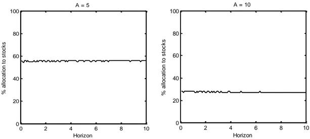
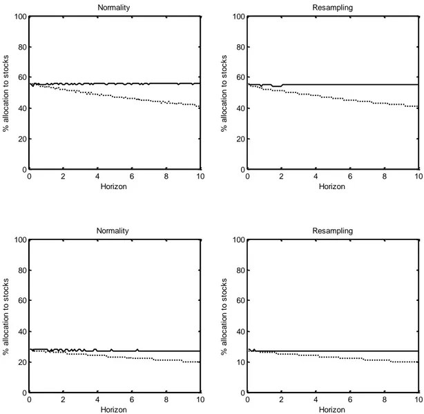
2.5 Results ... 37
2.6 Resampling ... 41
2.6.1 Results ... 42
3 Portfolio allocation with predictable returns ... 44
3.1 Introduction ... 44
3.2 Returns predictability ... 44
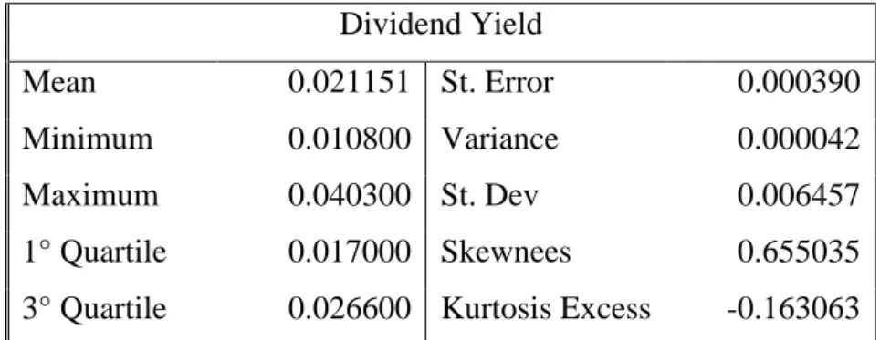
3.3 Predictor variable: dividend yield ... 45
3.3.1 Preliminary Analysis ... 46
3.4 Long horizon predictability and parameter uncertainty ... 49
iv
3.6 Long horizon portfolio allocation ... 53
3.6.1 Sampling process ... 57
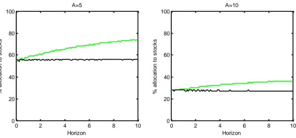
3.7 Results ... 58
3.8 The role of the predictor variable ... 64
4 Portfolio allocation with parameter uncertainty: two risky assets ... 67
4.1 Introduction ... 67
4.2 An extra risky asset: the bond index... 67
4.2.1 Preliminary analysis ... 69
4.3 Model with two risky assets ... 72
4.4 Long horizon portfolio allocation ... 74
4.4.1 Sampling process ... 78
4.5 Results ... 79
5 Portfolio allocation with predictable returns and five predictor variables ... 84
5.1 Introduction ... 84
5.2 Stock and bond predictability ... 84
5.3 Predictive variables ... 85
5.3.1 Vix index ... 86
5.3.2 Term spread ... 89
5.3.3 Credit spread ... 92
5.3.4 Risk-free asset ... 95
5.3 Predictability analysis model ... 95
5.4 Results ... 98
5.5 The role of the predictor variables ... 105
5.6 Other samples results ... 108
5.6.1. Sample 1990-2000 ... 108
5.6.2. Sample 2002-2006 ... 109
5.6.3 Sample 2007-2012 ... 111
6 Portfolio allocation under loss aversion ... 114
6.1 Introduction ... 114
6.2 Critiques to the Expected Utility theory ... 114
6.3 Behavioral Finance ... 116
6.4 Prospect theory ... 118
6.5 Long horizon asset allocation ... 121
6.6 Results ... 123
v Appendix A ... 130 Sample 1990 – 2000 ... 130 Sample 2002 – 2006 ... 132 Sample 2006 - 2012 ... 134 Appendix B ... 136 Bibliography ... 153
vi
Introduction
Portfolio choice problems are the leading edge of financial research. The portfolio theory underlying an investor’s optimal portfolio choice, pioneered by Markowitz’s
vii Mean-Variance Anlysis (1952), is by now well comprehended. The reborn interest in portfolio choice problems follows the relatively recent empirical evidence of time-varying return distributions (predictability and conditional heteroskedasticity). The purpose of this work is indeed to examine the effects of predictability for an investor trying to take portfolio allocation decisions. According to Samuelson (1969) and Merton (1969), when asset returns are i.i.d., an investor who rebalances his portfolio optimally and whose preferences are described by a power utility function, should choose the same asset allocation regardless of the investment horizon. However, considering the growing evidence of predictability in returns, the investor’s horizon may no longer be unimportant. We therefore address this issue of portfolio choice from the perspective of horizon effects: “Given the demonstration of predictability in asset returns, should a long horizon investor allocate his wealth differently from a short-horizon investor?” (Barberis, 2000)
Our work draws on Nicholas Barberis’ paper (2000) about long run predictability of asset returns. In his work he studies the effects of predictability for an investor making sensible portfolio choices. He analyzes portfolio choice in discrete time for an investor with power utility function over terminal wealth, employing two assets: a stock index and a risk-free asset. In order to examine how predictability affects portfolio choices he compares the allocation of an investor who does not recognize predictability, that is when asset returns are described by a i.i.d. model, to that of an investor who takes predictability into account. In particular he uses only one predictor variable in order to describe asset returns’ dynamics, the dividend yield. He finds that predictability in asset returns leads to strong horizon effects, involving a much higher allocation to stocks for a long-horizon investor than for a short-horizon investor, this being because predictability makes stocks look less risky at long horizons.
In our work we try to understand if a risk averse investor, who decides today how to invest his wealth and does not change the allocation until the predetermined maturity, distributes his wealth differently for long horizons compared to short horizons. We firstly focus on studying the predictive power of only one variable, the dividend yield, for stock returns. Afterwards, we devote most of our work to examining in what way the optimal portfolio allocation changes when investors have the
viii
opportunity to choose how to allocate their wealth among three different assets, instead of the previous two: a stock index, a bond index, and a risk-free asset. We then investigate the predictability of excess stock and bond returns, availing ourselves of a set of five predictor variables gathered from the financial literature. Particular attention is paid to estimation risk, which can be defined as the uncertainty about the true values of model parameters. We analyze estimation risk in order to take into account the uncertainty about the true predictive power of predictor variables, that sometimes could be weak. This approach constitutes therefore a middle ground between rejecting the null hypothesis of returns predictability, and analyzing the problem taking the parameters as fixed and known precisely.
In addition to what Barberis handled in his paper, we then devote our attention to introducing an alternative method to the Expected Utility approach, that is the Prospect Theory developed by Kahneman and Tversky (1979), whose goal is to capture people’s attitudes to risky gambles as parsimoniously as possible. According to this theory a value function replaces the usual utility function, in particular the loss aversion utility function explains the investors’ behavior of being risk averse for gains and risk seeking for losses. Moreover it describes the principle of loss aversion, according to which losses loom larger than corresponding gains. Our purpose is therefore to examine how the optimal portfolio allocation changes depending on whether the function employed to describe investors’ preferences over wealth is a power utility function or a loss aversion function.
Regarding the application we evaluate a vector autoregressive model in order to explain the time-variation in asset returns throughout the predictor variables. Afterwards uncertainty about the model parameters is incorporated by the posterior distribution of the parameters given the data
The purpose of the first chapter is to explain in detail some concepts and ideas used throughout the work. After a brief description of financial markets returns over the last two centuries, we define the notions of asset return, excess return and risk-free rate.
The Expected Utility Theory and Mean-Variance Analysis are then illustrated. Finally we consider the case handled by Samuelson and Merton, when long-term
ix investors act myopically, choosing the same portfolio as short-term investors, and we specify the main approaches an investor can adopt.
In the second chapter attention is paid to the estimation risk, in other words we study the optimal portfolio allocation assuming that parameters are not known precisely. Our purpose is to understand how parameter uncertainty alone affects portfolio choice. According to a Bayesian approach, we define the posterior distribution of the model parameters given the data, and integrating over the uncertainty in the parameters captured by the posterior distribution, we construct predictive distribution for future returns, conditional only on observed data, and not on any fixed parameter value. The model implemented is then applied to a real dataset. Finally we illustrate the results obtained both assuming that excess returns have a normal distribution and adopting a resampling approach in order to understand if the assumption of normality attributed to assets returns affects the optimal portfolio allocation.
The third chapter focuses on how predictability affects portfolio choice. For the initial study of predictability of excess stock returns only one variable is taken into account, the dividend yield. A vector autoregressive model of the first order with some restrictions on its parameters is defined in order to examine how the evidence of predictability in asset returns affects optimal portfolio choice. The model is then applied to a real dataset and the results of the optimal portfolio allocation for different investment horizons are presented for a buy-and-hold investor who is risk-averse. Finally, the results obtained considering different initial values of the dividend yield are reported in order to understand the role of the predictor variable We devote the fourth and fifth chapters to develop some extensions to the model implemented in chapters 2 and 3. We study the optimal portfolio allocation when investors have the opportunity to choose how to invest their wealth among three different assets: a stock index, a bond index, and the risk-free asset . The purpose of the fourth chapter is similar to the one of the second chapter, that is to understand how estimation risk alone affects portfolio choice. Some changes to the original model are therefore implemented in order to define an appropriate framework, which allows to us to examine the impact of parameter uncertainty when the investor can allocate his wealth among three different assets instead of two assets. The model
x
we implemented is then applied to a real dataset, and the results of the optimal portfolio allocation for a buy-and-hold investor who is risk-averse are illustrated. In the fifth chapter we focus on the study of predictability of excess stock and bond returns, and in order to do that, we avail ourselves of a set of five predictor variables. The model is similar in essence to the one we implement in the third chapter, a vector autoregressive model of the first order with some restrictions on its parameters. Applying it to a real dataset, we examine how the evidence of predictability affects portfolio choice when investors can choose to allocate their wealth between a stock index, a bond index and a risk free asset.
Finally, in the fifth chapter, after having related the main critiques to the Expected Utility Theory we bring up some experimental evidence that led to the emergence of Behavioral Finance. We then introduce the Prospect Theory, a behavioral economic theory that tries to describe investors’ real-life choices, and we investigate how the optimal portfolio allocation changes when investors’ preferences are described by a loss aversion utility function.
1
Chapter 1
Short run portfolio allocation
1.1 Introduction
The first one, is primarily a review chapter, whose purpose is to illustrate some ideas and concepts used throughout our work.
We firstly make a brief description of financial markets returns over the last two centuries. Afterwards we define the concept of asset return and illustrate some returns’ appealing statistical properties. In this paragraph the meanings of risk-free rate and excess return are also explained.
The third paragraph is devoted to the Expected Utility Theory, which is used in order to describe economic agents’ decisions under uncertainty.
In the fourth paragraph it is described the Mean-Variance Analysis, a portfolio choice theory whose main objective is to define the optimal portfolio allocation in the short-run; and its limitations are then given.
Finally we consider the case handled by Samuelson and Merton, when long-term investors act myopically, choosing the same portfolio as short-term investors.
1.1 Financial market returns from 1802
Risk and return are the fundamental blocks of finance and portfolio management. Once the risk and expected return of each asset are specified, modern financial theory can help investors define the best portfolios. But the risk and return on stocks and bonds are not physical constants. Despite the overwhelming quantity of historical data, one can never be certain that the underlying factors that generate asset prices have remained unchanged. One cannot, as in the physical sciences, run repeated controlled experiments, holding all other factors constant while estimating the value of the parameter in question.
2
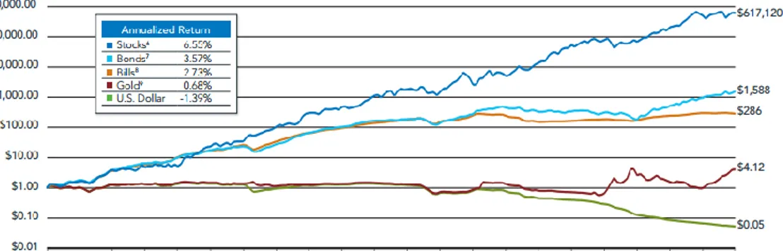
However, one must start by analyzing the past in order to understand the future. In the next few paragraphs we carry a short analysis of past returns on stocks and bonds over the last two centuries. During this two-century period great changes have revolutionized the United States. The United States firstly made a transition from an agrarian to an industrialized economy and then became the main political and economic power in the world. Modern times led to the 1929 to 1932 stock collapse, the Great Depression, and the postwar expansion. The story is illustrated in Figure 1.1. It displays the real total return indexes for stocks, long and short-term bonds, gold, and commodities from 1802 through 2011. Since the focus of every long-term investor should be the growth of purchasing power that is, monetary wealth adjusted for the effect of inflation, the data in the graph are constructed by taking the dollar total returns and correcting them by the changes in the price level. Total return means that all returns, such as interest and dividends and capital gains, are automatically reinvested in the asset and allowed to accumulate over time
Figure 1.1: Total real return indices, 1802 through June 2012
It can be easily seen that the total real return on equities dominates all other assets and also shows remarkable long-term stability. Indeed, despite extraordinary changes in the economic, social, and political environment over the past two centuries, stocks have yielded about 6.6 percent per year after inflation. The wiggles on the stock return line represent the bull and bear markets that equities have suffered throughout history. The short-term fluctuations in the stock market, which appear so large to investors when they occur, are insignificant when compared to the upward movement of equity values over time. The long-term perspective radically changes one’s view of the risk of stocks.
3 In contrast to the remarkable stability of stock returns, real returns on fixed-income assets have declined considerably over time. Until the twenties, the annual returns on bonds and bills, although less than those on equities, were significantly positive. But since those years, and especially since World War II, fixed-income assets have returned little after inflation.
Must however be said that in the real world investors consume most of the dividends and capital gains, so that the growth of the capital stock is not greater than the economy’s rate of growth even though the total return on stocks is substantially higher. It is rare for anyone to accumulate wealth for long periods of time without consuming part of his or her return. The stock market has the power to turn a single dollar into millions by the perseverance of generations, but few will have the patience or desire to suffer the wait.
Although it might appear to be riskier to accumulate wealth in stocks rather than in bonds over long periods of time, precisely the opposite seems to be true: there is indeed evidence that the safest long-term investment for the preservation of purchasing power is a diversified portfolio of equities.
Indeed, according to the data Siegel(1994) availed himself of in his analysis , standard deviation, that is the measure of risk used in portfolio theory and asset allocation models, is higher for stock returns than for bond returns over short-term holding periods, however, once the holding period increases, stocks become less risky than bonds. The standard deviation of average stock returns falls nearly twice as fast as for fixed income assets as the holding period increases.
Theoretically the standard deviation of average annual returns is inversely proportional to the holding period if asset returns follow a random walk. But the historical data show that the random walk hypothesis can not be maintained for equities. Indeed the actual risk of stock declines far faster than the predicted rate under the random walk assumption. All that highlights one of the most relevant factors to be considered in making investment choices, that is the holding period. Although the dominance of stocks over bonds is readily apparent in the long run, it is also important to note that in the short run, stocks outperform bonds or bills only about three out of every five years according to Siegel’s research. The high
4
probability that bonds and even bank accounts will outperform stocks in the short run is the primary reason why it is so hard for many investors to stay in stocks.
After a brief explanation of the main concepts and tools that will be used throughout our work, we will dedicate the next chapters to the exploration of the critical idea of how the holding period can affect the optimal allocation decision of an investor. We will firstly consider an investor who is allowed to choose how to invest his wealth only between a risk-free asset and a stock index, and afterwards we will add to the assets he can avail himself of a bond index.
1.2 Asset returns
When an empirical analysis in carried out, it is very important to use data whose type can supports the pursued objectives. Most financial studies involve returns instead of asset prices. There are at least two reason to contemplate returns rather than prices. Firstly, for the average investor, financial markets may be considered close to perfectly competitive, so that the size of the investment does not affect prices changes. Therefore, the return is a complete and scale-free summary of the investment opportunity. Secondly, returns have more attractive statistical properties than prices, such as stationarity and ergodicity
There are, however, several definitions of asset returns, we discuss some of them, that will be used throughout our work.
We denote byPt the price of an asset at time t . We assume for the moment that the asset pays no dividends.
One-Period Simple Return
Holding the asset for one period from date t1 to date t would result in a simple gross return : 1 1 t t t P R P , (1.1)
5 The corresponding one-period simple net return or simple return is:
1 1 1 1 t t t t t t P P P R P P . (1.2) .
Continuously Compounded Return
The natural logarithm of the simple gross return of an asset is defined as the continuously compounded return or log return:
1 1 log(1 ) log t , t t t t t P r R p p P (1.3) where pt logPt.
Continuously compounded returnsrt enjoy some advantages over the simple net returns Rt. First statistical properties of log returns are more tractable, indeed it has not any lower bound and it is therefore compatible with the hypothesis of Normality.
If r has normal distribution with meant mu and variance2 , the simple return
has lognormal distribution with mean
2 2 (1 t) E R e and variance 2 2 2 (1 t) ( 1)
Var R e e . Secondly, when we consider multiperiod returns:
1 1
1 1
1 1
( ) log(1 ( )) log((1 ) (1 )...(1 )
log(1 ) log(1 ) ... log(1 )
... , t t t t t k t t t k t t t k r k R k R R R R R R r r r (1.4)
Thus, the continuously compounded multiperiod return is simply the sum of the continuously compounded one-period returns involved. However, the simplification is more in the modeling of the statistical behavior of asset returns over time, indeed the previous assumption of normality hold true for multiperiod returns as well, since the sum of normally distributed variables is also normally distributed.
Dividend Payment
If an asset pays periodic dividends, the definitions of asset returns must be modified. Denote byD the asset’s dividend payment between dates t t1 and t, and by P the t
6
asset’s price at the end of period t . Thus, dividend is not included inP . Then the t simple net return and continuously compounded return at time t may be defined as
1 1
1 and log( ) log( ).
t t t t t t t t P D R r P D P P (1.5)
Note that the continuously compounded return on a dividend-paying asset is a nonlinear function of log prices and log dividends. However, when the ratio of price to dividends is not too variable , this function can be approximated by a linear function of log prices and dividends.
Throughout our work we will use continuously compounded returns. Continuous compounding is usually preferred when the focus of interest is the temporal behavior of returns, since multiperiod returns can be computed overtly. Conversely, it is common to use simple returns when a cross-section of assets is being studied.
1.2.1
Portfolio returnsAn investor’s portfolio can be defined as his collection of investment assets where he allocates his wealth. Denote byR the simple return connected with the asset it i , belonging to a portfolio counting N assets, and by i its weight in the portfolio. The simple return on a portfolio consisting of N assets is a weighted average of the simple net returns of the assets involved, where the weight on each asset is the percentage of the portfolio’s value invested in that asset. If portfolio p places weight
ip
on asset i, then the simple return on the portfolio at time t , Rpt, is related to the
returns on individual assets R , by it
1 N pt ip it i R R
where 1 1 N ip i
.Continuously compounded returns of a portfolio, unfortunately, do not have the above convenient property. Since the continuously compounded return on a portfolio is the logarithm of this linear combination, that is not equal to the linear combination of logarithms, in other words:
1 N pt ip it i r r
7 Moreover, the sum of log-normal distributions is not defined as a log-normal. In empirical applications this problem is usually minor. When returns are measured over short intervals of time, and are therefore close to zero, the continuously compounded return on a portfolio is close to the weighted average of the continuously compounded returns on the individual assets:
1 N pt ip it i r r
.1.2.2
Excess returns and risk-free assetFor the analysis that will be carried out later it is necessary to refer to a risk-free asset. The return on a risk-free asset may be defined as theoretical return of an investment with no risk of financial loss. The assumption is based on the evidence that in the market it is possible to find an asset that has a sure and well-known ex ante return. In practice, these assets are usually short-term government bonds of absolutely reliable countries, money market funds, or bank deposit. Formally, the risk-free random variable has constant expected value and a variance equal to zero. But it may appear risky since its returns can fluctuate over time and its variance move usually away from zero. Nevertheless their variability is minimal compared to the one of the risky assets and therefore can be well approximated to zero.
Since the risk free return can be obtained with no risk, it is implied that any additional risk taken by an investor should be rewarded with an higher return than the risk-free one. We measure the reward as the difference between the expected return on the risky asset and the risk-free rate. This difference is defined as the risk premium on common stocks.
It is often convenient to handle an asset’s excess return, in place of the asset’s return. Excess return is defined as the difference between the asset’s return and the return on some reference asset, where the reference asset is usually assumed to be the risk-free one. In the next equation, z contains the simple excess return on the risky asset it i relative to the risk-free asset.
it it
8
where rf specifies the risk-free return.
An investor could choose to invest a portion of his wealth in the risk-free asset, as well as in the N risky assets. If you specify with 0 the portfolio’s share of wealth invested in the risk-free asset, the portfolio return will then be:
0 , where 0 1, p f r r ω'r i'ω (1.7) alternatively ( ) , p f f r r ω' rr i (1.8)
where (rrfi)z, vector of excess returns.
Subtracting rf to both members of the expression above, we can obtain the portfolio excess return formula as function of risky assets’ excess return.
p
z ωz (1.9)
Here the weight vector does not sum to 1, since ω only represents the proportion invested in risky assets.
Since the risk-free random variable is assumed to have a constant mean and a variance equal to zero, the riskiness of risky assets is often measured by the standard deviation of excess returns. However, due to rf fluctuation over time, excess returns sample variances and covariances are not equal to returns’. Nevertheless the fluctuations of the risk-free assets are negligible compared with the uncertainty of stock market returns, the difference between the two variances will thus be small. Most of the time this condition is observed and the difference between the empirical variances of
r
andz
is not significant.The majority of economic models is based on hypothesis, not always verified, that return and excess return are independent realization from the same multivariate normal distribution.
9
1.3 Expected Utility Theory
Uncertainty plays a remarkable role in the investors’ processes of taking decisions. Since the future is unknown, investors make their choice within an uncertain overall framework, where every action carries different consequences depending on the state of nature that it will come true. Each state of nature has its own probability of success, and therefore they have a specific probability distribution.
Economic agents’ decisions under uncertainty can be represented as the choice of a particular prospect within a set of alternatives. In the case where individuals do not bother about the risk related to the choice of an uncertain prospect, their decisions are driven solely by the expected value criterion , which takes into account only the sizes of the payouts and the probabilities of occurrence. The alternative with the highest expected value will then be chosen. However, most people are not indifferent to the risk. Intuitively, one would rank each prospect as more attractive when its expected return is higher, and lower attractive when its risk is higher. But when risk increases along with return, the most attractive portfolio is not easy to be found anymore. How can investors quantify the rate at which they are willing to trade off return against risk? In situations involving uncertainty (risk), individuals act as if they choose on the basis of expected utility, the utility of expected wealth, rather than expected value.
Economists use Expected Utility Theory in order to explain decisions taken under uncertainty. This perspective, which focuses on man as a rational and predictable being in his actions, was developed in 1947 by Neumann and Morgenstern and has been widely accepted and applied as a model of economic behavior. According to this theoretical model, individuals, who are required to choose between several options, do not evaluate financial quantities depending on their amount, but on the satisfaction they subjectively confer on them. Investors can assign a welfare, or utility, score to competing investment portfolios based on the expected return and risk of those portfolios. The utility score may be viewed as a means of ranking portfolios, resulted from a criterion of personal choice, therefore it will depend on preferences of investors in a specific moment or situation. Higher utility values are assigned to portfolios with more attractive risk-return profile.
10
This theory allows us to study individual preferences, which are represented by a utility functionu , which is defined barring a monotonic increasing transformation. This function has two properties: it must respect the preferences order of the individual and it must be increasing, that is it must have positive marginal utility of wealth, since it is reasonable to confer more utility to greater payoffs.
Given a function u x( )where x corresponds to the wealth in t1 and assuming
'( ) 0
u x (rational investor), the expected utility of wealth result from
1 [ ( )] ( ) S i i i E u x p u x
(1.10) where 1 1 S i i p
and S are the states of nature.Investors choice criteria among several risky alternatives are always based on the expected utility result. Rational individuals choose the option that maximize their utility, on the basis of the expected utility rather than expected value of the outcomes. Therefore the preferred alternative depends on which subjective expected utility is higher. Different people may take different decisions because they may have different utility functions or different beliefs about the probabilities of varied outcomes.
Asked to choose between two prospects, a risk-free one, with sure return R, and a risky one with expected return equal to R, investors always compare u E x( [ ]) and
[ ( )]
E u x .
A risk averse individual would prefer to receive a certain return R rather than having an uncertain prospect whose expected value corresponds to R. He is therefore willing to give up a part of income in exchange for a sure outcome, since he considers uncertainty as a negative element. Financial analysts generally assume investors are risk averse in the sense that, if the risk premium were zero, people would not be willing to invest any money in stocks. A risk-averse investor penalizes the expected rate of return of a risky portfolio by certain percentage to account for the risk involved. The greater the risk, the larger the penalty. In theory, then, there must always be a positive risk premium on stocks in order to induce risk-averse
11 investors to hold the existing supply of stocks instead of placing all their money in risk-free assets.
In contrast to risk-averse investors, risk-neutral investors judge risky prospectus solely by their expected rates of return. The level of risk is irrelevant to the risk-neutral investor, meaning that there is no penalty for risk.
A risk lover is willing to engage in fair games and gambles; this investor adjusts the expected return upward to take into account the pleasure of confronting the prospect’s risk. Risk lovers will always take a fair game because their upward adjustment of utility for risk gives the fair game a higher utility than the risk-free investment.
The concept of risk aversion is useful to estimate risk effects in individuals’ satisfaction level and in their preferences.
Risk attitude is directly related to the curvature of the utility function:
A risk averse individual has concave utility function. Moreover the concavity shows diminishing marginal wealth utility.
A risk neutral individual has linear utility function.
A risk lover individual has convex utility function.
The degree of risk aversion can therefore be measured by the curvature of the utility function. Since the risk attitudes are unchanged under affine transformations of u , the first derivative ,u' , is not an adequate measure of the risk aversion of a utility function. Instead, it needs to be normalized. This leads to the definition of the Arrow–Prattmeasure risk aversion.
The Arrow–Pratt measure of absolute risk aversion is: ''( ) ( ) , ( ) A u x R x u x (1.11)
Where u' and u'' are the first and second derivatives of the utility function and x is the generic outcome. The reasons behind the choice of this coefficient is intuitive: a function is concave if its second derivative is nonpositive. It is a local measure of risk, it depends in general on , and its unit is the inverse of the outcome x one. This coefficient define the absolute amount an investor is willing to pay in order to
12
avoid a risky situation. It is commonly assumed that absolute risk aversion decreases with wealth.
The Arrow–Pratt measure of relative risk aversion is: ''( ) ( ) . ( ) R A u x R x x x R u x (1.12)
It has the advantage over the coefficient of absolute risk aversion to be independent of the monetary unit for wealth. It defines the share of wealth an investor is willing to pay in order to avoid a risky situation. Long term economic behavior shows that relative risk aversion is almost independent from wealth.
When investors are risk averse, and therefore the utility function is concave, the indicators are positive and the degree of risk aversion increases as their value raises.
1.4 Mean-Variance Analysis
History shows us that, in the short run, long-term bonds have been riskier investments than investments in Treasury bills, and that stock investments have been riskier still. On the other hand, the riskier investments have offered higher average returns. Investors, of course, do not make all-or-nothing choices from these investment classes. They can and do construct their portfolios using securities from all asset classes. Portfolio selection, that is the definition of the optimal allocation obtained maximizing expected utility, is indeed one of the most relevant issue an investor must deal with. The process of building an investment portfolio usually begins by deciding how much money to allocate to broad classes of assets, such as stocks, bonds, real estate, commodities, and so on. The choice among these broad asset classes is referred as asset allocation. Then, the portfolio’s construction continues with the capital allocation between the risk-free asset and the risky portfolio. However, to define portfolio’s shares that minimize risk and maximize return is the final purpose of this process.
13 Portfolio choice theory was originally developed by Markowitz (1952). In his Mean-Variance Analysis model he showed how investors should pick assets if they care only about mean and variance of portfolio returns over a single period. The main objective of this approach it to define the optimal portfolio and to track the efficient frontier that gather all the risk-return efficient opportunities. The system consists of two parts. In the first one, where investor’s expectations and his risk aversion do not come into play, the risk-return combinations available from the set of risky assets are identified and the optimal portfolio of risky assets is selected. Secondly the investor chooses his appropriate optimal portfolio, combination of risk–free asset and optimal risky portfolio, maximizing his own satisfaction. In this last step, the introduction of individuals’ preferences makes it possible to compare the efficient portfolios, and to take the final decision among them. The Expected Utility theory, that fully quantify the investor’s position, represents the connecting element between these two parts. The principal idea behind the frontier set of risky portfolios is that, for any risk level, investors are interested only in that portfolio with the highest expected return, or alternatively for any given level of expected return they prefer the portfolio which has minimum variance.
The efficient frontier can be obtained in two ways:
- Minimizing the portfolio’s variance for all the possible values of expected return; - Maximizing investor’s expected return changing the portfolio’s variance.
These two methods return the same efficient frontier when there is a square utility function or when returns have an elliptical distribution, as the case of a multivariate normal distribution.
The investor maximizes an objective function, that depends on the mean and variance of returns, in order to define a set of efficient portfolios, that constitute the efficient frontier. It is important to highlight that the set of efficient portfolios does not depend on the investor’s expectation or on his risk aversion level.
When the first step is completed, the investor has a list of efficient portfolios, that is the efficient frontier of risky assets . Thus, he proceeds to step two and introduces the risk-free asset. The efficient frontier is now given as a straight line tangent to the efficient frontier of risky assets, and it is defined as Capital Market Line. The set of
14
admissible portfolios is specified, now the investor must choose his optimum according to his own preferences and level of risk aversion. The optimum portfolio is therefore defined as the tangency point between the efficient frontier and the indifference curves derived from his utility function.
What the investor does in order to solve the risk-return trade-off, is to maximize his utility function defined over wealth in t1 . The wealth at the end of the period depends on the allocation decisions. And since the assets where he can invest are risky, his wealth will also have risky returns, whose we can compute the expected value and variance. Then the maximization problem is:
1 max [ (E u Wt )]
(1.13)
subject to Wt1 (1 Rt1)Wt, and where is a portfolio’s share invested in the risky asset, or :
max [ (E u Wt(1 Rt))] max (u CE)
(1.14)
where the certainty equivalent is the guaranteed amount of money that an individual would view as equally desirable as a risky asset,u CE( )E u x[ ( )] .
Similar results are available if we assume instead that the investor maximizes an objective function that is a liner combination of mean and variance with a positive weight on mean and a negative weight on variance.
2 1 , 1 , ( ) max ( ) 2 A t t p t p t R W E R (1.15)
Where is the portfolio’s share invested in the risky asset, Wt1 (1 Rt1)Wt and
2 ,
p t
is the portfolio’s variance at time t.
The result of Markowitz analysis are shown in the mean-standard deviation diagram of Figure 1.2. The vertical axis shows expected return, and the horizontal axis shows risk as measured by standard deviation. Stocks offer a high expected return and a high standard deviation, bonds a lower expected return and lower standard deviation. The risk-free asset has a lower mean again, but is riskless over one period, so it is plotted on the vertical zero-risk axis. Investors can achieve any efficient combination
15 of risk and return along the curve, that it is the efficient frontier, by changing the proportion of stock and bonds. Moving up the curve they increase the proportion in stocks and correspondingly reduce the proportion in bonds. As stock are added to the all-bond portfolio, expected returns increase and risk decreases, a very desirable combination for investors. But after the minimum risk point is reached, increasing stocks will increase the return of the portfolio only with extra risk. The slope of any point on the efficient frontier indicates the risk-return trade-off for that allocation. When the risk-free asset is added to a portfolio of risky assets, the efficient frontier becomes the straight line that passes through the risk-free point and is tangent to the curved line . This straight line, the Capital Market Line, offers the highest expected return for any given standard deviation. All investors who care only about mean and standard deviation will hold the same portfolio of risky assets. Conservative investors will combine this portfolio with a risk-free asset to achieve a point on the mean-variance efficient frontier that is low down and to the left; moderate investors will reduce their holdings in the risk-free asset, moving up and to the right; aggressive investors may even borrow to leverage their holdings of the tangency portfolio, reaching a point on the straight line that is even riskier than the tangency portfolio. But none of these investors should alter the relative proportions of risky assets in the tangency portfolio.
16
1.4.1
The form of the utility functionAs we mentioned before, models of portfolio choice require assumptions about the form of the utility function and about the distribution of asset returns. There are three alternative sets of assumptions that generate consistent result with those of the mean-variance analysis.
Investors have quadratic utility defined over wealth. That is,
2
1 1 1
( t ) t t
U W aW bW . Under this assumption maximizing expected utility is equivalent to maximizing a linear combination of mean and variance. No distributional assumptions on asset returns are required. Quadratic utility implies that absolute risk aversion and relative risk aversion are increasing in wealth.
Investors have exponential utility, U W( t1) exp (Wt1), and returns are normally distributed. Exponential utility implies that absolute risk aversion is a constant, while relative risk aversion increases in wealth.
17 Investors have power utility, U W( t1) (WtA11) / (1A), and asset returns are lognormally distributed. Power utility implies that absolute risk aversion is declining in wealth, while relative risk aversion is a constant A . As A approaches one the limit is log utility: U W( t1) log(Wt1)
The power utility function seems to be the most suitable choice to explain investors’ preference. Indeed, since absolute risk aversion should decline, or at the very least should not increase with wealth, the quadratic utility can be excluded, and the power utility can be preferred to the exponential utility. The power-utility property of constant relative risk aversion is attractive, and is required to explain the stability of financial variables. The choice between exponential and power utility also implies distributional assumptions on returns. Power utility function produces simple results if returns are lognormal. The assumption of lognormal returns, unlike the one of normal returns, can hold at every time horizon since products of lognormal random variables are themselves lognormal.The assumption of lognormal returns has another limit, however. It does not carry over straightforwardly from individual assets to portfolios. Anyway this difficulty can be avoided by considering short time intervals. Indeed, as the time interval shrinks, the non-lognormality of the portfolio return diminishes. Therefore, in the portfolio choice analysis that we are carrying out later, we use a power utility function to describe the investor’s preferences.
1.4.2
Limitations of the Mean-Variance ModelThe striking conclusion of Markowitz’s analysis is that all investors who care only about mean and standard deviation must hold the same portfolio of risky assets and none of these investors should alter the relative proportions of risky assets in the tangency portfolio. But financial planners have traditionally resisted the simple investment advice embodied in Markowitz’s Mean-Variance theory. One common pattern in financial advice is that conservative investors are typically encouraged to hold more bonds, relative to stocks, than aggressive investors, contrary to the constant bond-stock ratio suggested by the mean-variance model.
18
One possible explanation for this pattern of advice is that aggressive investors are unable to borrow at the riskless interest rate, and they thus cannot reach the upper right portion of the straight line in Figure 1.2. In this situation, aggressive investors should move along the curved line, increasing their allocation to stocks and reducing their allocation to bonds. The fact is that this explanation only applies once the constraint on borrowing starts to commit the investor, that is, once cash holdings have been reduced to zero; but the bond-stock ratio often changes even when cash holdings are positive.
Markowitz’s mean-variance approach can be applied only when investor’s preferences are described by a quadratic utility function, of the mean-variance kind, or when the distribution of risky returns is elliptical. Although these hypothesis allow to obtain explicit solutions, they are strong assumptions, that do not describe the reality: the quadratic utility function is not enough flexible and for some specific combination it may violate the non satiety assumption ( for high values of wealth you can have a reduction in utility), the normal distribution of returns can be used when markets are not excessively volatile; increasing the frequency of observations from annual to monthly or weekly the returns’ distribution usually deviates from a normal one. Therefore, for long time horizons and for violation of one of these two assumption the approximation included in the mean-variance approach is not sufficiently accurate. An additional possibility is the hypothesis that investor's preferences violate the axioms of Expected Utility theory, as in the Prospect Theory of Kahneman and Tversky (1979).
Moreover, so far we have assumed that the investor has a short investment horizon and cares only about the distribution of wealth at the end of the next period. In reality, investors are more interested in maintaining a certain standard of living through long-term investment. If individuals with long horizon invest repeatedly in the efficient uniperdiodal portfolio, they achieve an efficient strategy when:
they have constant relative risk aversion and own only financial wealth;
asset returns are i.i.d.;
there is no uncertainty in the estimated parameters;
19 Most of these assumptions are not realistic, therefore we can not consider Mean-variance analysis an appropriate model for long-term investment. Merton (1969) found that in a multiperiod context portfolio choice can be significantly different.
1.5 The holding period
Beyond single agent’s preferences, a lot of other factors affects optimal portfolio choice. For instance, an individual with a long investment horizon may consider risk differently from a short-horizon investor. Thus, the optimal portfolios of long-horizon investors do not need necessarily to have the same composition of those of short-horizon investors. Given these important results, it might seem puzzling that the holding period has almost never been mentioned before.
In order to understand the optimal portfolio allocation when several holding periods are taken into account, it is essential to specify the behaviors an investor can adopt.
Buy-and-hold
An agent with investment horizon of t years chooses the portfolio allocation at the beginning of the first year and does not touch his portfolio again until the t years are over. The buy-and-hold strategy is a passive and static investment strategy: once the portfolio is created, it is not handled in any way.
myopic rebalancing
The investor chooses some arbitrary intervals to rebalance the portfolio, for example every year. He then chooses an allocation at the beginning of the first year, knowing that he will always choose the initial allocation at the beginning of every year. This strategy is called myopic because the individual does not use any of the new information he has once a year is passed to allocate the portfolio in an optimal way for the subsequent years. Moreover , it is similar to the buy-and-hold strategy since over the years always the same
20
allocation is chosen, as if the investor would not intervene until the end of the investment horizon.
Optimal rebalancing
The investor chooses today the allocation of his portfolio, knowing that at regular intervals he may reallocate the portfolio using all the new information available up to that moment. This is the most sophisticated technique to manage a portfolio in a dynamic and uncertain context as the financial market.
This paper presents the results for a buy-and-hold investor who faces the problem of portfolio choice in several investment horizons.
1.5.1
Long-run portfolio choiceIllustrating the classic Mean-Variance Analysis we assumed that the investor has a short investment horizon and cares only about the distribution of wealth at the end of the next period. However, most of the time, investors are more interested in maintaining a certain standard of living through long-term investment.
Financial economists recognized the need for a long-term portfolio choice theory in the 70’s . They started to develop empirical models of portfolio choice for long term investors, building on the fundamental insights of Samuelson and Merton; important contributions came from Rubinstein, Stigliz and Breeden.
Below we try to explain those special cases in which long-term investors should take the same decisions as short-term investors. In these special examples the investment horizon is irrelevant; portfolio choice is therefore said myopic.
Classic results of Samuelson (1969) and Merton (1969, 1971) show two sets of conditions under which the long-term agent acts myopically, choosing the same portfolio as a short-term agent.
Firstly, portfolio choice will be myopic, if the investor has power utility and returns are i.i.d. As we already stated, power utility implies the presence of constant relative risk aversion. With constant relative risk aversion, portfolio choice does not depend
21 on wealth, and hence does not depend on past returns. Moreover if returns are i.i.d, no new information emerges between one period and the next so there is no reason for portfolio choice to change over time in a random way. The investor with power utility function, who rebalances over time his portfolio, will choose the same allocation of short period regardless of the investment horizon. The choice of myopic portfolio is therefore optimal if investors do not have labor income and if investment opportunities are constant over time.
The second condition for myopic portfolio choice is that investor has log utility. In this case portfolio choice will be myopic even if asset return are not i.i.d.. Hence also if investment opportunities vary over time, with this utility function the horizon becomes irrelevant. The argument here is simple. Indeed, if the log utility investor chooses a portfolio that maximizes the expected log return, K-period log return is just the sum of 1-period log returns. Since the portfolio can be chosen freely each period, the sum is maximized by maximizing each of its elements separately, that is, by choosing each period the portfolio that is optimal for a 1-period log utility investor.
Nonetheless a typical pattern in financial advice is the tendency for financial planners to encourage young investors, with a long horizon, to invest mainly in stocks compared to older investors who have a shorter horizon. In this work we will explore the conditions under which a long investment horizon indeed justifies a different allocation, therefore contrasting with Samuelson and Merton conclusion. We devote the next chapters to studying the optimal portfolio decision when Samuelson and Merton’s assumptions are infringed, in particular in the third chapter we allow for predictability in asset return rather than consider an i.i.d. context, still employing a power utility function.
22
Chapter 2
Portfolio allocation with parameter uncertainty
2.1
Introduction
In this chapter we deal with the optimal portfolio allocation assuming that parameters are not known precisely. Our purpose is to understand how parameter uncertainty alone affects portfolio choice.
We devote the third paragraph to a brief description of the data set used throughout our work, and to some preliminary analysis of the data in order to examine their features.
We then present the model that handles portfolio choice under several investment horizons and under the case where the investor either ignores or accounts for parameter uncertainty.
In the fifth paragraph the results obtained by implementing the model to the data set are reported and explained.
Finally we adopt the resampling approach in order to simulate data from the real and unknown generating process. We therefore understand if the assumption of normality attributed to assets returns, that has a critical role in the construction of the model, affects the portfolio optimal allocation.
2.2
Parameter uncertainty
Theoretical models often assume that an investor who makes an optimal financial decision knows the true parameters of the model, but the true parameter are rarely if ever known to the decision maker. In reality, model parameters need to be estimated and, hence, the model’s usefulness depends in part on how good the estimates are. This gives rise to estimation risk in virtually all financial models. Estimation risk is defined as the investor’s uncertainty about the true values of model parameters. The parameter uncertainty increases the perceived risk in the economy and necessarily
23 influences portfolio decisions, it is therefore the primary source of deviation from reasonably satisfactory and consistent solutions. At present, estimation risk is commonly minimized based on statistical criteria such as minimum variance and asymptotic efficiency. The reasons why this type of risk exists may be attributed to two specific factors: sampling error, when inputs are estimated , and non-stationarity of the time series.
A first example of parameter uncertainty arises from the classic portfolio choice problem. Markowitz’s work shows that the optimal portfolio for an investor who cares only about mean and standard deviation is a combination of tangency portfolio and the risk-free asset. Despite its limitation as a single-period model already mentioned before, the mean-variance framework is one of the most important benchmark models used in practice today. However the framework requires knowledge of both the mean and covariance matrix of the asset returns, which in practice are unknown and have to be estimated from the data. The standard approach, ignoring estimation risk, simply treats the estimates as the true parameters and plugs them into the optimal portfolio formula derived under the mean-variance framework. Even though we assume that investors know these parameters with certainty, we can not be sure that the estimated values coincide effectively with the true values of the parameters. The investor would face two problems at the same time: a portfolio allocation problem and an inferential problem.
The concept of parameter uncertainty was first investigated by Bawa, Brown and Klein (1979) who explore the issue in the context of i.i.d. returns. Whereas Kandel and Stambaugh (1996) were the first to explore the problem of parameter uncertainty in the context of portfolio allocation with predictable returns. They show that for a short-horizon investor, the optimal allocation can be sensitive to the current value of predictor variables, even though regression evidence for such predictability may be weak. In our analysis we focus on a wider range of horizons, from one month to 10 years, rather than the one-month horizon of Kandel and Stambaugh.
The studies on estimation risk typically focuses on the subjective distribution perceived by investors. Since investors do not know the true distribution, they must estimate the parameters using whatever information is available, which can be formally modeled using Bayesian analysis. The subjective distribution combines
24
investors’ prior beliefs with the information contained in observed data. Indeed, rather than constructing the distribution of future returns conditional on fixed parameter estimates, they can integrate over the uncertainty in the parameters captured by the posterior distribution. This allows them to construct what is known in Bayesian analysis as the predictive distribution for future returns, conditional only on observed data, and not on any fixed parameter values. This distribution represents investors’ best guess about future returns, and is therefore relevant for investment decisions.
Our first set of results relates to the case where parameter uncertainty is ignored, that is, the investor allocates his portfolio taking the parameters as fixed at their estimated values; then we consider the case where the investor takes into account uncertainty about model parameters. By comparing the solution in the case where we condition on fixed parameters, and where we use the predictive distribution conditional only on observed data, we see the effect of parameter uncertainty on the portfolio allocation problem.
2.3
Data set
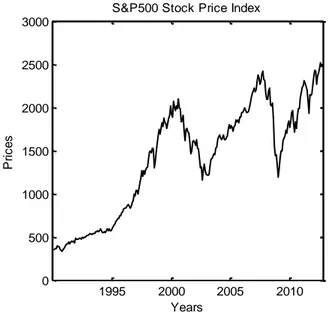
To illustrate our approach, we use monthly U.S. financial data for the period January 1990-November 2012, the sample consisting therefore of 275 monthly data. We begin our analysis including only one risky asset that, combined with the risk-free one, constitute the investor optimal portfolio choice.
In our study, the risky asset is the S&P 500 Index, and the risk-free asset is a short-term debt instrument.
The S&P 500 is the most widely accepted barometer of the market. This value weighted index was firstly compiled in 1957 when it included 500 of the largest industrial, rail, and utility firms that traded on the New York Stock Exchange. It soon became the standard against which the performance of institutions and money managers investing in large U.S. stocks was compared. It now includes 500 large-cap stocks, which together represent about 75% of the total U.S. equities market. The
25 S&P 500 thus provide a convenient way to examine the behavior of stock returns. Returns on the index were computed assuming continuous compounding, from the monthly total return time series downloaded from Datastream.
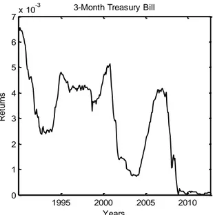
The risk-free asset used in the analysis is the 3-month Treasury Bill, downloaded from FRED (Federal Reserve Economic Data) a database of the of the Federal Reserve Bank of St. Luis. The available data are annualized, therefore we divided the annualized rates by 12 in order to get the monthly rates of return.
2.3.1 Preliminary analysis
Equity index’s total return time series is non-stationary and it has frequent changes in mean, as it is displayed in Figure 2.1.
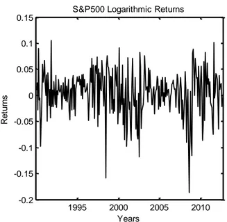
Returns instead exhibit more attractive properties, that is the reason why we use returns in place of prices series throughout our work. Continuous compounded returns are computed according to equation (1.3), starting from the total return series of the stock index. We now make a brief analysis of these returns properties. The returns considered here are stationary, and the autocorrelation function confirms that.
1995 2000 2005 2010 0 500 1000 1500 2000 2500 3000 Years P ri c e s
S&P500 Stock Price Index
26
Moreover analyzing the empirical autocorrelation function we can see that returns are uncorrelated. They have a positive mean of 0.0070, that is significant since the t-statistic (obtained dividing the returns’ mean by its standard error) , is equal to 2.6945 , which is greater than the critical value 1.96.
S&P500 Logarithmic Returns
Mean 0.007082 St. Error 0.002628
Minimum -0.183863 Variance 0.001900
Maximum 0.108277 St. Dev 0.043587
1° Quartile -0.017341 Skewnees -0.773007 3° Quartile 0.035467 Kurtosis Excess 1.579464
1995 2000 2005 2010 -0.2 -0.15 -0.1 -0.05 0 0.05 0.1 0.15 Years R e tu rn s
S&P500 Logarithmic Returns
Figure 2.2: S&P 500 Continuously Compounded Returns over the period 1990-2012
Table 2.1: Main descriptive statistics of S&P 500 Continuously Compounded Returns over the period 1990-2012.
27 When returns are calculated assuming continuous compounding they are hypothesized to have a Normal distribution. This hypothesis hold true for multiperiod returns as well, since they are simply the sum of the continuously compounded one-period returns involved. The assumptions of normality, attributed to the assets’ returns, has a fundamental role in the construction of the model, however there are empirical reasons to believe that it does not represent an adequate description of the returns’ generator process. We now test for the normality of our sample.
There are several test statistics that can be used in order to verify the normality of the returns series. The simplest ones are based on the properties of the indexes of skewness and kurtosis. Indeed under normality assumption S xˆ( )andK xˆ ( ) 3 are distributed asymptotically as normal with zero mean and variance 6 / Tand 24 / T, respectively. These asymptotic properties can be used to test the normality of asset returns. Given our asset series, the skewness and excess of kurtosis of returns can be verified throughout the use of marginal tests respectively based on S and K. Jarque and Bera (1987) combine the two tests and use the test statistic
2 2 ˆ ˆ 3 , 6 / 24 / S K JB T T
which is asymptotically distributed as a chi-squared random variable with 2 degrees of freedom, to test for the normality of asset return series.
0 5 10 15 20 -0.5 0 0.5 1 Lag A C F
Sample Autocorrelation Function
0 5 10 15 20 -0.5 0 0.5 1 Lag P A C F
Sample Partial Autocorrelation Function
28
Another statistic used in order to test for the hypothesis of normality, when the mean and variance are not specified, is the Lilliefors one. Initially the empirical mean and variance are estimated from the available data, then the maximum discrepancy between the empirical distribution function and the cumulative distribution function of the normal distribution, with the estimated mean and variance, is found . Finally the obtained statistic value is compared with the critical values of the Lilliefors distribution in order to assess whether the maximum discrepancy is large enough to be statistically significant , thus requiring rejection of the null hypothesis.
Normality Test Jarque-Bera 0.001 Lilliefors 0.023
Our results reject the null hypothesis of normal returns for a significance level of 0.05. A confirmation of what has been said, the normal probability plot in Figure 2.5 shows a departure of sample quantiles from the theoretical ones of the normal distribution, in particular on the left queue. Moreover, the empirical density function of the returns series in Figure 2.4, has a particularly high peak around its mean and exhibits a skewness on the left side and leptokurotsis, sign that extreme returns are more likely to happen compared to a normal distribution.
-0.2 -0.1 0 0.1 0.2 0 2 4 6 8 10 12
Normal Density Plot
Table 2.2: Normality tests’ P-values for the returns series.
Figure 2.4: Empirical density function of the S&P 500 returns series and normal probability density function evaluated by using the sample mean and standard deviation.