Classification of Clausocalanus Furcatus mobility

(1)

Alma Mater Studiorum ⋅ Università di Bologna

Scuola di Scienze

Dipartimento di Fisica e Astronomia Corso di Laurea in Fisica

Classification of Clausocalanus

Furcatus Mobility

Relatore:

Prof. Armando Bazzani

Correlatore:

Dott. Nico Curti

Presentata da:

Diego Cardinali

(2)

A mio nonno Marino Sit tibi terra levis

06/06/1942 10/10/2020

(3)

Abstract

The purpose of this work is the classification of the main properties of the mobility of the species Clausucalanus furcatus. This classification is then used to propose a model for the motion of the specimens divided in a fast regime a slow regime, with an ulterior distinc-tion between environments in which food is present or absent. For the slow regime the specimens appear to move mostly upwards or downwards for short time periods, whereas the motion in the fast regime is compatible with the Lévy flight foraging hypothesis. In environments where food is scarce C. Furcatus also appears to adopt some energy con-servation strategies, increasing the time between more expensive activities such as long jumps.

Sommario

Scopo di questo lavoro è la classificazione delle principali proprietà di mobilità della specie

Clausocalanus Furcatus. Questa classificazione è poi utilizzata per proporre un modello

per il moto degli esemplari diviso in un regime veloce e un regime lento, con ulteriore distinzione sulla presenza o meno di cibo nell’ambiente. Nel regime lento gli individui tendono a muoversi di moto ascendente o discendente per brevi periodi di tempo, mentre il regime veloce appare compatibile con l’ipotesi di foraggiamento tramite processi di Lévy. In ambienti privi di cibo emerge anche l’adozione da parte di C. Furcatus di strategie di risparmio energetico, dilatando i tempi tra attività più dispendiose quali spostamenti particolarmente lunghi.

(4)

Introduction

The purpose of this work is the classification of the main properties of the mobility of Clausocalanus furcatus, a species of copepods that can be found in various marine locations including the gulf of Naples (IT), where the samples analysed in this work have been collected.

The main goal of this thesis is to propose a simplified model for the motion of the specimens of C. furcatus based mainly on two factors: velocity of the individual and presence (or absence) of food in the environment. Regarding the velocity, the motion of the creatures has been divided in fast and slow regime based on specific thresholds that emerged during the analysis and that seem to depend on whether or not food is present. The second factor, other than dictating the velocity threshold, also seems to be related to the behaviour of the creatures concerning spatial exploration.

This work is divided into chapters, what follows now is a brief overview of the content of each one.

The first chapter contains a brief introduction to some concepts of probability, mostly focused on power-law probability density functions, and stochastic processes. Afterwards Markov processes are introduced and then, more specifically, diffusion processes. These are determinant to introduce the main stochastic process used in the proposed model, the Lévy flight. After presenting these objects, the Lévy flight foraging hypothesis is quickly introduced. The chapter concludes with the concept of hazard function from survival analysis, where a physical interpretation is given for the hazard function of a power-law probability density function.

The second chapter contains an overview of the concept of Frenet-Serret frame for a 3-dimensional curve, then the calculations for the curvature and torsion of a helix, that are used to test the accuracy and behaviour of a portion of the code subsequently used in the analysis.

The third chapter follows the steps of the analysis performed, first by examining the velocities and determining threshold values to distinguish between motion regimes, then by exploring various properties of the motion. After the division, a test is conducted to check whether or not the mean behaviour of the individuals matches that of the whole set of data, followed by a classification of the durations and lengths of the trajectories. The final part of the chapter contains a more detailed overview of the space exploration properties for the trajectories by examining the curvature and torsion probability density functions.

The fourth and final chapter contains a summarisation of all the previous results, which are combined to formulate the proposed model for the motion of C. Furcatus.

To conclude, a small appendix contains an overview of the Kolmogorov-Smirnov test, which is used throughout this thesis to check the confidence level of all curve fits on the

(6)

probability density functions.

All the code used for the analysis in this thesis is free and open source software, and it is available at [Car20a], [Car20b] under the terms of The Unlicense.

(7)

1. Elements of Probability and

Stat-istics

1.1 Probability

Let 𝒫 (𝑥) be a probability density function (𝑃 𝐷𝐹) for a random variable 𝜉, then its associated cumulative distribution (𝐶𝐷𝐹) is defined as

𝑃 (𝑥) ≡ 𝑃 (𝜉 ≤ 𝑥)def= ∫

𝑥 −∞

𝒫 (𝑦)d𝑦 . (1.1)

By definition of 𝑃 𝐷𝐹 it follows immediately that 𝑃 (+∞) = lim

𝑥→+∞∫

𝑥 −∞

𝒫 (𝑦)d𝑦 = 1 , (1.2)

so another useful definition is that of the complementary 𝐶𝐷𝐹 1

𝑃 (𝑥)def= 1 − 𝑃 (𝑥) = ∫

+∞ 𝑥

𝒫 (𝑦)d𝑦 . (1.3)

In the Data Analysis chapter a commonly used 𝑃 𝐷𝐹 will be the power law

𝒫 (𝑥) = 𝐶 (𝑥 − 𝑥₀)𝛼 , (1.4)

with 𝐶, 𝛼, 𝑥0 ∈ ℝ such that the normalisation condition is satisfied over the dominion.

Whenever these distributions will be applied they will represent the actual 𝑃 𝐷𝐹 only for values of 𝑥 such that 𝑥 − 𝑥0 > 0, so the fact that the base is positive also implies

that for all the cases in this thesis it will always be assumed 𝛼 < 0, otherwise the 𝑃 𝐷𝐹 would diverge. Given these considerations, it is useful to rewrite (1.4) as

𝒫 (𝑥) = {𝐶 (𝑥 − 𝑥0)

𝛼

𝑥 ≥ 𝑥₀

0 𝑥 < 𝑥₀ . (1.5)

The 𝐶𝐷𝐹 for a 𝑃 𝐷𝐹 in the form (1.5) is found by solving the integral (1.1) 𝑃 (𝑥) = ∫ 𝑥 −∞ 𝐶 (𝑦 − 𝑥₀)𝛼d𝑦 = ∫ 𝑥 𝑥0 𝐶 (𝑦 − 𝑥₀)𝛼d𝑦 = = 𝛼≠−1[ 𝐶 𝛼 + 1(𝑦 − 𝑥0) 𝛼+1_]𝑥 𝑥0 = 𝐶 𝛼 + 1(𝑥 − 𝑥0) 𝛼+1 _. (1.6)

(8)

1.2 Stochastic Processes and Markov Processes

A stochastic system is a system that evolves probabilistically in time or, more precisely, any system in which there exists a time-dependent random variable 𝜉 (𝑡), of which various values 𝑥𝑖 can be measured at times 𝑡𝑖. In any stochastic system one can always assume

the existence of a set of 𝑃 𝐷𝐹s called joint probability densities

𝒫 (𝑥₁, 𝑡₁; 𝑥₂, 𝑡₂; ...) . (1.7)

Given 𝒫, it is also possible to introduce a conditional joint probability of a series of events (𝑥₁, 𝑡₁; 𝑥₂, 𝑡₂; ...) provided that other events (𝑦₁, 𝜏₁; 𝑦₂, 𝜏₂; ...) have already happened. This conditional 𝑃 𝐷𝐹 is indicated as

𝒫 (𝑥₁, 𝑡₁; 𝑥₂, 𝑡₂; ...|𝑦₁, 𝜏₁; 𝑦₂, 𝜏₂; ...)def= 𝒫 (𝑥1, 𝑡1; 𝑥2, 𝑡2; ...; 𝑦1, 𝜏1; 𝑦2, 𝜏2; ...)

𝒫 (𝑦₁, 𝜏₁; 𝑦₂, 𝜏₂; ...) , (1.8) where times are usually considered ordered decreasingly (even though these probability densities are independent of the order of times), giving

𝑡₁ ≥ 𝑡₂ ≥ ... ≥ 𝜏₁ ≥ 𝜏₂ ≥ ... . (1.9)

To define a stochastic process it is necessary to know at least all joint probabilities (1.7) [Gar09], and the process will be called separable if this is enough to define it. There are four kinds of such processes: completely independent, Bernoulli trials, martingales and Markov processes. For this thesis only the last ones are relevant, and so will be expanded upon.

In a Markov Process the knowledge of the present determines the future via a relation called Markov assumption. If times are ordered as in (1.9), the Markov assumption requires the conditional probability to be entirely determined by the knowledge of the most recent condition, i.e.

𝒫 (𝑥₁, 𝑡₁; 𝑥₂, 𝑡₂; ...|𝑦₁, 𝜏₁; 𝑦₂, 𝜏₂; ...) = 𝒫 (𝑥₁, 𝑡₁; 𝑥₂, 𝑡₂; ...|𝑦₁, 𝜏₁) . (1.10) This assumption means that everything can be defined in terms of the simple conditional probabilities 𝒫 (𝑥1, 𝑡1|𝑦1, 𝜏1). As an example, given

𝒫 (𝑥₁, 𝑡₁; 𝑥₂, 𝑡₂|𝑦₁, 𝜏₁) = 𝒫 (𝑥₁, 𝑡₁|𝑥₂, 𝑡₂; 𝑦₁, 𝜏₁) 𝒫 (𝑥₂, 𝑡₂|𝑦₁, 𝜏₁) , then from the Markov assumption it follows

𝒫 (𝑥₁, 𝑡₁; 𝑥₂, 𝑡₂; 𝑦₁, 𝜏₁) = 𝒫 (𝑥₁, 𝑡₁|𝑥₂, 𝑡₂) 𝒫 (𝑥₂, 𝑡₂|𝑦₁, 𝜏₁) ,

where each 𝒫 is now fully characterised based only on the immediately preceding event. For the sake of completeness, this example can be generalised for an arbitrary joint probability as [Gar09] 𝒫 (𝑥₁, 𝑡₁; ...; 𝑥_𝑛, 𝑡_𝑛) = 𝒫 (𝑥_𝑛, 𝑡_𝑛) 𝑛−1 ∏ 𝑖=1 𝒫 (𝑥_𝑖, 𝑡_𝑖|𝑥_𝑖+1, 𝑡_𝑖+1) . (1.11)

(9)

1.3 Diffusion Processes

A diffusion process is a particular kind of Markov process widely used to model the movement of objects of any kind, from particles to small animals. Any diffusion process can be divided into two phases: in the first one the objects are in a non-equilibrium environment, and thus there is a concentration gradient that drives the process; when the concentration of the particles drifting is uniform the gradient becomes zero and thus the particles do not drift anymore as an ensemble (but they still move randomly in all directions). Diffusion processes are usually modelled via partial differential equations, as these tend to be easy to solve numerically with a good degree of precision. Let 𝜉 be a random variable associated to a continuous-state, continuous-time Markov process Ξ (𝑡), that is, a process in which both 𝜉 and 𝑡 are continuous. Ξ (𝑡) is also called the sample path of 𝜉, i. e. the time progression of the samples drawn from 𝜉. The conditional 𝐶𝐷𝐹 for the process is

𝑃 (𝑥, 𝑡|𝑦, 𝜏) = 𝑃 (Ξ (𝑡) ≤ 𝑥|Ξ (𝜏) = 𝑦) . (1.12) if the derivative of 𝑃 with respect to 𝑥 exists, it is called the transition density function of the process and its expression is

𝒫 (𝑥, 𝑡|𝑦, 𝜏) = 𝜕_𝑥𝑃 (𝑥, 𝑡|𝑦, 𝜏) . (1.13)

In order for Ξ to be considered a diffusion process the required conditions are: • continuity of 𝒫, which implies continuity of Ξ [Ibe13];

• the mean ⟨⋅⟩ of Ξ is related to 𝒫 in the form

lim Δ𝑡→0 ⟨Ξ (𝑡 + Δ𝑡) − Ξ (𝑡) |Ξ (𝑡) = 𝑦⟩ Δ𝑡 = 1 Δ𝑡 ∫_ℝ(𝑥 − 𝑦) 𝜕𝑥𝒫 (𝑥, 𝑡 + Δ𝑡|𝑦, 𝑡)d𝑥 def = 𝑎 (𝑦, 𝑡) , (1.14) where 𝑎 is known as the instantaneous drift of Ξ;

• the variance of Ξ is related to 𝒫 in the form

lim Δ𝑡→0 ⟨[Ξ (𝑡 + Δ𝑡) − Ξ (𝑡)]2|Ξ (𝑡) = 𝑦⟩ Δ𝑡 = 1 Δ𝑡∫_ℝ𝑛 (𝑥 − 𝑦)2𝜕_𝑥𝒫 (𝑥, 𝑡 + Δ𝑡|𝑦, 𝑡)d𝑥 = 𝑏 (𝑦, 𝑡) , (1.15) where 𝑏 is known as the instantaneous variance of Ξ.

(10)

If Δ𝑡 is discrete, let 𝑝 be the probability that Ξ moves of Δ𝑥 after a time increase of Δ𝑡 and 𝑞 = 1 − 𝑝 the probability that it moves of −Δ𝑥. If 𝑝 − 𝑞 tends to 0 as Δ𝑡 and Δ𝑥 tend to 0 it is possible to introduce the coefficients

𝜇def= lim Δ𝑡,Δ𝑥→0 (𝑝 − 𝑞) Δ𝑥 Δ𝑡 , (1.16) 𝒟def= lim Δ𝑡,Δ𝑥→0 (Δ𝑥)2 2Δ𝑡 . (1.17)

If 𝜇 and 𝒟 are constants the diffusion process is described by the Fokker-Planck equation 𝜕_𝑡𝒫 (𝑥, 𝑡|𝑥₀, 𝑡₀) = −𝜇𝜕_𝑥𝒫 (𝑥, 𝑡|𝑥₀, 𝑡₀) + 𝒟𝜕2

𝑥𝒫 (𝑥, 𝑡|𝑥0, 𝑡0) . (1.18)

A characteristic quantity for diffusion processes is the mean square displacement (𝑀𝑆𝐷). Let there be a system with 𝑛 particles identified by the index 𝑖, each with starting position 𝑥_0𝑖 and a position 𝑥_𝑖(𝑡) at time 𝑡, then the 𝑀𝑆𝐷 is

𝑋2_(𝑡)def₌ 1 𝑛 𝑛 ∑ 𝑖=1 ⟨[𝑥_𝑖(𝑡) − 𝑥_0𝑖]2⟩ . (1.19)

This quantity is closely related to the diffusion coefficient 𝒟 by the power law [BH00]

𝑋2 _{∝ 𝐷𝑡}𝛾 _(1.20)

with 𝛾 ∈ ℝ. The value of 𝛾 is determinant for the type of diffusion. If 𝛾 = 1 the 𝑀𝑆𝐷 is proportional to the diffusion coefficient the process is called standard (or Fickian) diffusion, and it obeys Fick’s law, otherwise it is called anomalous diffusion, and in particular sub-diffusion if 𝛾 < 1, super-diffusion if 𝛾 > 1 [Kla+90].

The case for 𝛾 = 1 is the standard Brownian Motion, as it is proven in [Zan], meaning that the 𝑀𝑆𝐷 is directly proportional to the diffusion coefficient, so space exploration grows linearly in time.

In the case 𝛾 < 1 the underlying probability density for a particle to be at a position 𝑟 at time 𝑡 is non-Gaussian. This regime is usually obtained by adding physical or temporal constraints to the system, limiting the freedom of movement for the particles. The regime 𝛾 > 1 on the other hand is also often called enhanced transportation, and it will be expanded upon in the next section of this chapter.

1.4 Lévy Flights and the Lévy Flight Foraging Hypothesis

Lévy Flights are processes characterised by a 𝑃 𝐷𝐹 for the length of the step in the form

(11)

so that their sample path is described by clusters of random points interjected by in-frequent longer jumps, the flights that give the phenomenon its name. The mean and the variance of 𝒫 diverge along with the 𝑀𝑆𝐷 [Kla+90]. This last quantity in par-ticular satisfies Eq. (1.20) for 𝛾 > 1, meaning that Lévy flights are topical examples of super-diffusive processes.

Because of the aforementioned non-convergence problems, Lévy Flights are often trun-cated when applied to real-life scenarios, using a 𝑃 𝐷𝐹 in the form

{𝒫 (𝑥) ∝ 𝑥

𝛼 _𝑥

0 < 𝑥 ≤ 𝑥 ,

0 otherwise . (1.22)

In this case 𝑥 takes the name of cutoff parameter and ensures that the previously di-vergent parameters now converge to a finite value. In this thesis all Lévy flights will be automatically truncated by programmatically choosing as cutoff parameter a value after which the noise on the data becomes too significant. The value of 𝑥0 is usually 0, but

in this work it is necessary to introduce it as not all distributions immediately present a Lévy flight-like fall, so this parameter is used to start fitting when the power-law regime begins.

While Lévy flights have many applications, the one that will be explored in this work is that of the Lévy Flight foraging hypothesis; formulated first in 1999 by Viswanathan et al. in [Vis+99], it can be formally stated as follows:

“Since Lévy flights (actually, truncated Lévy flights) optimize random searches, biological organisms must have therefore evolved to exploit Lévy flights.”

[Rap+09]

The original work from 1999 stated that, under the assumptions of randomly distributed revisitable foraging sites, if Markov assumption (i. e. absence of memory) also holds, the optimal strategy for visiting as many sites as possible is that of an inverse square power-law.

This hypothesis has been heavily debated over the years, finding various confirmations, but also having many results overturned. A recent analysis [Hum+12] found strong evid-ence for a truncated Lévy flight driven exploration in wandering albatross (Diomedea

ex-ulans) and black-browed albatross (Thalassarche melanophrys) when information about

the environment is not complete, i. e. the animal can not rely on visual, auditory or olfactory clues to identify the prey from afar or is not familiar with the environment. Since the purpose of this work is to investigate the behaviour of specimens of Clausocalanus

Furcatus both in conditions where food is present and where it is not, a main driving

idea of this investigation will be that the individuals tend to explore the space in a Lévy flight-like distribution when going over a certain threshold velocity, as to verify whether or not this hypothesis could apply to the motion of this species.

(12)

1.5 Hazard Functions

Later in this work a key part of the behavioural analysis performed will be focused on characterising the duration of various tracks, so it is relevant to introduce an im-portant concept of survival analysis: the hazard function. Under the hypothesis of the Markov assumption for the time evolution of the system, the complementary 𝐶𝐷𝐹 sat-isfies [GBR15]

𝑃 (𝑡 + Δ𝑡) = [1 − λ (𝑡) Δ𝑡] 𝑃 (𝑡) + 𝑜 (Δ𝑡) , (1.23) where λ is the hazard function, i. e. the event rate at 𝑡 conditional on a duration of at least 𝑡. In the continuous case, for the limit of Δ𝑡 that goes to 0, from this relation it is possible to find an expression for λ (𝑡) by simple algebraic manipulation of (1.23):

𝑃 (𝑡 + Δ𝑡) − 𝑜 (Δ𝑡) 𝑃 (𝑡) = 1 − λ (𝑡) Δ𝑡 ⟹1 − 𝑃 (𝑡 + Δ𝑡) − 𝑜 (Δ𝑡) 𝑃 (𝑡) = λ (𝑡) Δ𝑡 ⟹ 1 𝑃 (𝑡) 𝑃 (𝑡) − 𝑃 (𝑡 + Δ𝑡) − 𝑜 (Δ𝑡) Δ𝑡 = λ (𝑡) ,

and by taking the limit it follows that

λ(𝑡) = lim Δ𝑡→0 1 𝑃 (𝑡) 𝑃 (𝑡) − 𝑃 (𝑡 + Δ𝑡) − 𝑜 (Δ𝑡) Δ𝑡 ⟹λ (𝑡) = −d𝑡𝑃 (𝑡) 𝑃 (𝑡) . An immediate consequence of 1.3 is d𝑡𝑃 (𝑡) =d𝑡(1 − 𝑃 (𝑡)) =

so the final expression for the hazard function is

λ(𝑡) = 𝒫 (𝑡) 𝑃 (𝑡) = 𝒫 (𝑡) 1 − ∫𝑡 −∞𝒫 (𝜏)d𝜏 . (1.24)

Via direct substitution of the Eqs. (1.5, 1.6) in the newfound expression, it is possible to find the theoretical expression for the hazard function of the power law probability density function

λ(𝑡) = 𝐶 (𝑡 − 𝑡0)

𝛼

(13)

2

4

6

8

10 t

0.0

0.5

1.0

1.5

t

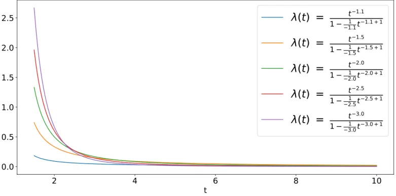
3.0 + 1

Figure 1.1: Various hazard functions for 𝑃 𝐷𝐹s in the form (1.4) with 𝐶 = 1, 𝑡0 = 1.5

and a cutoff parameter 𝑡 = 10. These values for 𝛼 are all in the interval −3 ≤ 𝛼 < −1 to remain within the boundaries of the Lévy flight phenomena. The minimum value chosen for the exponent was 𝛼 = −1.1 as 𝛼 = −1 would cancel the denominator.

In the case of a Lévy flight distribution (−3 ≤ 𝛼 < −1) some notable examples for the hazard function can be seen in Fig. 1.1 (case 𝐶 = 1, 𝑡0 = 1.5, 𝑡 = 10). These

allow to give a reasonable physical interpretation to the hazard function of a power-law probability density function. If the 𝑃 𝐷𝐹 is interpreted as the distribution of durations of a trip for a particle, the hazard function represents the conditional probability density function that a trip will end at a certain time 𝑡 + Δ𝑡 provided that it lasted 𝑡.

As it can be seen in the figure, the function is strictly decreasing, meaning that for short trips it is much more likely for the particle to stop. As time passes and the trip becomes longer however, the probability to stop quickly decreases, until the cutoff parameter 𝑡 is reached. The purpose of the cutoff parameter is to make it impossible for the particle to travel for an infinite amount of time, since that would clearly not be physical.

This incremental incentive to make the trip longer suggest a sort of intentionality, i. e. when a trip lasts longer it means that the traveller has a specific intent of reaching a further point, so in the case of an animal it may be interpreted as a deliberate choice to search for some points of interest (food, a mate, a shelter...).

(14)

2. Frenet-Serret Curve Theory

2.1 Frenet-Serret Apparatus

To properly introduce a Frenet-Serret apparatus for a point it is first necessary to char-acterise its motion. Motion can be defined as a continuous succession of events described by a differentiable application

⃗

𝑟 ∶ ℝ ⟶ ℝ3

𝑡 ⟼ ⃗𝑟 (𝑡), (2.1)

where 𝑡 is usually identified with the time and ⃗𝑟 is often referred to as motion law. The plot of ⃗𝑟 in ℝ3 _{is called trajectory or orbit. Given two points ⃗𝑟}

1 = (𝑥, 𝑦, 𝑧) and

⃗

𝑟₂ = (𝑥 +d𝑥, 𝑦 + d𝑦, 𝑧 + d𝑧), the length of ⃗𝑟₂ − ⃗𝑟₁ constitutes the arc length of an infinitesimal portion of the curve

d𝑠2 ₌_d𝑥2₊_d𝑦2₊_d𝑧2 _, _(2.2)

and by introducing the velocity ⃗𝑣 as the derivative with respect to 𝑡 of the trajectory, the arc length can be expressed as

d𝑠 = √d𝑥2₊d𝑦2₊d𝑧2 _{= √(}d

𝑡𝑥)2+ (d𝑡𝑦)2+ (d𝑡𝑧)2d𝑡 = ‖ ⃗𝑣(𝑡)‖ d𝑡 . (2.3)

The kinematic component of the motion can be separated from the purely geometrical one by rewriting (2.1) as

⃗

𝑟 = ⃗𝑟 (𝑠) , 𝑠 = 𝑠 (𝑡) . (2.4)

The first equation now describes only the trajectory, so it can be used to introduce three unitary orthogonal vectors which constitute the so called Frenet-Serret frame [Tur99]

⃗ 𝑇 (𝑠) def=d_𝑠𝑟 (𝑠) ,⃗ (2.5) ⃗ 𝑁 (𝑠)def= 1 ∥𝑑_𝑠𝑇 ∥⃗ d𝑠 ⃗ 𝑇 (𝑠) = 1 𝜅d𝑠𝑇 (𝑠) ,⃗ (2.6) ⃗ 𝐵 (𝑠) def= ⃗𝑇 (𝑠) ×𝑁 (𝑠) .⃗ (2.7)

The quantity 𝜅 is called curvature and it is the inverse of the curvature radius, i. e. the radius of the circle arc that best approximates the curve at that particular point. It follows that if 𝜅 tends to 0, the curve tends to a straight line. The three vectors of the

(15)

frame are called respectively tangent, normal and binormal. By using these vectors it is possible to build what is called a Frenet-Serret apparatus via a set of equations that completely characterise the curve at any point in space. These equations are

d_𝑠_{𝑇 = 𝜅 ⃗}⃗ _{𝑁 ,} _(2.8)

d𝑠𝑁 = −𝜅 ⃗⃗ 𝑇 + 𝜏 ⃗𝐵 , (2.9)

d𝑠𝐵 = −𝜏 ⃗⃗ 𝑁 , (2.10)

where the quantity 𝜏 is called torsion and is defied via the relation (2.10). The torsion describes the characteristic velocity at which the curve is leaving its osculating plane, that is defined as the plane orthogonal to the binormal vector. The preceding equations are called Frenet-Serret equations and the set of ⃗𝑇, ⃗𝑁, ⃗𝐵, 𝜅 and 𝜏 is called the Frenet-Serret apparatus.

2.2 Implementation and Testing of the Frenet-Serret Apparatus

The analysis of the 3D trajectories presented in the Data Analysis chapter was performed via a code that can be found free of license at [Car20b]. The computational part was written in C++, while the graphical part was implemented in Python. In order to test the accuracy of the numerical methods used, a test was conducted on a helix of equations

⎧ { ⎨ { ⎩ 𝑥 = 𝑅 cos (𝑡) 𝑦 = 𝑅 sin (𝑡) 𝑧 = 𝐴𝑡 , (2.11)

with a radius 𝑅 = 3.0 and a pitch 2𝜋𝐴 = 2𝜋 ⋅ 0.3. To check if the behaviour of the code is correct the equation must be firstly parametrised with 𝑠 such that the velocity becomes unitary. This can be achieved by using

𝑠 (𝑡) = √𝑅2_{+ 𝐴}2 _{𝑡 ,} (2.12) so that ⃗ 𝑟 (𝑠) = (𝑅 cos (√ 𝑠 𝑅2_{+ 𝐴}2) , 𝑅 sin ( 𝑠 √ 𝑅2_{+ 𝐴}2) , 𝐴𝑠 √ 𝑅2 _{+ 𝐴}2) . (2.13)

The tangent can be obtained by direct derivation of the motion law as

⃗ 𝑇 =d_𝑠𝑟 =⃗ √ 1 𝑅2_{+ 𝐴}2 (−𝑅 sin ( 𝑠 √ 𝑅2_{+ 𝐴}2) , 𝑅 cos ( 𝑠 √ 𝑅2_{+ 𝐴}2) , 𝐴 √ 𝑅2_{+ 𝐴}2) ,

and its norm is coherently

‖d𝑠𝑟‖ =⃗

1 √

𝑅2_{+ 𝐴}2√𝑅

(16)

The curvature and the normal vector immediately follow as d𝑠𝑇 = 𝜅 ⃗⃗ 𝑁 = 1 𝑅2 _{+ 𝐴}2 (−𝑅 cos ( 𝑠 √ 𝑅2_{+ 𝐴}2) , −𝑅 sin ( 𝑠 √ 𝑅2_{+ 𝐴}2) , 0) , (2.14) 𝜅 = ∥d_𝑠𝑇 ∥ =⃗ 𝑅 𝑅2_{+ 𝐴}2 , (2.15)

proving that for a helix the curvature is constant. The binormal vector is obtained from the cross product of ⃗𝑇 and ⃗𝑁 as

⃗ 𝐵 = √ 1 𝑅2_{+ 𝐴}2 (𝐴 sin ( 𝑠 √ 𝑅2_{+ 𝐴}2) , −𝐴 cos ( 𝑠 √ 𝑅2_{+ 𝐴}2) , 𝑅) , (2.16)

from which the torsion d𝑠𝐵 = −𝜏 ⃗⃗ 𝑁 = 𝐴 𝑅2_{+ 𝐴}2(cos ( 𝑠 √ 𝑅2_{+ 𝐴}2) , sin ( 𝑠 √ 𝑅2_{+ 𝐴}2) , 0)) ⟹ 𝜏 = 𝐴 𝑅2_{+ 𝐴}2 . (2.17)

The last relation found shows that the torsion is also constant for a helix. Using the parameters for the test one finds

𝜅 = 0.3300 , 𝜏 = 0.0330 .

Two numeric tests were conducted with different parametrisations. The first aimed at studying an almost continuous case, where the parameter 𝑡 ranged from 0 to 6𝜋 with an increment of 0.0002𝜋 every step, for a total of 30000 steps. In this case the values obtained (after being divided by the increment to correctly rescale 𝑡) are

𝜅 = 0.33003300 , 𝜏 = 0.03300330 ,

which are perfectly coherent with the theoretical one up to the eighth decimal place. For the second test the parameters used were more resembling of common values found in the actual data, with a chosen velocity of 101_{, and the time ranging from 0 to 10 with}

an increment of 0.0666667, for a total of 150 steps. This time the values are

𝜅 = 0.32997114 , 𝜏 = 0.03300304 ,

and as expected, these are less precise, but still resemble the theoretical data with a good degree of precision. The helices obtained with the program using these parameters are reported in Fig. 2.1. The results are as expected, with the correct positioning of all unitary vectors on the curve.

(17)

X 4 ₃ 2 ₁ 0 ₁ 2 ₃ 4 Y 4 3 2 1 0 1 2 3 4 Z 0 1 2 3 4 5 6

Helix

Tangent

Normal

Binormal

X 4 ₃ 2 ₁ 0 ₁ 2 ₃ 4 Y 4 3 2 1 0 1 2 3 4 Z 0 1 2 3 4 5 6

Helix

Tangent

Normal

Binormal

Figure 2.1: Test helices obtained via the code at [Car20b]. Both helices have a radius 𝑅 = 3 and a pitch 2𝜋𝐴 = 2𝜋 ⋅ 0.3 so the curvature is 𝜅 = 0.3300 and the torsion is 𝜏 = 0.0330. The helices have different parametrisations. The top one has the parameter 𝑡 ∈ [0, 6𝜋] with an increment of 0.0002𝜋, for a total of 30000 steps, the bottom one has 𝑡 ∈ [0, 10] with an increment of 0.0666667, for a total of 150 steps. In order to maintain legibility only one set of unitary vectors every 𝑘 points is drawn, for the top plot 𝑘 = 800, for the bottom one 𝑘 = 8. The red unitary vector is the tangent, the green one is the normal and the black one is the binormal.

(18)

3. Data Analysis

3.1 Structure of Data

The data analysed in this work consists of four experiments [Pas+18], which will be referred to as E1, E2, E3, E4. Numerous zooplankton samples were collected from the Gulf of Naples in 2008 (for E1, E2) and 2009 (for E3, E4). Healthy adult females of the species Clausocalanus furcatus were selected among these and isolated in two groups of 30 and 37 individuals, that were consequently recorded in a 1ℓ aquarium for one hour either in the presence of food or without it. E1 and E3 were recorded in the presence of small food particles, with a density of 𝜌𝑓1 = 5 ⋅ 105 units/ℓ and 𝜌𝑓3 = 5 ⋅ 106 units/ℓ

respectively, whereas E2 and E4 were conducted in the absence of food using filtered sea water.

A series of coordinates in the 2-dimensional space were acquired via an automated system of cameras with a spatial resolution of 78 𝜇𝑚 at 15 𝑓𝑝𝑠. The system can be seen in Fig. 3.1. The merging of the trajectories in 3-D was performed via a C++ code used to combine the simultaneous 2-D tracks by comparing the common 𝑧 values and discard ghost tracks (non moving objects). All trajectories shorter than 5 𝑠 were discarded. Information about the final 3-D trajectories are given in Tab. 3.1.

An example of a track can be seen in Fig. 3.2. This particular track is a segment of an even longer track from 𝐸3, in which the specimen is moving at a high velocity (𝑣 > 6𝑚𝑚/𝑠) in a convoluted pattern.

Experiment Tracks Average duration (𝑠) Minimum duration (𝑠) Maximum duration (𝑠)

E1 (food) 255 23.9 5 241

E2 (no food) 384 28.9 5 342

E3 (food) 625 24.4 5 278

E4 (no food) 425 35.2 5 277

Table 3.1: Number of tracks, average duration, minimum duration and maximum dur-ation of the four experiments E1, E2, E3, E4. E3 and E4 have significantly more data than E2 and, especially, E1, as not only do the other experiments have more tracks, they also have a higher average duration, meaning more points overall.

(19)

Figure 3.1: An image of the experimental setup taken from [Bia+13]. The labelled components are respectively: a digital camera (A); a telecentric lens (B); an infrared light source (C); a 1 ℓ aquarium containing the samples (D); an empty 8 ℓ aquarium used for protection from external disturbances (E). The sampling rate chosen for the experiments was 15 𝑓𝑝𝑠, the spatial resolution of the cameras was 78 𝜇𝑚.

X

6466

₆₈₇₀

7274

7678

₈₀

Y

25

30

35

40

45 Z

7.5

10.0

12.5

15.0

17.5

20.0

22.5

25.0 Trajectory

Figure 3.2: A long trajectory taken from E3, the loop structures tend to be quite common along with spiralling ones and quick dives both upwards and downwards.

(20)

3.2 Velocities: Fast and Slow Regimes

The first step of the analysis involved the study of the velocities of C. Furcatus specimens. The time-step between two points is 𝑡 = 1/15 𝑠 = 0.06 𝑠, so given two sets coordinates

⃗

𝑥₁, ⃗𝑥₂ ∈ ℝ3, the velocity is simply

⃗

𝑣₁ = 𝑥⃗2− ⃗𝑥1

𝑡 . (3.1)

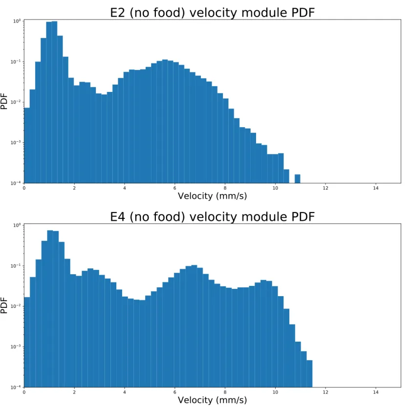
For each experiment the 𝑃 𝐷𝐹 of the velocity modules can be seen in Figs. 3.3 for the two experiments with food and 3.4 for the ones without. For E2 and E4 the distributions have similar structures, both with the largest peak between 1 𝑚𝑚/𝑠 and 2 𝑚𝑚/𝑠 and a smaller peak between 2 𝑚𝑚/𝑠 and 3 𝑚𝑚/𝑠. Both also have another peak between 5 𝑚𝑚/𝑠and 7 𝑚𝑚/𝑠, however the E2 𝑃 𝐷𝐹 lacks a fourth peak, which is instead present in the E4 𝑃 𝐷𝐹 between 9 𝑚𝑚/𝑠 and 10 𝑚𝑚/𝑠. An important part of the analysis is to find whether there is a difference in behaviour as velocity increases, therefore a threshold velocity has been defined to distinguish between fast and slow regime. For E2 and E4 this velocity was chosen at the end of the first peak at 𝑣cut

2,4 = 2.1 𝑚𝑚/𝑠, and all of the

subsequent analysis has been conducted separately between the two regimes to highlight behavioural differences.

The distributions for E1 and E3 showcase more differences, as the E1 𝑃 𝐷𝐹 has two distinct peaks at slow velocities, one between 1 𝑚𝑚/𝑠 and 2 𝑚𝑚/𝑠, the other between 2 𝑚𝑚/𝑠 and 3 𝑚𝑚/𝑠, whereas the E3 𝑃 𝐷𝐹 only manifests the first one. The E1 𝑃 𝐷𝐹 also has a smaller peak between 5 𝑚𝑚/𝑠 and 6 𝑚𝑚/𝑠, and a final and taller peak at 10 𝑚𝑚/𝑠, while the E3 distribution lacks the smaller peak and instead manifests a way larger peak at high velocities between 10 𝑚𝑚/𝑠 and 13 𝑚𝑚/𝑠. This last one is notably lower than the peak at slow velocities, but it also has a longer tail than the one of E1, as the 𝑃 𝐷𝐹 for a velocity of 12 𝑚𝑚/𝑠 is already below 10−3 _{for E1, while it is still}

peaking for E3. These anomalies were further investigated by trying to compute the E1 velocities in two alternative ways to see if this would have helped to reproduce a 𝑃 𝐷𝐹 more similar to that of E3.

The first attempt made was to compute a double step velocity, i. e. given three consecutive points ⃗𝑥1, ⃗𝑥2, ⃗𝑥3 ∈ ℝ3, the velocity was computed skipping ⃗𝑥2 using

⃗

𝑣₁ = 𝑥3⃗ − ⃗𝑥1

2𝑡 , (3.2)

however, as it can be seen in the first graph of Fig. 3.5, this only increased the spacing between the two low velocity peaks with little effect on the width of the fastest peak. The second attempt was made using a running average procedure to smooth the peaks, i. e. given 2𝑁 + 1 consecutive velocities ⃗𝑣−𝑁, ..., ⃗𝑣0, ..., ⃗𝑣𝑁 ∈ ℝ3 the averaged velocity

(21)

was computed as ‖ ⃗𝑣‖𝑎𝑣𝑔₀ = 1 2𝑁 + 1 𝑁 ∑ 𝑖=−𝑁 ‖ ⃗𝑣_𝑖‖ , (3.3)

where ‖ ⃗𝑣‖ is the 3-dimensional euclidean norm of the vector. The second graph in Fig. 3.5 shows the averaged 𝑃 𝐷𝐹 for 𝑁 = 2, and as expected this smoothed the peaks, however without any significant effect on making the overall shape of the distribution look more similar to the E3 one. Several other values for 𝑁 were used, up to 𝑁 = 7, without any significant improvement, therefore this route was abandoned.

Considering the tests made, the threshold velocity for E1 and E3 was chosen at 𝑣cut

1,3 =

6 𝑚𝑚/𝑠, the minimum value between the third and fourth peaks of E1 and far enough from the two peaks of E3. This value was chosen to clearly divide the final peak from the previous ones, and although it is not the minimum for 𝐸3𝑓 it is close enough to it with a low value for the 𝑃 𝐷𝐹.

After identifying the threshold velocities, every track in all the experiments was further divided based on the two motion regimes found. Each track was divided in sub-tracks based on the regime change, with the switch from slow to fast (or vice versa) registered if the animal changed its behaviour for at least 4 frames, i. e. 0.27𝑠. Information about the new trajectories are reported in Tab. 3.2. The fast regime will be referred to with an “f” appended to the experiment name, the slow regime with an “s”.

Experiment Tracks Average duration (𝑠) Minimum duration (𝑠) Maximum duration (𝑠)

E1 (slow, food) 371 8.4 0.27 200.9 E1 (fast, food) 377 7.8 0.27 240.7 E2 (slow, no food) 1716 4.4 0.27 18.9 E2 (fast, no food) 1757 2.0 0.27 24.5 E3 (slow, food) 1664 3.6 0.27 47.5 E3 (fast, food) 1978 4.6 0.27 176.1 E4 (slow, no food) 2750 3.4 0.27 14.0 E4 (fast, no food) 2849 2.0 0.27 120.7

Table 3.2: Number of tracks, average duration, minimum duration and maximum dura-tion of the four experiments after dividing the tracks into the fast and slow regimes. It should be noted that all experiments had at least some tracks which started or ended with 1 to 3 points of a particular regime, hence the actual minimum duration was of only 1 frame despite the division of the track on 4 frames minimum. These cases were however not significant and excluded from the analysis, as they were always less than 3.5% of the total number of tracks.

(22)

0 2 4 6 8 10 12 14

Velocity (mm/s)

E2 (no food) velocity module PDF

0 2 4 6 8 10 12 14

Velocity (mm/s)

104 103 102 101 100

PDF

E4 (no food) velocity module PDF

Figure 3.4: Velocity module logarithmic scale 𝑃 𝐷𝐹s for E2 (top) and E4 (bottom), conducted in the absence of food. The overall shapes of the distributions appear similar for the first part, while the E4 𝑃 𝐷𝐹 shows a final peak that the one from E2 lacks. The threshold velocity to divide in fast and slow regime was chosen at 𝑣cut2,4 = 2.1𝑚𝑚/𝑠

as it is the minimum after the first (and tallest) peak and the only minimum the two distributions have in common.

(24)

0 2 4 6 8 10 12 14

Velocity (mm/s)

104 103 102 101 100

PDF

E1 (food, double step) velocity module PDF

0 2 4 6 8 10 12 14

Velocity (mm/s)

104 103 102 101 100

PDF

E1 (food, running average) velocity module PDF

Figure 3.5: Velocity module logarithmic scale 𝑃 𝐷𝐹s for E1 using alternative ways to compute velocities: a double step velocity (top) and a 2-step running average (bottom). These tests were aimed at reproducing from E1 a 𝑃 𝐷𝐹 more resembling to that of E3 to explain the differences in distributions, but they were not successful, so ultimately the analysis was conducted on the unaltered 𝑃 𝐷𝐹 in Fig. 3.3.

(25)

3.3 Individual Mean Velocities

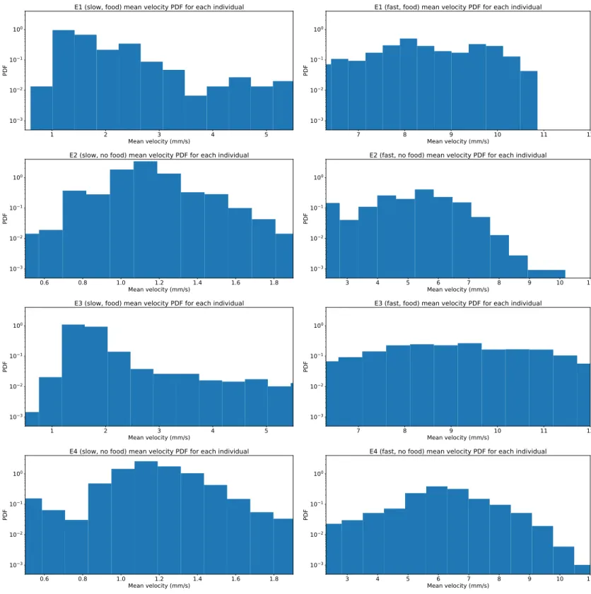
After dividing the data, the first step in the analysis was aimed at understanding if the behaviour of the individual could be used to describe that of the population. In order to do so, the mean velocity of every specimen was computed over each track before finding the 𝑃 𝐷𝐹. Fig. 3.6 shows the 𝑃 𝐷𝐹s found for the mean velocity of each individual, which have been compared to the previous 𝑃 𝐷𝐹s in Figs. 3.3, 3.4.

For the slow regime E1s and E2s show some consistent behaviour with the previous ones as the peaks of the distributions fall in the same intervals, but the height of the peaks have been completely altered. The E1s main peak has increased in height from 0.4 to 1, while the one in E2s rose from 1 to 3. E3s shows a shape similar to that of the previous 𝑃 𝐷𝐹, but the peak has also increased from 0.4 to 1. In E4s the peak has also risen from 0.9 to 3 and there is a non-neglectable portion of specimens that appear to be almost still, while a small portion of velocities localised between 0.6 𝑚𝑚/𝑠 and 0.8 𝑚𝑚/𝑠 appears to be missing. This behaviour is totally lacking in Fig. 3.4. In this regime the hypothesis of using the individuals to identify the sample does not appear to be consistent.

The fast regime shows some notable changes in the structure of the 𝑃 𝐷𝐹s. E1f in this case shows two smaller yet distinct peaks centred at 8 𝑚𝑚/𝑠 and 9.5 𝑚𝑚/𝑠, while it manifested a single peak centred at 10 𝑚𝑚/𝑠 on the original 𝑃 𝐷𝐹. The first peak is also higher than the original peak, from 0.3 to 0.5. E2f retains most of its features but it has its peak increased from 0.1 to 0.6. The large peak from 10 𝑚𝑚/𝑠 to 12 𝑚𝑚/𝑠 in E3f has disappeared and has been replaced by a large peak ranging from 8 𝑚𝑚/𝑠 to 10 𝑚𝑚/𝑠, depriving the 𝑃 𝐷𝐹 of one of its most notable features. E4f loses its smaller peaks around 3 𝑚𝑚/𝑠 and 10 𝑚𝑚/𝑠, while the one centred between 6 𝑚𝑚/𝑠 and 7 𝑚𝑚/𝑠 is retained and has increased in height from about 0.1 to about 0.25. These distributions are completely different to those in Figs. 3.3, 3.4.

These considerations show that the analysis of both regimes can not be carried out on the individuals, but instead requires a large population to be effective and fully characterise the behaviour of the specimens.

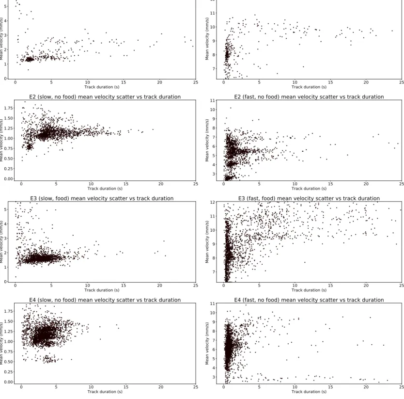
The scatter plots for the mean velocity of each individual as a function of the track length can be seen in Fig. 3.7, and these clearly visualise how E1 has less statistics than the other experiments. An interesting phenomenon is how the clusters of points tend to be horizontally arranged for the slow regime, whereas those from the fast regime tend to be vertically arranged. Slow tracks have therefore less deviation from the mean values of the 𝑃 𝐷𝐹s just discussed, whereas fast tracks are much more diverse and tend to be clustered based on their duration instead of specific velocity values. This kind of clustering near short tracks for the fast regime suggests a motion based on short burst of speed. During these bursts the specimens tend to maintain a constant speed, so various mean values

(26)

are possible for the velocity given the high variability possible. On the contrary, for the slow regime, the tracks tend to be longer and therefore the mean velocity tends to be evened towards specific points, meaning a less erratic motion.

The scatter plots in the fast regime manifest longer tails for various average velocities. The presence of longer jumps is perfectly compatible with a Lévy flight-like motion, and shows that when individuals relocate to a new area they tend to do it at high velocities. The jumps also tend to be more frequent when food is present, as it can be clearly seen by the plot for E3f, where the frequency of longer jumps is much higher than that of E4f. E1f also presents a tail, but its scarcity of trajectories is even more evident in this plot. Even so its tail shows a number of points comparable with that of E2f, so it is not unreasonable to suppose a similar behaviour. In the presence of food the creatures may be incentivised to explore more space, while this costly (in terms of energy) activity may not be encouraged in an environment where food is scarce, paving way for the suggestion of energy preservation strategies. This difference between space exploration, track duration and distance travelled will be the main topic of a following analysis.

(27)

1 2 3 4 5 Mean velocity (mm/s) 103 102 101 100 PDF

E1 (slow, food) mean velocity PDF for each individual

7 8 9 10 11 12 Mean velocity (mm/s) 103 102 101 100 PDF

E1 (fast, food) mean velocity PDF for each individual

0.6 0.8 1.0 1.2 1.4 1.6 1.8 Mean velocity (mm/s) 103 102 101 100 PDF

E2 (slow, no food) mean velocity PDF for each individual

3 4 5 6 7 8 9 10 11 Mean velocity (mm/s) 103 102 101 100 PDF

E2 (fast, no food) mean velocity PDF for each individual

1 2 3 4 5 Mean velocity (mm/s) 103 102 101 100 PDF

E3 (slow, food) mean velocity PDF for each individual

7 8 9 10 11 12 Mean velocity (mm/s) 103 102 101 100 PDF

E3 (fast, food) mean velocity PDF for each individual

0.6 0.8 1.0 1.2 1.4 1.6 1.8 Mean velocity (mm/s) 103 102 101 100 PDF

E4 (slow, no food) mean velocity PDF for each individual

3 4 5 6 7 8 9 10 11 Mean velocity (mm/s) 103 102 101 100 PDF

E4 (fast, no food) mean velocity PDF for each individual

Figure 3.6: Individual mean velocity logarithmic 𝑃 𝐷𝐹s for slow regime (left) and fast regime (right) of all experiments (ordered top to bottom). These distributions describe the mean velocity of a single individual over its entire track, as opposed to those in Figs. 3.3, 3.4 where the 𝑃 𝐷𝐹s are constructed over all velocities for all specimens. By analysing the differences between these 𝑃 𝐷𝐹s and the aforementioned ones it is possible to deduce that studying the behaviour of the individual is not indicative of the behaviour of the population, as many key points from the distributions differ, creating two totally different motion regimes.

(28)

0 5 10 15 20 25 Track duration (s) 0 1 2 3 4 5 Mean velocity (mm/s)

E1 (slow, food) mean velocity scatter vs track duration

E1 (fast, food) mean velocity scatter vs track duration

0 5 10 15 20 25 Track duration (s) 0.00 0.25 0.50 0.75 1.00 1.25 1.50 1.75 Mean velocity (mm/s)

E2 (slow, no food) mean velocity scatter vs track duration

0 5 10 15 20 25 Track duration (s) 3 4 5 6 7 8 9 10 11 Mean velocity (mm/s)

E2 (fast, no food) mean velocity scatter vs track duration

E3 (slow, food) mean velocity scatter vs track duration

E3 (fast, food) mean velocity scatter vs track duration

0 5 10 15 20 25 Track duration (s) 0.00 0.25 0.50 0.75 1.00 1.25 1.50 1.75 Mean velocity (mm/s)

E4 (slow, no food) mean velocity scatter vs track duration

0 5 10 15 20 25 Track duration (s) 3 4 5 6 7 8 9 10 11 Mean velocity (mm/s)

E4 (fast, no food) mean velocity scatter vs track duration

Figure 3.7: Scatter plot for mean velocity of an individual over its entire trajectory versus the corresponding track duration for slow regime (left) and fast regime (right) of all experiments (ordered top to bottom). In the slow regime the velocities tend to be clustered around specific points, while in the fast regime this is not the case and instead the velocities tend to form vertical lines, suggesting that the duration of the track may be less dependent on the mean velocity chosen. This type of behaviour may be explained by a motion based on longer and more consistent tracks for the slow regime, against a more erratic behaviour made of short bursts of almost constant speed in the fast regime. The fast regime also presents longer tails, which are compatible with jumps from a Lévy flight model, showing that longer jumps, albeit rarer, are possible.

(29)

3.4 Track Durations and Track Lengths

The next step of the analysis is a classification of the distribution of the tracks durations and lengths, where the hypothesis is that of a power law decay for both magnitudes in the fast regime, and of an exponential decay for the slow regime. The choice of these functions is justified by the proposed model as follows: for the slow regime the use of an exponential suggest energy consumption, meaning that in this regime the creatures tend to remain for shorter times and travel shorter distances, suggesting a transitory regime of rest; for the fast regime the power-law follows the Lévy flight model, suggesting efficient space exploration to identify points of interest.

Assuming a Poisson error on the bin content for the normalised histograms, the results of the curve fitting were tested using the Kolmogorov-Smirnov (KS) test. The symbol 𝐷 is used to identify the statistic, while the symbol 𝑝 is used to identify the confidence level (these are explained and expanded upon in appendix A.1). The results of the analysis are reported in Tabs. 3.3 for for the track durations and 3.4 for the track lengths, while the 𝑃 𝐷𝐹s and the curve fits can be found respectively in Figs. 3.8, 3.9.

For the slow regime the 𝑃 𝐷𝐹s tend to have, both in track duration and length, a small rise before starting an exponential fall. Regarding track duration all experiments share similar 𝛽 coefficients for the exponential decay and have a satisfactory KS probability, which means that the null hypothesis can not be rejected with a confidence level of over 18.6%. For the track lengths E1s and E2s show less convincing confidence levels, however this may be due to the lower data quantity, as E3s and E4s show instead higher confidence levels for the curve fits. This shows that long tracks (both in time and space) at slow velocities are extremely rare, confirming the idea of a transitory regime. The initial rise however may be evidence that once the specimen decides to slow down it is not useful to instantly start a new fast trajectory, allowing instead some time to pass. For the fast regime, regarding track durations, the 𝛼 coefficients are substantially dif-ferent between the food experiments and the no food experiments, with the latter being larger (in absolute terms) indicating that trajectories tend to last longer in the presence of food. The confidence levels for the fit parameters are very high for the experiments without food, whereas they are lower for the experiments with food, most notably E3f, where the confidence is only 63%. This trend is repeated in the case of the 𝛼 coefficients for the tracks lengths, where once again E3f show a confidence level of only 58%. The other 𝑝 values are instead above 90%, even for E1f. Most notably, the 𝛼 coefficients for track durations of the four experiments are compatible with the corresponding ones for the track lengths within the error. From a behaviour standpoint this confirms that longer jumps (both in space and time) are possible, and are more frequent when food is present, once again suggesting energy conservation strategies when food is lacking, while promoting exploration when food is commonly found.

(30)

Experiment Fit Fit parameter KS test 𝑝 KS test 𝐷 E1s 𝑦 = 𝐶 exp [𝛽 (𝑡 − 𝑡₀)] 𝛽 = (−0.31 ± 0.02) 𝑠−1 _0.946 _0.153 E1f 𝑦 = 𝐶 (𝑡 − 𝑡₀)𝛼 𝛼 = −1.3 ± 0.3 0.856 0.178 E2s 𝑦 = 𝐶 exp [𝛽 (𝑡 − 𝑡₀)] 𝛽 = (−0.44 ± 0.04) 𝑠−1 0.932 0.143 E2f 𝑦 = 𝐶 (𝑡 − 𝑡₀)𝛼 𝛼 = −2.9 ± 0.3 0.996 0.098 E3s 𝑦 = 𝐶 exp [𝛽 (𝑡 − 𝑡₀)] 𝛽 = (−0.65 ± 0.09) 𝑠−1 0.816 0.222 E3f 𝑦 = 𝐶 (𝑡 − 𝑡₀)𝛼 𝛼 = −0.96 ± 0.11 0.626 0.205 E4s 𝑦 = 𝐶 exp [𝛽 (𝑡 − 𝑡₀)] 𝛽 = (−0.79 ± 0.06) 𝑠−1 0.814 0.222 E4f 𝑦 = 𝐶 (𝑡 − 𝑡₀)𝛼 𝛼 = −1.72 ± 0.14 0.975 0.115

Table 3.3: Type of curve fit, parameters and KS test coefficients for track duration of each experiment, divided by regime. The functions chosen for the curve fits were exponential and power-law decay. The first one was applied to the slow regime to check compatibility with an energy consumption model, while the latter was applied to the fast regime to check compatibility with a Lévy flight jump model. This model could suggest search patterns in conformity with the foraging hypothesis in the case of higher velocities, while lower velocities can be considered a transitory regime. The 𝐶 parameter is just a normalisation constant, the 𝑡0 parameter is in the range [−0.8, 0.8] 𝑠 for the

fast experiments and [−4, 1.5] 𝑠 for the slow experiments, but its covariance could not be safely estimated so it is not reported.

Experiment Fit Fit parameter KS test 𝑝 KS test 𝐷

E1s 𝑦 = 𝐶 exp [𝛽 (𝑥 − 𝑥₀)] 𝛽 = (−0.21 ± 0.02) 𝑚𝑚−1 0.707 0.231 E1f 𝑦 = 𝐶 (𝑥 − 𝑥₀)𝛼 𝛼 = −1.2 ± 0.2 0.986 0.145 E2s 𝑦 = 𝐶 exp [𝛽 (𝑥 − 𝑥₀)] 𝛽 = (−0.24 ± 0.03) 𝑚𝑚−1 0.741 0.239 E2f 𝑦 = 𝐶 (𝑥 − 𝑥₀)𝛼 𝛼 = −2.7 ± 0.3 0.925 0.153 E3s 𝑦 = 𝐶 exp [𝛽 (𝑥 − 𝑥₀)] 𝛽 = (−0.37 ± 0.07) 𝑚𝑚−1 0.863 0.268 E3f 𝑦 = 𝐶 (𝑥 − 𝑥₀)𝛼 𝛼 = −0.78 ± 0.12 0.576 0.192 E4s 𝑦 = 𝐶 exp [𝛽 (𝑥 − 𝑥₀)] 𝛽 = (−0.57 ± 0.03) 𝑚𝑚−1 _0.965 _0.199 E4f 𝑦 = 𝐶 (𝑥 − 𝑥₀)𝛼 𝛼 = −1.65 ± 0.12 0.986 0.145

Table 3.4: Type of curve fit, parameters and KS test coefficients for track length of each experiment, divided by regime. These results are compatible with those found in Tab. 3.3, suggesting that track duration and track length are regulated by the same underlying laws. Notably. the 𝛼 coefficients are compatible within the error for track length and duration in each experiment. The 𝐶 parameter is just a normalisation constant, the 𝑥0

parameter is in the range [−5, 5] 𝑚𝑚 for the fast experiments and [−2, 0.5] 𝑚𝑚 for the slow experiments, but its covariance could not be safely estimated so it is not reported. Several attempts were made to compute the hazard functions for the track durations in the fast regime with the relation (1.25), however the results were inconclusive as the 𝑃 𝐷𝐹s and 𝐶𝐷𝐹s appear to be too fragmented to produce relevant results. Attempts to use more refined bins however increased fluctuations too much, producing unusable 𝑃 𝐷𝐹s.

(31)

0 2 4 6 8 10 Duration (s) 103 102 101 100 PDF

E1 (slow, food) track duration PDF

y = C exp[ (t t0)] = 0.31 ± 0.02 0 2 4 6 8 10 Duration (s) 103 102 101 100 PDF

E1 (fast, food) track duration PDF

y = C (t t0) = 1.33 ± 0.31 0 2 4 6 8 10 Duration (s) 103 102 101 100 PDF

E2 (slow, no food) track duration PDF

E2 (fast, no food) track duration PDF

E3 (slow, food) track duration PDF

E3 (fast, food) track duration PDF

E4 (slow, no food) track duration PDF

E4 (fast, no food) track duration PDF

y = C (t t0)

= 1.72 ± 0.14

Figure 3.8: Track duration logarithmic 𝑃 𝐷𝐹s with their respective curve fits for slow regime (left) and fast regime (right) of all experiments (ordered top to bottom). The legend shows the curve used and reports the main parameter. Each fit was prolonged from the start of the main fall in the 𝑃 𝐷𝐹 to the point where the fluctuations became too relevant. The exponential and power-law 𝑃 𝐷𝐹s were used to see compatibility with a model of short travels for the slow regime and Lévy jumps for the fast regime.

(32)

0 2 4 6 8 10 12 14 Length (mm) 103 102 101 PDF

E1 (slow, food) track length PDF

y = C exp[ (x x0)] = 0.21 ± 0.02 0 5 10 15 20 25 30 Length (mm) 103 102 101 PDF

E1 (fast, food) track length PDF

y = C (x x0) = 1.20 ± 0.21 0 2 4 6 8 10 12 14 Length (mm) 103 102 101 PDF

E2 (slow, no food) track length PDF

E2 (fast, no food) track length PDF

E3 (slow, food) track length PDF

E3 (fast, food) track length PDF

E4 (slow, no food) track length PDF

E4 (fast, no food) track length PDF

y = C (x x0)

= 1.65 ± 0.12

Figure 3.9: Track length logarithmic 𝑃 𝐷𝐹s with their respective curve fits for slow regime (left) and fast regime (right) of all experiments (ordered top to bottom). The legend shows the curve used and reports the main parameter. Each fit was prolonged from the start of the main fall in the 𝑃 𝐷𝐹 to the point where the fluctuations became too relevant. These 𝑃 𝐷𝐹s show consistent behaviours with the ones that can be found in Fig. 3.8, suggesting that the model of short trips for the slow regime and Lévy jumps for the fast regime may explain the behaviour of the specimens as a series of alternating active exploration phases (power-law decay) and transitory slow phases (exponential decay).

(33)

3.5 Displacements

The next step of the analysis was to characterise how far from the origin the specimens travel while moving. Displacement for a track is defined as the euclidean distance

𝑋 (𝑇) = ‖ ⃗𝑥 (𝑇) − ⃗𝑥₀‖ (3.4)

between the considered point at a fixed time ⃗𝑥 (𝑡 = 𝑇) and the starting point ⃗𝑥 (𝑡 = 0) ≡

⃗

𝑥₀. The 𝑃 𝐷𝐹s for displacements at the end of each track are shown in Fig. 3.10. The slow regime distributions are not particularly interesting and are only reported to remark the expected fact that the specimens tend to travel less distance when going slower, as probabilities fall quickly to 0 after 10 𝑚𝑚 for all experiments. This is an ulterior confirmation of the fact that the slow regime is just transitory.

The fast regime, on the other hand, shows rather interesting properties as the decays for the displacement 𝑃 𝐷𝐹s appear to be exponential, as shown in Tab. 3.5. These curve fits show high confidence levels in the KS tests, especially for E3f and E4f, which are statistically more relevant. The fact that the fall of the displacement is exponential (as opposed to the power-law fall of the travelled distance) suggests that the trajectories cannot be considered straight in space, as the creatures do not just swim away from the origin in straight lines. This suggests a high interest in exploring space at high velocities, meaning the creatures are actively looking for points of interest (food, mates, ...).

Experiment Fit Fit parameter (𝑚𝑚−1_{) KS test 𝑝 KS test 𝐷}

E1f 𝑦 = 𝐶 exp [𝛽 (𝑥 − 𝑥₀)] 𝛽 = −0.19 ± 0.02 0.823 0.177

E2f 𝑦 = 𝐶 exp [𝛽 (𝑥 − 𝑥₀)] 𝛽 = −0.23 ± 0.02 0.878 0.182

E3f 𝑦 = 𝐶 exp [𝛽 (𝑥 − 𝑥₀)] 𝛽 = −0.20 ± 0.01 0.990 0.134

E4f 𝑦 = 𝐶 exp [𝛽 (𝑥 − 𝑥₀)] 𝛽 = −0.39 ± 0.04 0.988 0.164

Table 3.5: Type of curve fit, parameters and KS coefficients for Displacement in the fast regime of each experiment. The 𝐶 parameter is just a normalisation constant, the 𝑥₀ parameter is in the range [−3.3, −0.8] 𝑚𝑚, but its covariance could not be safely estimated so it is not reported.

In order to better explore this phenomenon another analysed quantity was the mean displacement, i. e. instead of computing the displacement at the end of each trajectory, this time the mean was computed over all possible trajectories as

⟨𝑋⟩ (𝑇) = 1 𝑁 𝑁 ∑ 𝑖=1 𝑋_𝑖(𝑇) , (3.5)

(34)

where 𝑁 is the number of tracks with a duration greater or equal to 𝑇 and the index 𝑖 identifies the displacement at 𝑇 for the 𝑖-th track. This of course meant that the set of available data from long enough tracks decreased rapidly as 𝑇 increased, as is shown by the yellow curves in Fig. 3.11, representing the percentage of tracks that were long enough to be counted at that specific time. These curves for the fast regime can be interpreted as the complementary 𝐶𝐷𝐹 for the track duration, i. e. 𝑃 = 1 − 𝑃, where 𝑃 is the 𝐶𝐷𝐹.

The mean displacement (red curve in the same figure) shows interesting progressions that need further comments. Independently of the regime the first portion of the mean displacement follows a linear law with parameters reported in Tab. 3.6. These have extremely high confidence levels and the 𝐴 coefficient of the linear law gives the mean velocity of the specimens for the first portion of the track. The linear portion is really short for E1s compared to the other three experiments, but again this may be due to the lower quantity of available data. Even so, E1s and E3s show mean velocities that, although not completely compatible, are quite similar. The mean velocities in E2s and E4s, which are instead compatible, are lower than those of the two food experiments. This slightly faster mean velocity could be explained by the presence of food in E1 and E3.

Experiment Fit Fit parameter (𝑚𝑚/𝑠) KS test 𝑝 KS test 𝐷

E1s 𝑦 = 𝐴𝑥 + 𝐵 𝐴 = 1.361 ± 0.006 1.000 0.125 E1f 𝐴 = 6.75 ± 0.20 1.000 0.044 E2s 𝑦 = 𝐴𝑥 + 𝐵 𝐴 = 1.089 ± 0.001 1.000 0.043 E2f 𝐴 = 4.79 ± 0.03 1.000 0.013 E3s 𝑦 = 𝐴𝑥 + 𝐵 𝐴 = 1.345 ± 0.005 1.000 0.038 E3f 𝐴 = 7.56 ± 0.21 1.000 0.038 E4s 𝑦 = 𝐴𝑥 + 𝐵 𝐴 = 1.17 ± 0.07 1.000 0.067 E4f 𝐴 = 5.94 ± 0.08 1.000 0.045

Table 3.6: Mean displacement linear fit angular parameter for all experiments. The KS test shows really good confidence levels for the coefficient 𝐴, that represents the mean velocity of the specimens in the first portion of the track. The 𝐵 parameter is compatible with 0𝑚𝑚 for all experiments.

Notably E2s, E3s and E4s have long lasting linear phases for the mean displacement. The data is displayed until the time at which the sample of available trajectories falls under 5% of the total, and while in E3s the relation ceases being linear at 12% of the total data, for E2s and E4s it stops right as the noise given by the single trajectories becomes too relevant, suggesting that the linear law may in fact continue if it wasn’t for the lack of data.

(35)

food, but the linear law also stops being the correct description of the system way sooner than the corresponding slow regimes, as the line stops at 47% of the total data for E1f and at 60% for E3f, while it stops at 38% for E2f and 27% for E4f. The actual time duration of the phases appears to be similar for experiments with food and without, with a duration between 1 𝑠 and 2 𝑠 for all experiments. This suggests that when going slow the specimens tend to travel in straight trajectories, whereas the movement becomes more convoluted when going fast, meaning a more confident space exploration.

In the same figure the blue lines represent the mean travelled distance between each pair of points, that tends to remain constant until the moment where the fluctuations become too relevant for the lack of tracks. This quantity is of course systematically higher for the fast regime, and it is also higher in the experiments where food is present. As the mean travelled distance remains approximately constant over time, this confirms that the displacement is not slowed down by the specimen diminishing its velocity, but by other effects. These effects should mainly be imputable either to the specimen having to change direction due to the physical barrier of the aquarium, or to the specimen deliberately altering its course to explore the environment. These last ones will be expanded upon in the 3-Dimensional Trajectories section, where the analysis will be centred on space exploration.

(36)

0 2 4 6 8 10 Distance (mm) 102 101 100 PDF

E1 (slow, food) displacement PDF

0.0 2.5 5.0 7.5 10.0 12.5 15.0 17.5 20.0 Distance (mm) 103 102 101 100 PDF

E1 (fast, food) displacement PDF

Y = C exp[ (X X0)] = 0.19 ± 0.02 0 2 4 6 8 10 Distance (mm) 102 101 100 PDF

E2 (slow, no food) displacement PDF

0.0 2.5 5.0 7.5 10.0 12.5 15.0 17.5 20.0 Distance (mm) 103 102 101 100 PDF

E2 (fast, no food) displacement PDF

E3 (slow, food) displacement PDF

0.0 2.5 5.0 7.5 10.0 12.5 15.0 17.5 20.0 Distance (mm) 103 102 101 100 PDF

E3 (fast, food) displacement PDF

E4 (slow, no food) displacement PDF

0.0 2.5 5.0 7.5 10.0 12.5 15.0 17.5 20.0 Distance (mm) 103 102 101 100 PDF

E4 (fast, no food) displacement PDF

Y = C exp[ (X X0)]

= 0.39 ± 0.04

Figure 3.10: Logarithmic 𝑃 𝐷𝐹s for displacements at the end of the tracks with their respective curve fits in slow regime (left) and fast regime (right) for all experiments (ordered top to bottom). For the fast regime the legend shows the used curve and reports the main parameter. The exponential decay of the displacement, when compared to the power-law decay of the track length found in Fig. 3.9, suggests that the specimens do not just travel in straight lines at high velocities but instead tend to explore their environment looking for food or mates.

(37)

10 20 0.1 0.2 Distance (mm) 0 5 10 15 20 25 30 Time (s) 0 100 Percentage

E1 (slow, food) mean displacement and travelled distance

Mean displacement Y = AX + B A = 1.36 ± 0.01

Mean travelled distance Data usage percentage

10 20 0.50 0.75 Distance (mm) 0 5 10 15 20 25 30 35 Time (s) 0 100 Percentage

E1 (fast, food) mean displacement and travelled distance

5 10 15 0.05 0.10 Distance (mm) 0 2 4 6 8 10 Time (s) 0 100 Percentage

E2 (slow, no food) mean displacement and travelled distance

10 20 0.3 0.4 Distance (mm) 0 1 2 3 4 5 Time (s) 0 100 Percentage

E2 (fast, no food) mean displacement and travelled distance

5 10 0.1 0.2 Distance (mm) 0 1 2 3 4 5 6 Time (s) 0 100 Percentage

E3 (slow, food) mean displacement and travelled distance

10 20 0.6 0.8 Distance (mm) 0.0 2.5 5.0 7.5 10.0 12.5 15.0 17.5 20.0 Time (s) 0 100 Percentage

E3 (fast, food) mean displacement and travelled distance

5 10 0.05 0.10 0.15 Distance (mm) 0 1 2 3 4 5 Time (s) 0 100 Percentage

E4 (slow, no food) mean displacement and travelled distance

5 10 0.35 0.40 0.45 Distance (mm) 0.0 0.5 1.0 1.5 2.0 2.5 3.0 3.5 Time (s) 0 100 Percentage

E4 (fast, no food) mean displacement and travelled distance

Figure 3.11: Mean displacement (red curve), mean travelled distance between each step (blue curve) and percentage of tracks at least as long as the time (yellow curve). The angular coefficient of the linear fit for the mean displacement represents the mean velocity of each regime for all the experiments. The yellow curves can be thought of as the complementary 𝐶𝐷𝐹 for the track duration and it was used as a reference to show how much data was being considered when computing the average values. The abscissae axis in each figure is prolonged until the percentage of active data falls under 5%, after which the fluctuations on the average values caused by each individual become non-neglectable.

(38)

3.6 3-Dimensional Trajectories

The last step of the analysis was to classify the behaviour of the specimens in the 3-dimensional space. As shown in Fig. 3.2 the trajectories can be quite elaborate and hard to follow, especially the longer ones, showing various and interesting swimming patterns, that would require too many pages to be shown in their entirety.

In order to classify the behaviour of the specimens a Frenet-Serret frame was associated to every point of each trajectory, an example of which can be seen in Figs. 3.12, 3.13. This frame allows to investigate the trajectories using both the curvature 𝜅 and the torsion 𝜏, whose 𝑃 𝐷𝐹s can be seen in Fig. 3.14. The individual trajectories manifest diverse structures, so in order to globally classify them the curvature and torsion were chosen as indicators since they can easily quantify both the rectifiability of the trajectories and give an insight into space exploration. The division in fast and slow trajectories was kept, as the main interest of this work is to characterise the behaviour of the specimens in different motion regimes. The results from the fits on the curvature 𝑃 𝐷𝐹s are reported in Tab. 3.7.

Experiment Fit Fit parameter KS test 𝑝 KS test 𝐷

E1s 𝑦 = 𝐶 exp [𝛽 (𝑥 − 𝑥₀)] 𝛽 = (−0.372 ± 0.015) 𝑚𝑚 0.991 0.147 E1f 𝑦 = 𝐶 (𝑥 − 𝑥₀)𝛼 𝛼 = −1.3 ± 0.2 0.478 0.214 E2s 𝑦 = 𝐶 exp [𝛽 (𝑥 − 𝑥₀)] 𝛽 = (−0.319 ± 0.001) 𝑚𝑚 0.999 0.108 E2f 𝑦 = 𝐶 (𝑥 − 𝑥₀)𝛼 𝛼 = −2.00 ± 0.12 0.516 0.201 E3s 𝑦 = 𝐶 exp [𝛽 (𝑥 − 𝑥₀)] 𝛽 = (−0.427 ± 0.014) 𝑚𝑚 0.993 0.136 E3f 𝑦 = 𝐶 (𝑥 − 𝑥₀)𝛼 𝛼 = −1.5 ± 0.3 0.738 0.167 E4s 𝑦 = 𝐶 exp [𝛽 (𝑥 − 𝑥₀)] 𝛽 = (−0.317 ± 0.004) 𝑚𝑚 0.999 0.111 E4f 𝑦 = 𝐶 (𝑥 − 𝑥₀)𝛼 𝛼 = −2.01 ± 0.14 0.951 0.134

Table 3.7: Type of curve fit, parameters and KS coefficients for curvature of both regimes in each experiment. The 𝐶 parameter is just a normalisation constant, the 𝑥₀ parameter is in the range [−1.2, 1] 𝑚𝑚−1 _{for the fast experiments and [−2, 0.8] 𝑚𝑚}−1 _{for the slow}

experiments, but its covariance could not be safely estimated so it is not reported. The slow regime shows a clear exponential decay in curvature for all experiments, indic-ating that tracks tend to be instantaneously rectilinear and rectifiable, as the curvature radius 𝜅−1 quickly tends to infinity. While the slow regime is not particularly interesting

to study, it was still reported to show that the decay is faster than that of the corres-ponding fast regime, that appears to be a power law. The exponents in the slow regime tend to be slightly larger (in absolute terms) for experiments performed in the presence of food, yet the type of motion appears to be the same for all experiments.

Classification of Clausocalanus Furcatus mobility

Alma Mater Studiorum ⋅ Università di Bologna

Classification of Clausocalanus

Furcatus Mobility

Relatore:

Prof. Armando Bazzani

Correlatore:

Dott. Nico Curti

Presentata da:

Diego Cardinali

Abstract

Sommario

Contents

Introduction

1. Elements of Probability and

Stat-istics

1.1 Probability

1.2 Stochastic Processes and Markov Processes

1.3 Diffusion Processes

1.4 Lévy Flights and the Lévy Flight Foraging Hypothesis

1.5 Hazard Functions

2

4

6

8

10

t

0.0

0.5

1.0

1.5

2.0

2.5

(t)

(t) =

t

1

t

(t) =

t

1

t

(t) =

t

1

t

(t) =

t

1

t

(t) =

t

1

t

2. Frenet-Serret Curve Theory

2.1 Frenet-Serret Apparatus

2.2 Implementation and Testing of the Frenet-Serret Apparatus

Helix

Tangent

Normal

Binormal

Helix

Tangent

Normal

Binormal

3. Data Analysis

3.1 Structure of Data

X

6466

6870

7274

7678

80

Y

25

30

35

40

45

Z

₆₈₇₀

₈₀