2017
Publication Year
2020-09-14T14:49:41Z
Acceptance in OA@INAF
ALMA discovery of a rotating SO/SO2 flow in HH212. A possible MHD disk wind?
Title
Tabone, B.; Cabrit, S.; Bianchi, E.; Ferreira, J.; Pineau des Forêts, G.; et al.
Authors
10.1051/0004-6361/201731691
DOI
http://hdl.handle.net/20.500.12386/27366
Handle
ASTRONOMY & ASTROPHYSICS
Journal
607
Letter to the Editor
ALMA discovery of a rotating SO/SO
2
flow in HH212
A possible MHD disk wind ?
B. Tabone
1, S. Cabrit
1, 2, E. Bianchi
3, 4, J. Ferreira
2, G. Pineau des Forêts
1, 5, C. Codella
3, A. Gusdorf
1, F. Gueth
6, L.
Podio
3, E. Chapillon
6, 71 LERMA, Observatoire de Paris, PSL Research University, CNRS, Sorbonne Université, UPMC Univ. Paris 06, 75014 Paris, France 2 Univ. Grenoble Alpes, CNRS, IPAG, 38000 Grenoble, France
3 INAF, Osservatorio Astrofisico di Arceti, Largo E. Fermi 5, 50125 Firenze, Italy
4 Università degli Studi di Firenze, Dipartimento di Fisica e Astronomia, Via G. Sansone 1, I-50019 Sesto Fiorentino, Italy 5 Institut d’Astrophysique Spatiale, CNRS UMR 8617, Université Paris-Sud, 91405 Orsay, France
6 Institut de Radioastronomie Millimétrique, 38406 Saint-Martin d’Hères, France 7 OASU/LAB-UMR5804, CNRS, Université Bordeaux, 33615 Pessac, France
November 14, 2018
ABSTRACT
We wish to constrain the possible contribution of a magnetohydrodynamic disk wind (DW) to the HH212 molecular jet. We mapped the flow base with ALMA Cycle 4 at 000.13 ∼ 60 au resolution and compared these observations with synthetic DW predictions. We
identified, in SO/SO2, a rotating flow that is wider and slower than the axial SiO jet. The broad outflow cavity seen in C34S is not
carved by a fast wide-angle wind but by this slower agent. Rotation signatures may be fitted by a DW of a moderate lever arm launched out to ∼ 40 au with SiO tracing dust-free streamlines from 0.05-0.3 au. Such a DW could limit the core-to-star efficiency to ≤ 50%.
Key words. Stars: formation – ISM: jets outflows – ISM: Herbig-Haro objects – ISM: individual objects – HH212
1. Introduction
The question of angular momentum extraction from protoplane-tary disks (hereafter PPDs) is fundamental in understanding the accretion process in young stars and the formation conditions of planets. Pioneering semi-analytical work, followed by a growing body of magnetohydrodynamic (MHD) simulations, have shown that when a significant vertical magnetic field is present, MHD disk winds (hereafter DWs) can develop that extract some or all of the angular momentum flux required for accretion (see e.g. Ferreira et al. 2006; Béthune et al. 2017; Zhu & Stone 2017, and refs. therein). The wind dynamics depend crucially on the disk magnetization, surface heating, and ionization structure, which are still poorly known in PPDs. Observing signatures of DWs would thus provide unique clues to these properties.
Spatially resolved rotation signatures suggestive of a DW were first reported in the intermediate velocity component (V ' 50 km s−1) surrounding the DG Tau optical atomic jet by Bac-ciotti et al. (2002). Their variation with radius was found to be in excellent agreement with synthetic predictions for an extended DW that extracts all of the accretion angular momentum out to a radius of 3 au (Pesenti et al. 2004). The inner regions of the same DW could also explain the speed of the fast axial jet (Ferreira et al. 2006). However, rotation signatures in this faster component are less clear (eg. Louvet et al. 2016) because of the limited spectral resolution and wavelength accuracy in the opti-cal. Sub/mm interferometric observations do not have this limita-tion and have provided clear evidence for flow rotalimita-tion in several
Send offprint requests to: B. Tabone, e-mail: [email protected]
younger protostellar sources, although at lower speeds than the axial jets, suggesting ejection from ∼ 5−25 au in the disk (Laun-hardt et al. 2009; Matthews et al. 2010; Bjerkeli et al. 2016; Hi-rota et al. 2017). Thermo-chemical models show that dusty DWs launched from this range of radii would indeed remain molecu-lar despite magnetic acceleration (Panoglou et al. 2012). These models would also reproduce all characteristics of the ubiquitous broad (±40 km s−1) H
2O line components revealed by Herschel
in low-mass protostars (Yvart et al. 2016).
More stringent tests of the DW paradigm require high an-gular resolution. Using ALMA observations with an 8 au beam, Lee et al. (2017a) recently detected evidence for rotation in fast SiO jet knots from the HH212 protostar in the same sense as the rotating envelope. Assuming steady magneto-centrifugal launch-ing and taklaunch-ing the observed gradient as a direct measure of spe-cific angular momentum, these authors inferred a launch radius of 0.05+0.05−0.02au, which suggested that the SiO jet arises from the inner disk edge. Here we present Cycle 4 ALMA observations of the same source at 000. 13∼ 60 au resolution (for d = 450 pc),
which reveal rotation in SO2and SO in the same sense as the SiO
jet, but in a wider structure surrounding it. We compare the ob-servations with synthetic predictions for extended DWs to con-strain the possible range of launch radii and magnetic lever arm, and we discuss the major implications of our findings.
2. Observations
HH212 was observed in Band 7 with ALMA between 6 October and 26 November 2016 (Cycle 4) using 44 antennas of the 12-m array with a maximum baseline of 3 km. The SO2(82,6− 71,7)
line at 334.67335GHz was observed with a spectral resolution
A&A proofs: manuscript no. main
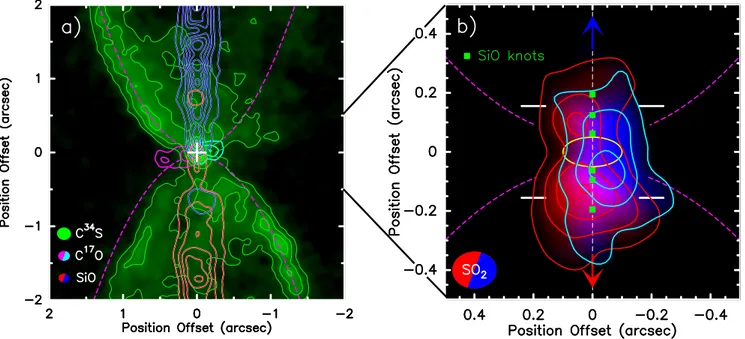
Fig. 1. a: HH212 inner region viewed by ALMA Cycle 4. The SiO jet at | VLS R− Vsys|= 5-10 km s−1(blue and red contours), C17O rotating envelope
at | VLS R− Vsys|= 1.5 km s−1(pink and turquoise), and cavity walls in C34S at | VLS R− Vsys|≤ 0.6km s−1(green, with parabolic fits in dashed magenta)
are shown. First contour and step are 6σ and 18σ for SiO, 6σ and 6σ for C17O, 4σ and 4σ for C34S, where σ is the rms noise level. The source is
shown as a white cross and beam sizes are in the bottom left corner. b: Zoom-in on blue and red SO2at ±2 km s−1shows a slow outflow rotating
in the same sense as the C17O disk. First contour and step are 7σ. White segments show the positions of PV cuts in Fig 2. Green squares show
inner SiO knots imaged by Lee et al. (2017a); the yellow ellipse marks the centrifugal barrier radius at r∼45 au and the height of the COM-rich disk atmosphere at z±20 au (Lee et al. 2017c). Images are rotated such that the vertical axis corresponds to the jet axis at P.A= 22◦
.
of 1km s−1and the lines of SO(98− 87) 346.52848GHz,
SiO(8-7) 347.33063GHz, C34S(7-6) 337.39669GHz, and C17O(3-2)
337.06113GHz with a spectral resolution of 0.1km s−1(rebinned
to 0.44 km s−1). Calibration was carried out following stan-dard procedures under the CASA environment using quasars J0510+1800, J0552+0313, J0541–0211, and J0552–3627. Spec-tral line imaging was performed in CASA with natural weight-ing for C34S to increase sensitivity, resulting in a clean-beam 0.19”×0.17” (PA=-76◦), and with a R=0.5 robust factor for the
other lines, resulting in a beam of 0.15” × 0.13” (PA ∼ -89◦).
The rms noise level is σ ∼ 1 mJy/beam in SO2in 1 km s−1
chan-nels, and σ ∼1.5 mJy/beam in 0.44 km s−1channels for the other
lines. Further data analysis was performed using the GILDAS1 package. Positions are given with respect to the continuum peak at α(J2000)= 05h 43m51s.41, δ(J2000) = –01◦ 0205300. 17 (Lee
et al. 2014) and velocities are with respect to a systemic velocity Vsys= 1.7 km s−1(Lee et al. 2014).
3. Results and discussion
3.1. Evidence for a rotating wide-angle flow in SO and SO2
Figure 1a presents a view of the various components of the HH 212 outflow system from our Cycle 4 data. The chemi-cal stratification first noted by Codella et al. (2014) in Cycle 0 is even more striking: SiO traces the narrow high-velocity jet, while C34S outlines the dense walls of a broad outflow cavity, and C17O traces the rotating equatorial envelope and disk. We
find that the cavity walls may be fitted by a parabolic shape z = r2/a + 0.0500 with a = 0.900 in the north and a = 100 in
the south (slightly less open than sketched in Lee et al. 2017c). Figure 1b presents a zoom on SO2 emission within 0.500=
250 au of the source. This tracer, together with SO, was found
1 http://www.iram.fr/IRAMFR/GILDAS
to be abundant in the HH 212 jet on a larger scale (Podio et al. 2015). Our data resolve its bright emission near the base, reveal-ing a rotation signature in the form of a transverse shift ' ±0.0500
between redshifted and blueshifted emission at ± 2km s−1from systemic, in the same (east-west) sense in both lobes and in the same sense as the envelope rotation in Fig. 1a. The emission peaks at a typical distance of 0.1 − 0.1500, well above the disk
at-mosphere at z ' ±0.0500 traced by complex organic molecules (Lee et al. 2017c; Bianchi et al. 2017) and extends out to ± 0.300along the jet axis, indicating that this rotating material is
outflowing. In the equatorial plane, the emission appears to orig-inate from a region of typical radius ' 0.100= 45 au, i.e., similar
to the centrifugal barrier (herafter CB) estimated from HCO+ infall kinematics, inside which the disk is expected to become Keplerian (Lee et al. 2017c). Channel maps (see Fig. A.1) fur-ther show that this rotating outflow has an onion-like velocity structure with increasing width at progressively lower velocities, which eventually fills up the base of the cavity. The SO emission has a similar behavior (see Fig. A.2). Figure 2 shows transverse position-velocity (PV) cuts and line profiles of SO2 and SO at
±70 au from the midplane (beyond 1 beam diameter, to avoid any contamination by infall). Rotation is clearly apparent as a tilt in the PV cuts. The velocity decrease away from the jet axis is also visible. The centroid velocity in on-axis line profiles, ∼ 1-2km s−1, yields a mean deprojected speed of V
p' 20 − 40km s−1
for an inclination i ' 87◦(Claussen et al. 1998). Hence, the
out-flow cavity is not carved by a fast wide-angle wind at ∼ 100 km s−1, but by a slower component.
3.2. Comparison with MHD disk wind models
We compared the PV cuts and line profiles with synthetic pre-dictions for steady-state, axisymmetric, self-similar DWs from Keplerian disks, calculated following the equations described in Casse & Ferreira (2000). Two key properties of the MHD
so-B. Tabone et al.: ALMA discovery of a rotating SO/ SO2wind in HH212
LETTERS
NATURE ASTRONOMYGaussian profile. For knot S1, the emission at ∼ 4–12 au is unlikely to be from the jet itself and is thus excluded from the fitting. The deconvolved width is the width deconvolved with the beam size of ∼ 8 au (0.02″ ). Knots N2, N3 and S3 have a deconvolved width greater than the beam size. Knots N1, S1 and S2 have a deconvolved width smaller than the beam size.
Mean (or systemic) velocities of the jet. Supplementary Fig. 2 shows the position– velocity diagram of the SiO jet cut along the jet axis. The northern jet component
is detected from ∼ − 14 to 8 km s−1 LSR, with a mean velocity of ∼ − 3 km s−1 LSR
(as indicated by the vertical dashed line). The southern jet component is detected
from ∼ − 5 to 13 km s−1 LSR, with a mean velocity of ∼ 4 km s−1 LSR (as indicated
by the vertical dashed line). These mean velocities are taken to be the systemic velocities in the northern and southern jet components.
Estimation of jet launching radius. Protostellar jets are generally thought to be
launched magneto-centrifugally from disks1. In this framework, the launching
radius of the jet can be derived from the specific angular momentum and the velocity of the jet, based on the conservation of energy and the angular momentum
along the field line, if the mass of the central protostar is known7. For HH 212,
because (1) the jet velocity (poloidal velocity) is so high that the gravitational potential can be neglected at large distances, (2) the jet velocity is much higher
than the jet rotation and (3) the jet inclination angle is very small (∼ 4°)21, the
governing equation (equation (4) in ref. 7) used to derive the jet launching radius
can be simplified and rewritten as:
⎛ ⎝ ⎜⎜ ⎜ ⎞ ⎠ ⎟⎟ ⎟ − − ≈ ⋆ ⋆ l v GMr GM v r 2j 3 0 (1) j 2 0 1/2 j 2 0
to find approximate solutions analytically, where r0 is the launching radius at
the footpoint, υj is the jet velocity, lj is the specific angular momentum of the jet
measured at a large distance, G is the graviational constant and M⋆ is the mass of
the central protostar. Solving this equation, we find the jet launching radius to be:
⎛ ⎝ ⎜⎜ ⎜⎜ ⎜ ⎞ ⎠ ⎟⎟ ⎟⎟ ⎟ ⎡ ⎣ ⎢ ⎢ ⎤ ⎦ ⎥ ⎥ η η ≈ ⋆ − + r l v GM 2 ( ) 1 2 3 1 9 (2) 0 j j 2 2/3 1/3 2
out with two executions in 2015, one on 5 November and the other on 3 December during the Early Science Cycle 3 phase. The projected baselines are 17–16,196 m. The maximum recoverable size scale is ∼ 0.4″ . One pointing was used to map the innermost part of the jet at an angular resolution of 0.02″ (8 au). For the Cycle 1 project, the correlator was set up to have four spectral windows, with one for CO J = 3− 2 at 345.795991 GHz, one for SiO J = 8− 7 at 347.330631 GHz,
one for HCO+ J = 4− 3 at 356.734288 GHz and one for the continuum at 358 GHz
(see Supplementary Table 2). For the Cycle 3 project, the correlator was more flexible and thus was set up to include two more spectral windows, with
one for SO NJ = 89 = 78 at 346.528481 GHz and one for H
13CO+ J = 4− 3 at
346.998338 GHz (see Supplementary Table 3). The total time on the HH 212
system was ∼ 148 minutes.We present here the observational results in SiO, which traces the jet emanating
from the central source. The velocity resolution is 0.212 km s−1 per channel.
However, we binned four channels to have a velocity resolution of 0.848 km s−1 to
map the jet with sufficient sensitivity. The data were calibrated with the Common Astronomy Software Applications (CASA) software package (versions 4.3.1 and 4.5) (https://casa.nrao.edu/) for the passband, flux and gain (see Supplementary Table 4). We used a robust factor of two (natural weighting) for the visibility weighting to generate the SiO maps. To avoid the proper motion effect
(∼ 2 au or 0.005″ per month using 115 km s−1 for the jet velocity22), only Cycle 3 data
were used to study the jet rotation in the innermost part of the jet. This generated a synthesized beam with a size of 0.02″ (8 au) for the maps of the innermost part of the jet (see Fig. 2). To map the knots further out, which are more extended, we also include the Cycle 1 data, which has a larger maximum recoverable scale. In addition, a taper of 0.05″ was used to degrade the beam size to 0.06″ (24 au, see Fig. 1) to improve the signal-to-noise ratio. The noise levels can be measured
from line-free channels and were found to be ∼ 1.6 mJy beam−1 (or ∼ 40 K) for a
beam of ∼ 0.02″ (8 au) and 1.9 mJy beam−1 (or ∼ 6 K) for a beam of ∼ 0.06″ (24 au),
respectively. The velocities in the channel maps and the resulting position–velocity diagrams are LSR.
Gaussian deconvolved width of the jet knots. Supplementary Fig. 1 shows the spatial profile of the jet knots perpendicular to the jet axis, extracted from the SiO total intensity map shown in Fig. 2a (see the white lines for the cuts). To derive the width of the knots, we fitted the spatial profiles of the knots with a
8 a N1 b c d e f East West N2 N3 S1 S2 S3 0 –8 0 –8 8 Position o ff
set for the knot centre (au)
Position velocity cut across the knots in the jet
? ?
0 –8
–15 –10 –5 0 5 10 –5 0 5 10
Observed velocity (km s–1, LSR) Observed velocity (km s–1, LSR)
8 8 0 –8 0 –8 8 0 –8 8
Figure 4 | Position–velocity diagrams cut across the knots (N1–N3 and S1–S3) in the jet. The horizontal dashed lines indicate the peak (central) position of the knots. The vertical dashed lines indicate roughly the systemic (mean) velocities for the northern and southern jet components (as in Fig. 2,
see Methods). The contour levels start from 4σ with a step of 1σ, where σ = 21.3"K. The red contours mark the 7σ detections in knots N2, N3 and S3.
For knots N3 and S1, the emissions marked with a question mark are probably not from the jet itself. The green squares mark the emission peak positions
with > 7σ detections, as determined from the Gaussian fits. The error bars show the uncertainties in the peak positions, which are assumed to be given
by a quarter of the full width at half-maximum. The solid lines mark the linear velocity structures across the knots. The bars indicate the angular
resolution (8"au or ∼ 0.02″) and velocity resolution (∼ 1.7"km"s−1) used for the position–velocity cuts.
Knot N2
MHD-DW: r0= 0.05-0.2 au α = -2 SiO zcut=50aue)
O ffs et fr om kn ot c en te r ( au ) 4© 2017 Macmillan Publishers Limited, part of Springer Nature. All rights reserved. © 2017 Macmillan Publishers Limited, part of Springer Nature. All rights reserved.
NATURE ASTRONOMY 1, 0152 (2017) | DOI: 10.1038/s41550-017-0152 | www.nature.com/nastronomy
LETTERS
NATURE ASTRONOMYGaussian profile. For knot S1, the emission at ∼ 4–12 au is unlikely to be from the jet itself and is thus excluded from the fitting. The deconvolved width is the width deconvolved with the beam size of ∼ 8 au (0.02″ ). Knots N2, N3 and S3 have a deconvolved width greater than the beam size. Knots N1, S1 and S2 have a deconvolved width smaller than the beam size.
Mean (or systemic) velocities of the jet. Supplementary Fig. 2 shows the position– velocity diagram of the SiO jet cut along the jet axis. The northern jet component
is detected from ∼ − 14 to 8 km s−1 LSR, with a mean velocity of ∼ − 3 km s−1 LSR
(as indicated by the vertical dashed line). The southern jet component is detected
from ∼ − 5 to 13 km s−1 LSR, with a mean velocity of ∼ 4 km s−1 LSR (as indicated
by the vertical dashed line). These mean velocities are taken to be the systemic velocities in the northern and southern jet components.
Estimation of jet launching radius. Protostellar jets are generally thought to be
launched magneto-centrifugally from disks1. In this framework, the launching
radius of the jet can be derived from the specific angular momentum and the velocity of the jet, based on the conservation of energy and the angular momentum
along the field line, if the mass of the central protostar is known7. For HH 212,
because (1) the jet velocity (poloidal velocity) is so high that the gravitational potential can be neglected at large distances, (2) the jet velocity is much higher
than the jet rotation and (3) the jet inclination angle is very small (∼ 4°)21, the
governing equation (equation (4) in ref. 7) used to derive the jet launching radius
can be simplified and rewritten as:
⎛ ⎝ ⎜⎜ ⎜ ⎞ ⎠ ⎟⎟ ⎟ − − ≈ ⋆ ⋆ l v GMr GM v r 2j 3 0 (1) j 2 0 1/2 j 2 0
to find approximate solutions analytically, where r0 is the launching radius at
the footpoint, υj is the jet velocity, lj is the specific angular momentum of the jet
measured at a large distance, G is the graviational constant and M⋆ is the mass of
the central protostar. Solving this equation, we find the jet launching radius to be:
⎛ ⎝ ⎜⎜ ⎜⎜ ⎜ ⎞ ⎠ ⎟⎟ ⎟⎟ ⎟ ⎡ ⎣ ⎢ ⎢ ⎤ ⎦ ⎥ ⎥ η η ≈ ⋆ − + r l v GM 2 ( ) 1 2 3 1 9 (2) 0 j j 2 2/3 1/3 2
out with two executions in 2015, one on 5 November and the other on 3 December during the Early Science Cycle 3 phase. The projected baselines are 17–16,196 m. The maximum recoverable size scale is ∼ 0.4″ . One pointing was used to map the innermost part of the jet at an angular resolution of 0.02″ (8 au). For the Cycle 1 project, the correlator was set up to have four spectral windows, with one for CO J = 3− 2 at 345.795991 GHz, one for SiO J = 8− 7 at 347.330631 GHz,
one for HCO+ J = 4− 3 at 356.734288 GHz and one for the continuum at 358 GHz
(see Supplementary Table 2). For the Cycle 3 project, the correlator was more flexible and thus was set up to include two more spectral windows, with
one for SO NJ = 89 = 78 at 346.528481 GHz and one for H
13CO+ J = 4− 3 at
346.998338 GHz (see Supplementary Table 3). The total time on the HH 212
system was ∼ 148 minutes.We present here the observational results in SiO, which traces the jet emanating
from the central source. The velocity resolution is 0.212 km s−1 per channel.
However, we binned four channels to have a velocity resolution of 0.848 km s−1 to
map the jet with sufficient sensitivity. The data were calibrated with the Common Astronomy Software Applications (CASA) software package (versions 4.3.1 and 4.5) (https://casa.nrao.edu/) for the passband, flux and gain (see Supplementary Table 4). We used a robust factor of two (natural weighting) for the visibility weighting to generate the SiO maps. To avoid the proper motion effect
(∼ 2 au or 0.005″ per month using 115 km s−1 for the jet velocity22), only Cycle 3 data
were used to study the jet rotation in the innermost part of the jet. This generated a synthesized beam with a size of 0.02″ (8 au) for the maps of the innermost part of the jet (see Fig. 2). To map the knots further out, which are more extended, we also include the Cycle 1 data, which has a larger maximum recoverable scale. In addition, a taper of 0.05″ was used to degrade the beam size to 0.06″ (24 au, see Fig. 1) to improve the signal-to-noise ratio. The noise levels can be measured
from line-free channels and were found to be ∼ 1.6 mJy beam−1 (or ∼ 40 K) for a
beam of ∼ 0.02″ (8 au) and 1.9 mJy beam−1 (or ∼ 6 K) for a beam of ∼ 0.06″ (24 au),
respectively. The velocities in the channel maps and the resulting position–velocity diagrams are LSR.
Gaussian deconvolved width of the jet knots. Supplementary Fig. 1 shows the spatial profile of the jet knots perpendicular to the jet axis, extracted from the SiO total intensity map shown in Fig. 2a (see the white lines for the cuts). To derive the width of the knots, we fitted the spatial profiles of the knots with a
8 a N1 b c d e f East West N2 N3 S1 S2 S3 0 –8 0 –8 8 Position o ff
set for the knot centre (au)
Position velocity cut across the knots in the jet ? ?
0 –8
–15 –10 –5 0 5 10 –5 0 5 10
Observed velocity (km s–1, LSR) Observed velocity (km s–1, LSR)
8 8 0 –8 0 –8 8 0 –8 8
Figure 4 | Position–velocity diagrams cut across the knots (N1–N3 and S1–S3) in the jet. The horizontal dashed lines indicate the peak (central) position of the knots. The vertical dashed lines indicate roughly the systemic (mean) velocities for the northern and southern jet components (as in Fig. 2,
see Methods). The contour levels start from 4σ with a step of 1σ, where σ = 21.3"K. The red contours mark the 7σ detections in knots N2, N3 and S3.
For knots N3 and S1, the emissions marked with a question mark are probably not from the jet itself. The green squares mark the emission peak positions with > 7σ detections, as determined from the Gaussian fits. The error bars show the uncertainties in the peak positions, which are assumed to be given by a quarter of the full width at half-maximum. The solid lines mark the linear velocity structures across the knots. The bars indicate the angular
resolution (8"au or ∼ 0.02″) and velocity resolution (∼ 1.7"km"s−1) used for the position–velocity cuts.
MHD-DW: r0= 0.1-0.3 au α = -2 SiO zcut=-80au
f)
Knot S3
O ffs et fr om kn ot c en te r ( au )Fig. 2. a-d: Observed on-axis line profiles (histograms) and transverse PV diagrams (color map and white contours) of SO2(left) and SO (middle)
at ±70 au across the northern blue jet (top) and the southern red jet (bottom). The red wing of SO falls outside our spectral set-up. A DW model fit, with λ= 5.5 and W = 30 (see text), is overplotted in black for parameters denoted in each panel. e-f: PV diagrams observed by Lee et al. (2017a) across the SiO knots N2 and S3 (grayscale and black/red contours). Their measured centroids are shown as green squares and fitted rotation gradient as a black line. The DW model is overplotted in cyan (top) or magenta (bottom) with parameters denoted above each panel.
lution affect the predictions. First, the magnetic lever arm pa-rameter λ ' (rA/r0)2, where rA is the Alfvén radius along the
streamline launched from r0, which determines the extracted
an-gular momentum and poloidal acceleration. Second, the maxi-mum widening W = rmax/r0 reached by the streamline, which
controls the flow transverse size. In order to limit the number of free parameters, we kept a fixed inclination i = 87◦ and stellar mass M?= 0.2M (Lee et al. 2017c). The minimum and
maxi-mum launch radii, rinand rout, then determine the range of
veloc-ities in the wind (through the Keplerian scaling). Since initial SO and SO2 abundances at the disk surface are very uncertain, we
did not compute the emissivity from a full thermo-chemical cal-culation along flow streamlines, as carried out for H2O by Yvart
et al. (2016). Instead we assumed a power-law variation with ra-dius ∝ rαwhich allowed us to investigate rapidly a broader range of parameters. Synthetic data cubes were then computed assum-ing optically thin emission and a velocity dispersion of 0.6 km s−1(the sound speed in molecular gas at 100 K), and convolved by a Gaussian beam of the same FWHM as the ALMA clean beam. Parameter α determines the relative weight of inner ver-sus outer streamlines and influences the predicted tilt in the PV. For a given MHD solution, the value of α is well constrained by the slope of the line profile wings.
We find that the DW solution with λ= 13 used to fit the DG Tau jet in Pesenti et al. (2004) is too fast to reproduce the HH212 data; this solution would require an angle from the sky plane of only 0.5◦, outside the observed estimate of 4+3◦
−1◦(Claussen et al.
1998). However, we could obtain a good fit for a slower MHD solution with λ = 5.5 and W = 30. While the emission peaks defining the tilt in PV diagram can be reproduced with rout =
8 au, the more extended emission is better reproduced if we in-crease rout to the expected radius of the Keplerian disk, namely
40 au (Lee et al. 2017c). The corresponding best-fit predictions are superposed in black in Fig 2. The value of rinis constrained
by the highest velocity present in the data; in the blue lobe, the extent of the blue wing suggests rin ≤ 0.1 au. In the red lobe,
our model fit is less good because the centroid is slower than in the blue by a factor 1.5-2. A slower solution with a smaller lever arm (not yet available to us) would probably work better; numerical simulations show that it is indeed possible for a DW to have asymmetric lobes (Fendt & Sheikhnezami 2013). The value rin ' 0.2 au in Figs. 2b,d is thus only illustrative. The
model poloidal speeds at z= 70 au range from ∼ 100 to 2km s−1 for ro= 0.1 to 40 au.
Interestingly, we find that the same DW solution that fits the SO and SO2 PV cuts can also reproduce the rotation
sig-natures across axial SiO knots at similar altitude, if SiO traces only inner streamlines launched from 0.05-0.1 au to 0.2-0.3 au. This is shown in Fig. 2e-f, where our synthetic predictions, con-volved by 8 au are compared with the ALMA SiO data of Lee et al. (2017a). The predicted range of terminal speeds is 70-170km s−1, which is consistent with SiO proper motions. Since
the dust sublimation radius is also 0.2-0.3 au (Yvart et al. 2016), SiO would be released by dust evaporation at the wind base.
A&A proofs: manuscript no. main
3.3. Biases in analytical estimates of DW outer launch radius An unexpected result is that our best fitting rout ' 0.2 − 0.3 au
for SiO knots is 2-10 times larger than the 0.05+0.05−0.02au estimated by Lee et al. (2017a) with the Anderson et al. (2003) formula, which is valid for all steady DWs. Since the knots are resolved, this cannot be due to beam smearing as in the cases investigated by Pesenti et al. (2014). The same applies to our SO and SO2
PV cuts, whereas inserting the apparent velocity gradient in the Anderson formula would give rout ∼ 1 au instead of 40 au. We
explored the reason for this discrepancy and found that the su-perposition of many flow surfaces along the line of sight creates a shallower velocity gradient leading to strongly underestimate rout. A detailed study of this effect, which also leads to
underes-timating λ, will be presented in Tabone et al. (in prep).
3.4. Further model tests and limitations
A strong test of the DW picture would be to detect the predicted helical magnetic field structure, for example, through dust polar-ization measurements with ALMA. Figure 3 plots the poloidal magnetic surfaces in our best-fit model. Beyond the Alfvén sur-face (at z/r0 ' 2), a strong toroidal field develops. In the disk
atmosphere at z ∼ 20 au, brightest in dust continuum, the ratio of toroidal to poloidal magnetic field Bφ/Bpranges from 1.5 to
10, from outer to inner streamlines. Hence, polarization maps (if not dominated by dust scattering) should not show a pure "hour-glass" geometry but be more toroidal closer to the axis.
We also caution that our DW modeling is only illustrative, owing to its simplifications. Notably, self-similarity cannot prop-erly treat the effect of outer truncation. In reality, the shape and dynamics of the last DW streamlines would be determined by pressure balance with the cavity and infalling envelope. As de-picted in Figure 3, they would thus open in the cavity more widely than predicted. This wider opening might explain the broader SO and SO2 emission beyond the last model contour
in PV diagrams and the slow HCO+ wind noted by Lee et al. (2017c). The opposite pressure effect occurs near the equator, where the thick infalling stream would confine the streamlines inside the CB more tightly than in our model. As shown in Fig. 3, the heating resulting from this interaction might naturally ex-plain the presence of a warm ring of COM emission close to the centrifugal barrier (Lee et al. 2017c; Bianchi et al. 2017). DW models including these effects remain to be developed.
4. Conclusions
Our Cycle 4 ALMA data reveal a rotating wide-angle flow in SO and SO2 around the SiO jet with a mean speed of ∼ 30 km s−1
and an onion-like velocity structure filling in the base of the out-flow cavity. Hence, the cavity is not carved by a fast wide-angle wind, but by a slower component. This component emerges from within and up to the centrifugal barrier, and contributes to re-move excess angular momentum and mass from this region.
The observed kinematics set tight constraints on stationary, self-similar MHD disk wind models. The lever arm parameter λ should be <∼ 5, smaller than in the atomic DG Tau rotating flow (Pesenti et al. 2004), and the launch radii would range from 0.05 to ∼ 40 au, with SiO tracing only dust-free streamlines launched up to 0.2-0.3 au. If such a disk wind is extracting most of the an-gular momentum required for disk accretion, it would be
eject-HCO + wind ? Infall
CB
Dust diskSO, SO
2SiO
COMsFig. 3. Schematic view of the inner 180 au of the HH212 system follow-ing our MHD disk-wind modelfollow-ing. The streamlines rich in SiO are pic-tured in green, the wider component traced by SO and SO2is in black,
for launch radii of 0.25, 0.9, 3, 11, and 40 au. The magenta dashed curve shows the boundary of the cavity from Fig. 1. The dusty disk scale height from Lee et al. (2017b) is indicated in blue, the centrifugal barrier in red, and the COMs warm ring in orange (Lee et al. 2017c; Bianchi et al. 2017).
ing 50% of the incoming accretion flow2. If this is widespread among low-mass protostars, as suggested by H2O line profiles
(Yvart et al. 2016), this component could strongly contribute to the low core-to-star efficiency ' 30% (eg. André et al. 2010). We nevertheless caution that our modeling is very idealized and probably not unique. Higher angular resolution and dust polar-ization maps with ALMA could provide powerful tests of this scenario.
Finally, an important side result of our study is that the ap-parent rotation gradient strongly underestimates the actual out-ermost launch radius of an extended MHD disk wind. A de-tailed study of the magnitude of this effect, which applies beyond HH 212, will be presented in Tabone et al. (in prep).
Acknowledgements. We are very grateful to K.L.J. Rygl for her support with data reduction at the Bologna ARC node, and we thank the anonymous ref-eree for useful comments. This paper makes use of the ALMA 2016.1.01475.S data (PI: C. Codella). ALMA is a partnership of ESO (representing its mem-ber states), NSF (USA), and NINS (Japan), together with NRC (Canada) and NSC and ASIAA (Taiwan), in cooperation with the Republic of Chile. The Joint ALMA Observatory is operated by ESO, AUI/NRAO, and NAOJ. This work was supported by the Programme National “Physique et Chimie du Milieu Interstel-laire” (PCMI) of CNRS/INSU with INC/INP and co-funded by CNES, and by the Conseil Scientifique of Observatoire de Paris. This research has made use of NASA’s Astrophysics Data System.
References
Anderson, J. M., Li, Z.-Y., Krasnopolsky, R., & Blandford, R. D. 2003, ApJ, 590, L107
André, P., Men’shchikov, A., Bontemps, S., et al. 2010, A&A, 518, L102 Bacciotti, F., Ray, T. P., Mundt, R., Eislöffel, J., & Solf, J. 2002, ApJ, 576, 222 Béthune, W., Lesur, G., & Ferreira, J. 2017, A&A, 600, A75
Bianchi, E., Codella, C., Ceccarelli, C., et al. 2017, ArXiv e-prints
Bjerkeli, P., van der Wiel, M. H. D., Harsono, D., Ramsey, J. P., & Jørgensen, J. K. 2016, Nature, 540, 406
Casse, F. & Ferreira, J. 2000, A&A, 353, 1115
Claussen, M. J., Marvel, K. B., Wootten, A., & Wilking, B. A. 1998, ApJ, 507, L79
Codella, C., Cabrit, S., Gueth, F., et al. 2014, A&A, 568, L5
2 M˙
ej/ ˙Macc(rout)=
h
1 − (rin/rout)ξ
i
with ξ ' 1/(2λ − 2) when the wind braking torque dominates (Casse & Ferreira 2000)
Fendt, C. & Sheikhnezami, S. 2013, ApJ, 774, 12
Ferreira, J., Dougados, C., & Cabrit, S. 2006, A&A, 453, 785
Hirota, T., Machida, M. N., Matsushita, Y., et al. 2017, Nature Astronomy, 1, 0146
Launhardt, R., Pavlyuchenkov, Y., Gueth, F., et al. 2009, A&A, 494, 147 Lee, C.-F., Hirano, N., Zhang, Q., et al. 2014, ApJ, 786, 114
Lee, C.-F., Ho, P. T. P., Li, Z.-Y., et al. 2017a, Nature Astronomy, 1, 0152 Lee, C.-F., Li, Z.-Y., Ho, P. T. P., et al. 2017b, Science Advances, 3, e1602935 Lee, C.-F., Li, Z.-Y., Ho, P. T. P., et al. 2017c, ApJ, 843, 27
Louvet, F., Dougados, C., Cabrit, S., et al. 2016, A&A, 596, A88 Matthews, L. D., Greenhill, L. J., Goddi, C., et al. 2010, ApJ, 708, 80 Panoglou, D., Cabrit, S., Pineau Des Forêts, G., et al. 2012, A&A, 538, A2 Pesenti, N., Dougados, C., Cabrit, S., et al. 2004, A&A, 416, L9
Podio, L., Codella, C., Gueth, F., et al. 2015, A&A, 581, A85
Yvart, W., Cabrit, S., Pineau des Forêts, G., & Ferreira, J. 2016, A&A, 585, A74 Zhu, Z. & Stone, J. M. 2017, ArXiv:1701.04627
A&A proofs: manuscript no. main
Fig. A.1. Channel maps of continuum-subtracted SO28(2, 6) − 7(1, 7) emission within ±0.500of the central source of HH212. The velocity offset
from the systemic velocity (Vsys = 1.7km s−1) is indicated (in km s−1) in the upper right corner with blue and red contours denoting blueshifted
and redshifted emission. The channel width is 1 km s−1. First contour and steps corresponds to 4σ and 6σ (σ=1mJy/beam), respectively. The C34S
Fig. A.2. Channel maps of continuum-subtracted SO 98− 87emission within ±0.500 of the central source of HH212. The velocity offset from
the systemic velocity (Vsys = 1.7km s−1) is indicated (in km s−1) in the upper right corner with blue and red contours denoting blueshifted and
redshifted emission. The channel width is 0.44 km s−1. First contour and steps corresponds to 6σ and 16σ (σ=1.7mJy/beam), respectively. The