Alma Mater Studiorum – Università di Bologna
DOTTORATO DI RICERCA IN
Disegno e Metodi dell’Ingegneria Industriale
e Scienze Aerospaziali
Ciclo XXVI
Settore Concorsuale di afferenza: 09/A1 Ingegneria Aeronautica, Aerospaziale e Navale Settore Scientifico disciplinare: ING-IND/05 Impianti e Sistemi Aerospaziali
TITOLO TESI
DEVELOPMENT OF NEW TOOLKITS
FOR ORBIT DETERMINATION CODES
FOR PRECISE RADIO TRACKING EXPERIMENTS
Presentata da: Marco Zannoni
Coordinatore Dottorato
Relatore
Prof. Vincenzo Parenti Castelli
Prof. Paolo Tortora
Author’s Note
This thesis is continuously revised to correct all the errors that are found during a never-ending revision process. To obtain the most updated version, please feel free to contact the author by sending an e-mail at: [email protected].
Summary
This thesis describes the developments of new models and toolkits for the orbit determination codes to support and improve the precise radio tracking experiments of the Cassini-Huygens mission.
Cassini-Huygens is a joint NASA/ESA/ASI interplanetary mission dedicated to the study of the Saturn’s planetary system which, composed by the planet Saturn itself, its natural satellites and rings, is one of the most complex and interesting planetary systems known. In the mission context, the radio science subsystem provides fundamental information about the Saturn’s rings, its atmosphere and ionosphere and the gravity fields of Saturn and its main satellites. In particular, the determination of the gravity field of a celestial body plays a crucial role in the investigation of its internal composition, structure and evolution, because it provides one of the very few direct measurements of its internal mass distribution, even if with various limitations. The gravity radio science is a particular application of the precise orbit determination of an interplanetary spacecraft, which consists in the estimation of a set of parameters that unambiguously defines its trajectory. The core of the process is the comparison between measured observables and the corresponding computed values, obtained by an orbit determination program using the adopted mathematical models. Hence, disturbances in either the observed or computed observables degrades the orbit determination process. While the different sources of noise in the Doppler measurements were the subject of several studies in the past, the errors in the computed Doppler observables were not previously analyzed and characterized in details.
Chapter 2 describes a detailed study of the numerical errors in the Doppler observables computed by the most important interplanetary orbit determination pro-grams: NASA/JPL’s ODP (Orbit Determination Program) and MONTE (Mission-analysis, Operations, and Navigation Toolkit Environment), and ESA/ESOC’s AMFIN (Advanced Modular Facility for Interplanetary Navigation). During this study a mathematical model of the numerical noise was developed. The model was successfully validated analyzing directly the numerical noise in Doppler observables computed by the ODP and MONTE, showing a relative error always smaller than 50%, with typical values better than 10%. An accurate prediction of the numer-ical noise can be used to compute a proper noise budget in Doppler tracking of interplanetary spacecraft. This represents a critical step for the design of future interplanetary missions, both for radio science experiments, requiring the highest level of accuracy, and spacecraft navigation. As a result, the numerical noise proved to be, in general, an important source of noise in the orbit determination process and, in some conditions, it may becomes the dominant noise source. On the basis
of the numerical errors characterization, three different approaches to reduce the numerical noise were proposed.
MONTE is the new orbit determination software developed since late 2000s by the NASA/JPL. Only recently it was considered sufficiently stable to completely replace the ODP for the orbit determination of all the operational missions managed by the JPL. In parallel, MONTE replaced the ODP also for the analysis of radio science gravity experiment, so new set-ups, toolkits and procedures were developed to perform this task. In particular, to analyze the data acquired during the Cassini gravity radio science experiments the use of a multi-arc procedure is crucial while, at present, MONTE supports only a single-arc approach. Chapter 3 describes the development of the multiarc MONTE-Python library, which allows to extend the Monte capabilities to perform a multi-arc orbit determination. The library was developed and successfully tested during the analysis of the Cassini radio science gravity experiments of the Saturn’s satellite Rhea.
Discovered on 1672 by Giovanni Domenico Cassini, Rhea is the second largest moon of Saturn. Before the Cassini arrival to Saturn, only the gravitational parameter GM was known, from the analysis of Pioneer and Voyager data. During its mission in the Saturn’s system, Cassini encountered Rhea four times, but only two flybys were devoted to gravity investigations. The first gravity flyby, referred to as R1 according to the numbering scheme used by the project Cassini, was performed on November 2005. The radiometric data acquired during this encounter were analyzed by the scientific community with two different approaches, obtaining non-compatible estimations of the Rhea’s gravity field. A first approach assumed a
priori the hydrostatic equilibrium, deriving that Rhea’s interior is a homogeneous,
undifferentiated mixture of ice and rock, with possibly some compression of the ice and transition from ice I and ice II at depth. A second approach computed an unconstrained estimation of the quadrupole gravity field coefficients J2, C22 and S22,
obtaining a solution non statistically compatible with the condition of hydrostatic equilibrium. In this case, no useful constraint on Rhea’s interior structure could be imposed. To resolve these discrepancies, a second and last gravity fly-by of Rhea, referred to as R4, was performed on March 2013. Chapter 4 presents the estimation of the Rhea’s gravity field obtained from a joint multi-arc analysis of R1 and R4, describing in details the spacecraft dynamical model used, the data selection and calibration procedure, and the analysis method followed. In particular, the approach of estimating the full unconstrained quadrupole gravity field was followed, obtaining a solution statistically not compatible with the condition of hydrostatic equilibrium. To test the stability of the solution, different multi-arc analysis were performed, varying the data set, the strategy for the update of the satellite ephemerides and the dynamical model. The solution proved to be stable and reliable. Given the non-hydrostaticity, very few considerations about the internal structure of Rhea can be made. In particular, the computation of the moment of inertia factor using the Radau-Darwin equation can introduce large errors. Nonetheless, even by accounting for this possible error, the normalized moment of inertia is in the range 0.37-0.4 indicating that Rhea’s may be almost homogeneous, or at least characterized by a small degree of differentiation. The internal composition cannot be assessed with more details with the available data but, unfortunately, no other gravity flybys are scheduled up to the end of the mission in 2017.
Sommario
Questa tesi descrive lo sviluppo di nuovi modelli e strumenti per codici di determinazion orbitale, per supportare e migliorare gli esperimenti di radio tracking della missione Cassini-Huygens.
Cassini-Huygens è una missione spaziale interplanetaria dedicata allo studio del sistema planetario di Saturno che, costituito dallo stesso pianeta Saturn, dalle sue lune e dagli anelli, è uno dei sistemi planetari più complessi ed interessanti del sistema solare. In questo contesto, il sottosistema di Radio Scienza fornisce misure fondamentali degli anelli di Saturno, la sua atmosfera e ionosfera, e dei campi gravitazionali di Saturno e dei suoi satelliti principali. In particolare, la determinazione del campo di gravità di un corpo celeste ha un ruolo cruciale nello studio della sua composizione interna, struttura ed evoluzione, in quanto costituisce uno delle pochissime misure dirette della distribuzione interna della sua massa, anche se non attraverso una relazione univoca. Gli esperimenti di radio scienza dedicati alla gravità rappresentano una particolare applicazione del processo di determinazione orbitale di un veicolo spaziale interplanetario, che consiste nella stima di un insieme di parametri che definisce univocamente la sua traiettoria. Il processo di stima è basato sulla comparazione tra le reali misure ottenute a terra e i corrispondenti valori simulati usando dei modelli matematici. Di conseguenza, la stima viene degradata sia da errori sulle misure, sia da errori sulle osservabili simulate. Mentre le diverse sorgenti di rumore di misura sono state oggetto in passato di diversi studi, gli errori sulle osservabili simulate non sono stati mai analizzati in dettaglio.
Il Capitolo 2 descrive uno studio approfondito dei rumori numerici che carat-terizzano le osservabili calcolate attraverso i principali software di determinazione orbitale: ODP e MONTE del NASA/JPL, e AMFIN di ESA/ESOC. Durante questo studio un modello matematico del rumore numerico è stato sviluppato. Il modello è stato validato analizzato direttamente il rumore numerico sulle osservabili Doppler calcolate da ODP e da MONTE, mostrando un errore relativo sempre inferiore al 50%, con valori tipici inferiori al 10%. Una predizione accurata del rumore numerico può essere usata per calcolare un più accurato noise budget del tracking Doppler di missioni interplanetarie. Questo rappresenta un aspetto critico nello sviluppo di future missioni, sia per la navigazione, sia per gli esperimenti di radio scienza, che richiedono le accuratezze più elevate. In generale, il rumore numerico si è rivelato essere un’importante sorgente di rumore nel processo di determinazione orbitale e, in alcune condizioni, può rappresentare la sorgente di rumore dominante. La caratterizzazione del rumore numerico ha permesso di identificare tre possibili approcci per ridurre il rumore numerico.
MONTE è il nuovo software di determinazione orbitale sviluppato sin dalla fine degli anni 2000 dal NASA/JPL. Solo recentemente MONTE è stato considerato sufficientemente stabile per sostituire completamente ODP nella determinazione orbitale delle missioni operative gestite dal JPL. Di conseguenza, MONTE ha sostituito ODP anche nell’analisi degli esperimenti di radio scienza, e a questo scopo nuovi set-up, strumenti e procedure sono stati sviluppati. In particolare, l’utilizzo del metodo multi-arco è fondamentale per l’analisi dei dati acquisiti durante gli esperimenti di radio scienza di Cassini dedicati alla gravità ma, attualmente, MONTE supporta solo il metodo singolo arco. Il Capitolo 3 descrive lo sviluppo e le caratteristiche della libreria MONTE-Python multiarc, che permette di estendere le funzionalità di Monte per effettuare analisi multi-arco. La libreria è stata sviluppata e testata durante l’analisi degli esperimenti di radio scienza di Cassini dedicati alla stima del campo di gravità di Rea.
Scoperto nel 1672 da Giovanni Domenico Cassini, Rea è il secondo più grande satellite di Saturno. Prima dell’arrivo della missione Cassini a Saturno, solo il
GM di Rea era noto, attraverso l’analisi dei dati delle missioni Pioneer e Voyager.
Durante la missione di Cassini nel sistema di Saturno, sono stati realizzati quattro
fly-bys di Rea, di cui solo due dedicati alla stima del campo di gravità. Il primo
fly-by, denominato R1 secondo lo schema di numerazione usato dal progetto Cassini, è stato effettuato nel Novembre 2005. I dati raccolti durante questo incontro sono stati analizzati dalla comunità scientifica utilizzando due approcci differenti, ottenendo stime del campo di gravità differenti e non compatibili tra loro. Una prima soluzione fu ottenuta assumendo a priori la condizione di equilibrio idrostatico, deducendo che Rhea è un miscuglio omogeneo, non differenziato, di ghiaccio e roccia, con una possibile presenza di compressione del ghiaccio e transizione in profondità da ghiaccio I a ghiaccio II. Una seconda soluzione, ottenuta stimando un i coefficienti del campo di quadrupolo J2, C22 e S22 senza alcun vincolo, risultò
non essere statisticamente compatibile con la condizione di equilibrio idrostatico. Di conseguenza alcun vincolo sulla possibile struttura interna di Rea potè essere imposto. Per risolvere questo disaccordo, un secondo e ultimo fly-by di Rea, denominato R4, fu pianificato ed eseguito nel Marzo 2013. Il Capitolo 4 presenta la stima dela campo di gravità di Rea ottenuta dall’analisi dati congiunta di R1 e R4, descrivendo in dettaglio il modello dinamico della sonda utilizzato, la procedure di selezione e calibrazione dei dati, e il metodo di analisi adottato. In particolare, si è scelto di stimare l’intero campo gravitazionale di quadrupolo, senza alcun vincolo
a priori, ottenendo una soluzione non compatibile con la condizione di equilibrio
idrostatico. Per testare la stabilità della soluzione diverse analisi multi-arco sono state realizzate, modificando i dati analizzati, la strategia di aggiornamento delle effemeridi satellitari e il modello dinamico. La soluzione si è dimostrata stabile e affidabile. Data la condizione non idrostatica, poche considerazioni possono essere fatte sull struttura interna di Rea. In particolare, il calcolo del momento di inerzia utilizzando l’equazione di Radau-Darwin non è del tutto affidabile. Nonstante ciò, anche considerando i possibili errori, il momento di inerzia normalizzato ottenuto si trova nel range 0.37-0.4, indicando che Rea potrebbe essere omogoneo, o almeno con un basso livello di differenziazione. Tuttavia, la composizione interna non può essere valutata più in dettaglio con i dati disponibili e, sfortunatamente, non sono previsti altri fly-by di Rea dedicati alla gravità fino alla fine della missione nel 2017.
Contents
Acronyms xix
1 Introduction 1
1.1 The Cassini-Huygens Mission . . . 1
1.1.1 The Scientific Objectives . . . 2
1.1.2 The Cassini Mission . . . 3
1.1.3 The Cassini-Huygens Spacecraft . . . 4
1.1.4 The Cassini Radio Science Subsystem . . . 6
1.1.4.1 Scientific Objectives . . . 6
1.1.4.2 Overview . . . 7
1.1.4.3 Spacecraft Segment . . . 8
1.1.4.4 Ground Segment . . . 10
1.2 The Orbit Determination Problem . . . 12
1.2.1 Introduction . . . 12
1.2.2 Pre-processing of radiometric measurements . . . 13
1.2.3 Observables and partials computation . . . 14
1.2.3.1 Planetary and/or Satellite ephemerides update . . 14
1.2.3.2 Trajectory Integration . . . 15
1.2.3.3 Time transformations . . . 16
1.2.3.4 Ground station state computation . . . 17
1.2.3.5 Light-time solution computation . . . 18
1.2.3.6 Observables computation . . . 18
1.2.4 Estimation Filter . . . 19
1.2.5 Solution Analysis . . . 19
2 Numerical Noise 21 2.1 Introduction . . . 21
2.2 The Round-Off Errors . . . 23
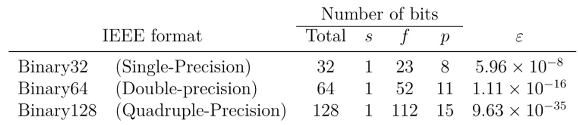
2.2.1 The Floating Point Representation . . . 23
2.2.1.1 The Effect of the Measurement Units . . . 25
2.2.2 The Statistical Model . . . 26
2.2.3 Operation Errors . . . 27
2.3 The Numerical Error Model . . . 28
2.3.1 Differenced-Range Doppler Formulation . . . 28
2.3.2 Sources of Numerical Errors and Order of Magnitude Consid-erations . . . 30
2.3.2.1 Representation of Times . . . 30
2.3.2.2 Representation of Distances . . . 32
2.3.2.3 Additional Rounding Errors . . . 32
2.3.3 Numerical Error Preliminary Model . . . 33
2.3.4 Validation of the Widrow’s Model . . . 35
2.3.5 Numerical Error Complete Model . . . 37
2.4 Model Validation . . . 38
2.4.1 Validation Procedure . . . 38
2.4.2 The Six-Parameter Fit . . . 39
2.4.3 Validation Results . . . 40
2.4.3.1 ODP . . . 40
2.4.3.2 MONTE . . . 44
2.4.4 Validation Conclusions . . . 49
2.5 Numerical Noise Analysis . . . 49
2.5.1 ODP Numerical Noise . . . 50
2.5.2 MONTE Numerical Noise . . . 54
2.6 Numerical Noise Mitigation . . . 54
2.7 Conclusions . . . 58
3 Multi-Arc Toolkit 59 3.1 Introduction . . . 59
3.2 The Single-Arc Approach . . . 59
3.3 The Multi-Arc Approach . . . 61
3.4 The Multi-Arc Monte Library . . . 62
3.4.1 Implementation . . . 62
3.4.1.1 The “external” approach . . . 62
3.4.1.2 The “multi-spacecraft” approach . . . 62
3.4.1.3 The “hybrid” approach . . . 63
3.4.2 The Multi-Arc Analysis Procedure . . . 64
3.4.3 Set-Up of a Multi-Arc Analysis . . . 66
3.4.3.1 Create the Multi-Arc Directory . . . 66
3.4.3.2 Add and Configure the Single Arcs . . . 67
3.4.3.3 Configure the Multi-Arc Options.mpy . . . 68
3.4.3.4 Configure the Multi-Arc Setup File . . . 68
3.4.3.5 Configure the Multi-Arc Filter . . . 69
3.4.4 Analysis Execution . . . 70
3.4.5 Current Limitations . . . 70
3.5 Conclusions and Future Work . . . 70
4 Rhea Gravity Field 73 4.1 Introduction . . . 73
4.2 Dynamical Model . . . 76
4.2.1 Gravitational Accelerations . . . 77
4.2.1.1 Rhea Rotation Model . . . 77
4.2.2 Non-Gravitational Accelerations . . . 78
4.2.2.1 Meneuvers . . . 79
4.2.2.2 RTGs . . . 79
CONTENTS xiii
4.2.2.4 Saturn Albedo . . . 80
4.2.2.5 Atmospheric Drag . . . 80
4.3 Satellite Ephemerides Update . . . 80
4.4 Data . . . 82
4.4.1 Data Selection . . . 82
4.4.2 Data Calibration . . . 83
4.4.2.1 Time synchronization of AMC data . . . 83
4.5 Estimation . . . 86
4.6 Results . . . 88
4.6.1 Residuals . . . 88
4.6.2 Rhea Gravity Field . . . 89
4.6.3 Comments . . . 89
4.6.3.1 MONTE Set-Up Validation . . . 89
4.6.3.2 The Multi-Arc Strategy . . . 97
4.6.3.3 The Satellite Ephemerides Update Strategy . . . . 98
4.7 Interpretation . . . 98
5 Conclusions 101
List of Figures
1.1 The Cassini-Huygens spacecraft in cruise configuration. . . 5
2.1 Round-off errors in time variables for ODP, AMFIN and MONTE. . 31
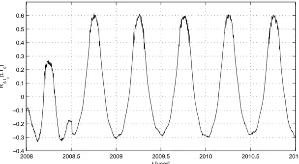
2.2 Autocorrelation of ∆t3, computed on different tracking passes. . . . 37
2.3 Time variation of the autocorrelation of ∆t3 after Tc= 60 s. . . 38
2.4 ODP numerical noise residuals. . . 41
2.5 ODP numerical noise standard deviation: Cassini scenario. . . 42
2.6 ODP numerical noise standard deviation: Juno scenario. . . 43
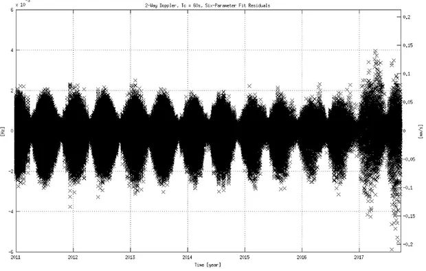
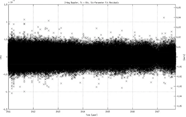
2.7 MONTE numerical noise residuals. . . 45
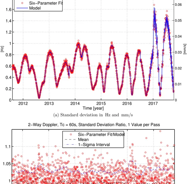
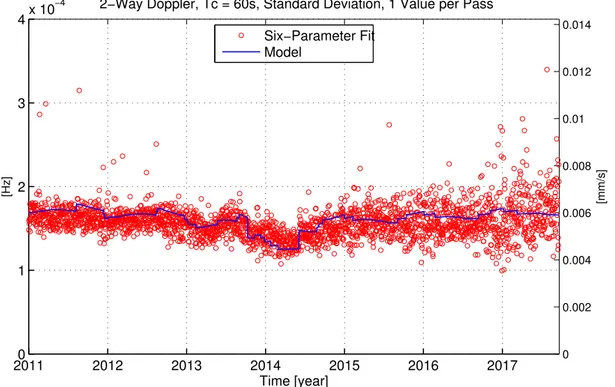
2.8 MONTE numerical noise residuals: Juno scenario (bad points zoom). 46 2.9 MONTE numerical noise standard deviation: Cassini Scenario. . . . 47
2.10 MONTE numerical noise standard deviation: Juno Scenario. . . 48
2.11 ODP numerical noise: Cassini cruise phase. . . 51
2.12 ODP numerical noise: Cassini Nominal and Equinox Missions. . . . 51
2.13 ODP numerical noise: Cassini Solstice Mission. . . 52
2.14 ODP numerical noise: Juno Nominal Mission. . . 52
2.15 MONTE numerical noise: Cassini cruise phase. . . 55
2.16 MONTE numerical noise: Cassini Nominal and Equinox Missions. . 55
2.17 MONTE numerical noise: Cassini Solstice Mission. . . 56
2.18 MONTE numerical noise: Juno Nominal Mission. . . 56
3.1 multiarc library: block diagram of the multi-arc procedure. . . 65
4.1 Estimations of Rhea J2 and C22 published to date. . . 75
4.2 Rhea R1 and R4 ground tracks. . . 76
4.3 Cassini elevation during R1 and R4. . . 84
4.4 R4 AMC on DSS-55: cross-correlation with residuals. . . 85
4.5 R4 AMC on DSS-25: cross-correlation with residuals. . . 86
4.6 Sol-R1 and Sol-R4: range-rate residuals. . . 90
4.7 Sol-MA-0: range-rate residuals. . . 91
4.8 Sol-MA: range-rate residuals. . . 92
4.9 Sol-MA-L: range-rate residuals. . . 93
4.10 Sol-MA-HE: range-rate residuals. . . 94
4.11 Rhea GM 1-sigma error bars. . . . 95
4.12 Rhea J2-C22 1-sigma error ellipses. . . 95
4.13 Rhea J2/C22− 10/3 1-sigma error bars. . . . 97
List of Tables
2.1 Binary formats defined by IEEE-754. . . 25
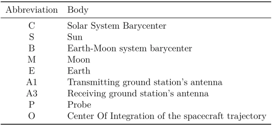
2.2 List of bodies abbreviations. . . 29
4.1 Rhea characteristics. . . 73
4.2 R1 and R4 characteristics. . . 75
4.3 Coefficients defining the Cassini RTG acceleration. . . 80
4.4 Rhea estimated gravity fields. . . 96
4.5 Rhea Fluid Love’s Number and C/M R2. . . 100
Acronyms
AMC Advanced Media Calibration system
ASD Allan Standard Deviation
AV Allan Variance
AWVR Advanced Water Vapour Radiometer
BWG Beam Wave Guided Antenna
C/A Closest Approach
CSO Cryogenically-cooled Sapphire Oscillator
DDOR Delta Differential One-way Ranging
DOR Differential One-way Ranging
DRVID Differenced Range Versus Integrated Doppler
DSN Deep Space Network
DSS Deep Space Station
ECEF Earth-Centered Earth-Fixed
ECI Earth-Centered Inertial
ERT Earth Received Time
ESA European Space Agency
ESTRACK ESA Tracking Stations Network ET Ephemeris Time
GMT Greenwich Mean Time
GPS Global Positioning System
GRV GRaVity
GSE Gravity Science Enhancement
HEA High Efficiency Antenna
IAU International Astronomical Union
ICRF International Celestial Reference Frame
IERS International Earth Rotation Service
ITRF International Terrestrial Reference Frame
JPL Jet Propulsion Laboratory
LITS Linear Ion Trap Standard
LOS Line Of Sight
MONTE Mission-analysis, Operations, and Navigation Toolkit Environment
MWR Micro-Wave Radiometer
ODP Orbit Determination Program
OWLT One-Way Light Time
PLL Phase-Locked Loop
PN Pseudo-random Noise
RMS Root Mean Square
RTTT Round-Trip Transit Time
RTLT Round-Trip Light Time
RU Range Units
SCET SpaceCraft Event Time
SEP Sun-Earth-Probe angle
SNR Signal to Noise Ratio
SOS Sum Of Square
SRA Sequential Ranging Assembly
SRP Solar Radiation Pressure
ST Station Time
SVD Singular Value Decomposition
TAI International Atomic Time
TDB Barycentric Dynamical Time
xxi
TSAC Tracking System Analitical Calibration
TWLT Two-Way Light Time
USO Ultra-Stable Oscillator
UTC Coordinated Universal Time
UT Universal Time
VLBI Very Long Baseline Interferometry
Chapter 1
Introduction
1.1
The Cassini-Huygens Mission
Cassini-Huygens is a joint NASA/ESA/ASI interplanetary mission with the primary goal to conduct an in-depth exploration of the Saturn’s system. NASA supplied the Cassini orbiter, ESA supplied the Huygens Titan probe, and ASI provided hardware systems for the orbiter as well as instruments for both the orbiter and probe. The primary goal of Cassini is to conduct an in-depth exploration of the Saturn system. The orbiter was named after the Italian astronomer Giovanni Domenico Cassini (1625-1712), who discovered the Saturn’s satellites Iapetus, Rhea, Dione and Tethys, and who firstly noted rings features such as the Cassini division. The probe was named after the dutch astronomer Christiaan Huygens (1629-1695), who discovered the first moon of Saturn, Titan, using a self-made telescope.
Being visible to the naked eye, Saturn is known since the ancient times. Saturn is the second most massive planet in the Solar System, and its system is one of the most complex and extraordinary planetary systems known. It is composed by:
• The planet Saturn itself, with its atmosphere, gravity field, magnetic field. • Titan, the biggest moon of Saturn, the second in the solar system.
• The icy satellites, among which Enceladus, Dione and Rhea are the most important.
• The rings system, the largest and most developed in the solar system. • The Saturn magnetosphere.
Cassini is studying the present status of each element, the processes operating on or in them, and the interactions between them, on short and large time scales, allowing to characterize also the seasonal variations during almost half of the 30-year Saturn revolution period.
Our understanding of the Saturn system has been greatly enhanced by the Cassini-Huygens mission. Fundamental discoveries have altered our views of Saturn, Titan and the icy moons, the rings, and magnetosphere of the system.
1.1.1
The Scientific Objectives
In this section an overview of the scientific objectives of the Cassini-Huygens mission is provided, for each element of the Saturn system [44].
Titan Titan is the major focus of the mission. It is studied by both the Cassini orbiter and the Huygens probe. Second for dimensions, Titan has the thickest atmosphere among the satellites in the Solar System. Moreover, Titan is the only object in the solar system other than Earth that sustains an active hydrological cycle with surface liquids, most liquid methane and ethane, meteorology, and climate change. It possesses methane-ethane lakes and seas, fluvial erosion, and equatorial dunes shaped by winds and formed of organic particles derived from methane. The main scientific objectives related to Titan of the mission are:
• Determine the composition of the atmosphere, constraining scenarios of the formation and evolution of Titan and its atmosphere.
• Characterize the atmosphere, chemically, energetically, measuring winds and global temperatures, and observing the seasonal effects.
• Determine the topography and surface composition. • Infer the internal structure of the satellite.
• Investigate the upper atmosphere, and its role as a source of neutral and ions materials for the magnetosphere of Saturn.
Icy Satellites Saturn has a large number of satellites, with sizes varying from several km to hundreds of km. As satellites become smaller they approach the size of ring particles. Some of the smaller icy satellites are embedded into the rings and interact with them creating complex and fascinating patterns. Among the icy satellites, the Cassini’s discovery of ongoing endogenic activity of Enceladus was extremely important- The Cassini scientific objectives specific to the icy satellites are:
• Determine the general characteristics and geological histories of the satellites. • Define the mechanisms, both external and internal, responsible of crustal and
surface modifications.
• Investigate the composition and distribution of surface materials.
• Constrain models of the satellites bulk composition and internal structures. • Investigate interactions with the magnetosphere and ring system, as possible
1.1. THE CASSINI-HUYGENS MISSION 3
Magnetosphere The scientific objectives specific to magnetospheric and plasma science are:
• Determine the configuration of the nearly axial symmetric Saturn magnetic field.
• Determine the composition, sources and sinks of magnetosphere charged particles.
• Investigate interactions between the magnetosphere, the solar wind, the satellites and the rings.
Saturn’s Ring System Saturn has by far the best-developed ring system in the Solar system. The main scientific objectives related to rings are:
• Study ring configuration and dynamical processes. • Map composition and size distribution of ring materials. • Investigate correlation between rings and satellites.
• Study interactions between the rings and Saturn’s magnetosphere, ionosphere and atmosphere
Saturn Saturn is a gas giant planet with a mass of about 95 Earth’s masses. The main scientific objectives specific to Saturn are:
• Determine temperature and composition of the atmosphere. • Measure winds and observe wind features.
• Infer the interior structure of Saturn. • Study the Saturn’s ionosphere.
• Provide observational constraint on scenarios for the formation and evolution of Saturn.
1.1.2
The Cassini Mission
Cassini was launched on October 15, 1997 using Titan IV-B rocket, in a config-uration with two solid-rocket boosters and a Centaur upper stage. The launcher put Cassini into Earth’s orbit and then the upper stage provided the necessary delta-v to inject it into its interplanetary trajectory. During its seven years cruise to Saturn, four gravity assists were employed to increase the spacecraft velocity and allow reaching Saturn: two Venus flybys (26 April 1998 and 24 June 1999), an Earth flyby (18 August 1999) and a Jupiter flyby (30 December 2000). For 6 months around the Jupiter gravity assist, performed at about 137 RJ, scientific
observations of Jupiter system were conducted. This served also as a test for Saturn later observations. For the first time, joint observations of an outer planet with two
spacecrafts were performed: in fact, at that time Galileo was carrying out scientific observations of Jupiter, since its arrival in 1995.
Cassini arrived at Saturn on 1 July 2004, roughly after 2 years the planet’s northern winter solstice. The Saturn Orbit Insertion maneuver provided a total delta-v of about 633 m/s, for a duration of 97 minutes, and marked the beginning of the Saturn tour phase. On December 23, 2004, the Huygens probe was released into Titan’s atmosphere. After more than 70 orbits around Saturn and 45 Titan’s fly-bys Cassini completed the 4 year prime mission in July 2008, returning a tremendous amount of high-quality scientific data. The mission was extend a first time for the 2 year Equinox mission, so named because the spring equinox of Saturn was in August 2009. Being the spacecraft in an excellent health status, the mission was extended a second time for the ambitious 7-year Solstice Mission, still in progress. During this phase, Cassini is continuing to study Saturn and its system, addressing new questions that have arisen during the Prime and Equinox Missions and allowing to characterize seasonal and temporal changes. Moreover, in November 2016 Cassini will start a new phase of the Solstice mission, entering the so-called ”proximal orbits“, a series of 42 short period, low-pericenter, orbits. The first 20 orbits will have periapses just outside the F ring, and the remaining 22 orbits will have a periapse just inside the D ring. This phase con be considered almost as a completely new mission, dedicated to close observations of Saturn. Moreover it will provide a unique comparison to the very similar Juno observations of Jupiter, planned for the same period. This mission phase would end with the spacecraft ultimately vaporizing in Saturn’s atmosphere, with planned impact date on September 15, 2017.
1.1.3
The Cassini-Huygens Spacecraft
Cassini investigations are supported by the most capable and sophisticated set of instruments sent to the outer solar system [44].
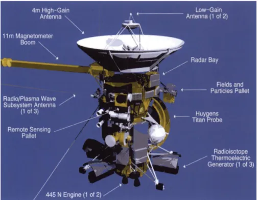
The Cassini-Huygens spacecraft is represented Figure 1.1. It is made of several sections, from top to bottom [29, 44]:
• The High Gain Antenna (HGA)
• The electronic bus, with 12 bays housing the majority of the spacecraft electronics.
• The upper equipment module.
• The propellant tanks with the engines. • The lower equipment module.
Until its release in December 2004 attached on one side there was the three-meter diameter Huygens probe. A 11 m boom supports the Magnetometer (MAG). Three thin 10 m antennas pointing in orthogonal directions are the sensors of the Radio and Plasma Wave Science (RPWS) experiment. Three Radio-isotope Thermal Generators (RTG) provides electrical power through the decaying of an isotope of
1.1. THE CASSINI-HUYGENS MISSION 5
Figure 1.1: The Cassini-Huygens spacecraft in cruise configuration.
Plutonium (Pu-238). The heat generated by this natural process is converted into electrical power by solid-state thermoelectric converters, without any moving part.
Cassini is three-axis stabilized spacecraft. The attitude can be controlled either using the reaction wheels of a set of small thrusters. The instruments are body-fixed, so the observations require to pointing the whole spacecraft. For this reason, during the scientific observations the HGA cannot be used to communicate to the Earth, either for transmit the telemetry or for gravity radio science experiments. The data are recorded on two solid-state recorders (SSR), each of which has a storage capacity of about 2 Gigabits. Due to the effects of solar and cosmic radiation the actual storage capacity decreased with time.
The Cassini-Huygens system carries 18 instruments, 12 on the orbiter Cassini and 6 on the Huygens probe. Most of the orbiter instruments are on two body-fixed platforms, the remote-sensing platform and the particles-and-fields pallet.
A brief description of the Cassini instruments follow [44]:
• Composite Infrared Spectrometer (CIRS): it consists of dual interferometers that measure infrared emission to determine the composition and temperatures of atmospheres, rings, and surfaces.
• Imaging Science Subsystem (ISS): it consists of both a wide angle camera and a narrow angle camera.
• Ultraviolet Imaging Spectrograph (UVIS): the instrument measures the views in ultraviolet spectrum.
• Visual and Infrared Mapping Spectrometer (VIMS): it consists of spectrome-ters observing in visual and infrared spectra.
• Cassini Plasma Spectrometer (CAPS): it measures the flux of ions and elec-trons.
• Cosmic Dust Analyzer (CDA): it measures directly the physical properties of the particles in the Saturn system.
• Ion and Natural Mass Spectrometer (INMS): it measures the composition of neutral and charged particles in Saturn system through mass spectroscopy.
• Dual Technique Magnetometer (MAG): it measures the Saturn magnetic field, its variation with time and interactions with the solar wind.
• Magnetospheric Imaging Instrument (MIMI): it measures the composition, charge state and energy distribution of energetic ions and electrons of the Saturn’s magnetosphere.
• Radio and Plasma Wave Science (RPWS): it measures the electric and mag-netic fields and electron density in the Saturn system.
• Radar (RADAR): it uses the HGA to study the surface composition and properties of bodies of the Saturn’s system. In particular it allows to study the surface of Titan, which is covered by a thick atmosphere layer, opaque in the visible spectrum.
• Radio Science Subsystem (RSS): it studies the compositions of Saturn and Titan atmospheres and ionosphere, the rings structure and the gravity field of Saturn and its satellites.
1.1.4
The Cassini Radio Science Subsystem
In this section the Cassini Radio Science Subsystem will be described in details.
1.1.4.1 Scientific Objectives
During the entire Cassini mission, the following radio science experiments were performed:
• Gravitational Wave Experiments (GWE), to detect the Doppler shift due to low-frequency gravitational waves.
• Solar Conjunction Experiments (SCE), to test the general relativity and study the solar corona.
• Ring occultation experiments.
• Atmospheric and ionospheric occultation experiments, for Saturn and Titan. • Gravitational field experiments, to measure the gravity field of Saturn, Titan
1.1. THE CASSINI-HUYGENS MISSION 7
1.1.4.2 Overview
The radio science instrument is peculiar because it is not confined within the spacecraft, but it is composed by a ground segment and a spacecraft segment, which in turn is distributed among several spacecraft subsystems. Actually, the radio science subsystem can be considered as a solar-system-sized instrument observing at microwave frequencies, with one end a the spacecraft and the other end at DSN station on Earth [28].
The instrument operates in three fundamental modes:
• Two-way mode: the ground station generates one or more uplink signals, at either X-band and Ka-band, using as reference the local frequency and timing system. The signals are amplified, radiated through feed horns and collimated by a large parabolic antenna. The uplink frequency can be constant (unramped) or linearly variable with time (ramped) to compensate for the main Doppler shift due to the spacecraft-station relative motion The spacecraft receives the uplink signals with the High Gain Antenna (HGA), or the Low Gain Antennas (LGA), lock the carrier through the transponder, generates one or more downlink signals that are coherent to the uplink carriers, using the uplink carriers as reference. To prevent interferences, the frequency of the downlink and uplink signals are different. The ratio between downlink and uplink frequqncies is called turn-around ratio. The downlink signal is amplified, collimated and sent back to the earth were it is received, amplified and registered by a ground station. Three types of links can be generated:
– X/X: a X-band downlink signal is generated using the X-band uplink as
reference. The turn around ratio is 880/749.
– X/Ka: a Ka-band downlink signal is generated using the X-band uplink
as reference. The turn around ratio is 3520/749.
– Ka/Ka: a Ka-band downlink signal is generated using the Ka-band
uplink as reference. The turn around ratio is 14/15. At present this link is not available anymore, due to a unrecoverable failure of the KaT transponder.
The use of the three links at the same time allows a complete calibration of dispersive media, like solar plasma and earth ionosphere, using the full multi-frequency link combination [12, 42]. At present, being the KaKa link unavailable, this calibration method cannot be used, limiting the accuracies achievable by the experiments.
• Three-way mode: this mode is the same as two-way mode, but the transmitting and receiving ground station are different. Three-way mode is widely used when the geometric configuration do not allow continuous tracking from the same antenna.
• One-way mode: in this operative mode the source of the signal is the spacecraft. The Ultra-Stable Oscillator (USO) is used as reference to generate one or more downlink signals, at S-, X-, and Ka- bands. These signals are amplified
and radiated through the HGA toward Earth. After passing through the medium of interest (atmosphere, ionosphere, or rings) the perturbed signal is received and recorded by a ground station.
Two-way mode allows to achieve the greatest signal stabilities, because it exploits the greater stability of the ground reference frequency to achieve a signal much more stable. Currently, the DSN frequency standard is based upon a Hydrogen Maser Oscillator, which provides a very accurate frequency reference at the time scales of interest. Typical Allan deviations of the ground clock are of the order of about 10−15 at 1000 s of integration time. As reference, the Allan deviation of the Cassini USO is about 3 × 10⁻¹³ at 1000 s of integration time.
1.1.4.3 Spacecraft Segment
The Radio Science Subsystem is a virtual subsystem composed by the elements from three spacecraft subsystems:
• Radio Frequency Subsystem (RFS).
• Radio Frequency Instrument Subsystem (RFIS). • Spacecraft Antennas.
The Radio Frequency Subsystem The Radio Frequency Subsystem (RFS) is a critical, redundant, spacecraft subsystem which supports spacecraft telecommu-nications, allowing the spacecraft to receive commands and transmit telemetry at X-band. The components of the RFS involved in the RSS are:
• The Ultra-Stable Oscillator (USO). • The Deep-Space Transponders (DSTs).
• The X-band Traveling Wave Tube Amplifiers (X-TWTAs). The RFS has three operative modes:
• Two-way coherent mode: the receiver in the DST locks the uplink carrier, which is used as a reference to generate a coherent downlink signal.
• Two-way non-coherent mode: the uplink carrier is locked into the DST, but the downlink signal is generated using as reference either the USO or the DST auxiliary oscillator.
• One-way mode: in this mode there is no uplink, and a downlink signal is generated using either the USO or the DST auxiliary oscillator.
The DST generates also the input signals for the S-band transmitter (SBT) and the Ka-band exciter (KEX) in the RFIS. Either the USO or the uplink signals can be used.
Cassini’s USO is a crystal oscillator whose internal temperature is maintained constant to within 0.001 K by a proportionally controlled oven. The USO generates
1.1. THE CASSINI-HUYGENS MISSION 9
a 114.9 MHz reference signal with exceptional short-term phase and frequency stability for the DST, SBT, and KEX.
The X-band downlink generated from the DST is amplified by the X-TWTA to 15.8 W, and radiated to Earth through the spacecraft antennas.
The Radio Frequency Instrument Subsystem The elements of the RFIS are devoted exclusively to radio science:
• S-Band Transmitter (SBT): it generates a 13.5 W 2.3 GHz (S-band) carrier from a 115 MHz input signal from the DST. The input signal can derive directly from the USO or can be generated coherently from the uplink signal. The S-band carrier is sent through a diplexer to the HGA.
• Ka-band EXciter (KEX): it generates a Ka-band 32 GHz carrier from both a 115 MHz and a X-band inputs from the DST. These inputs can be generated from the USO (in one-way mode) or coherently from the uplink (in two-way mode). The output is routed through a hybrid coupler to the K-TWTA.
• Ka-band Transponder (KAT): it generates a 32 textGHz downlink signal coherently from a 34 textGHz uplink signal, usign a turnaround ratio of 14/15, with an intrinsic Allan deviation of 3 × 10⁻¹⁵ at 1000 s. integration time. The KAT output goes through the hybrid coupler and then to the K-TWTA.
• Ka-band Traveling Wave Tube Amplifier (K-TWTA): it amplifies the Ka-band output from both the KEX and the KAT, singly or simultaneously, feeding the HGA only. The amplifier produces a total output power of 7.2 W when operating with one carrier and 5.7 W in dual-carrier mode.
The SBT and KAT were fundend by the Italian Space Agency (ASI) and produced by Thales Alenia Space Italy (formerly Alenia Spazio) as part of the Italian participation to the Cassini mission. Alenia Spazio also integrated and tested the RFIS.
Orbiter Antennas Cassini has one High-Gain Antenna (HGA) and two Low-Gain Antennas (LGA1 and LGA2) [63].
• The HGA is Cassegrain system, with a 4 m diameter parabolic primary reflector. The HGA is body-fixed with its boresight along the spacecraft −Z axis and is pointed by moving the spacecraft. In addition to supporting X-band telecommunications, the HGA supports the S-band, X-band and Ka-band radio science links, and serves as the transmit and receive antenna for the Cassini Radar, at Ku-band. It is the most complex antenna ever flown on a planetary spacecraft.
• The LGAs sacrifice gain to provide a relatively uniform coverage. They are used when the HGA can’t be pointed toward the Earth, due to thermal constraints or when the spacecraft is in safe mode. LGA1 is mounted on top of the HGA and points along −Z axis, as the HGA, while LGA2 is
mounted on a boom below the Huygens Probe, and pointing along the −X axis. The LGAs can operate at X-band only. Recently, a test to use LGA for radio science gravity experiments was performed [11]. The test assessed the feasibility to perform precise orbit determination using the LGAs, making it possible to collect data also during satellites fly-bys not dedicated to gravity investigations, at the expense of a small degradation of the signal-to-noise ratio.
Carrier signals transmitted between the spacecraft and the ground are all circularly polarized. X-band uplink and downlink signals can be either Right-hand Circularly Polarized (RCP) or Left-hand Circularly Polarized (LCP). During normal operations the received and transmitted signals have opposite polarizations. The Ka-band uplink is only LCP, and the Ka-band downlink is only RCP.
1.1.4.4 Ground Segment
The ground segment of the Cassini radio science subsystem is composed by the ground stations and facilities of the NASA’s Deep Space Network (DSN). The DSN is composed by three complexes separated in longitude by about 120 deg, to provide a near-global coverage during the diurnal Earth rotation. The complexes are located near Goldstone, in the desert of the Southern California, near Madrid in Spain, and near Canberra in Australia. The first two complexes are in the northern hemisphere, while Canberra is located in the southern hemisphere. Each complex is equipped with several tracking stations of different aperture size and different capabilities, but each complex has at least one 70 m diameter station, one 34 m high-efficiency (HEF) station, and one 34 m beam-wave-guide (BWG) station. While the primary function of the DSN antennas it to send commands and receive telemetry from deep space probes, they are a fundamental part of the radio science instruments, so performances and calibration of the antennas components concur to determine the experiments accuracy. The antennas perform two functions:
• Transmitting function: an uplink signal, at the frequency assigned to the spe-cific spacecraft, is generated using a very stable reference frequency provided by the frequency and timing subsystem. The performance of the frequency and timing subsystem is of order 10−15 for integration times of 1000 s. The uplink frequency can be constant (unramepd) or linearly varying with time (ramped). The DSN can transmit at S-, X- or Ka-bands depending on the transmitting station and the receiving spacecraft. The transmitted frequencies are recorder for post-processing of the two-way Doppler observable.
• Receiving function: the large parabolic primary reflector collect the incoming energy of the spacecraft downlink signals and focus it onto the feed horns. The received signal is amplified through low-noise amplifiers, then it is down-converted and routed to the receivers. These two processes define the most important contribution of the ground segment electronics to the overall noise budget of radio science experiments. Two types of receivers can be used:
– Closed-loop receiver, also called Block V Receiver (BVR): it estimates
1.1. THE CASSINI-HUYGENS MISSION 11
values of receiver bandwidths and time constants. It is the primary DSN receiver for telemetry and tracking data. The signal is phase locked and demodulated from the telemetry and ranging signals. The tracking subsystem measures Doppler shifts and ranging information based on the closed-loop receiver output.
– Open-loop receiver, also called Radio Science Receiver (RSR): it record
the electric field of the received signal downconverting and digitizing a selected bandwidth of the spectrum centered around the carrier signal. The RSR had several advantages with respect to the BVR:
∗ More flexibility because the data (amplitudes and phases) are com-puted in post-processing.
∗ Better performances due to more stringent requirements on ampli-tude, frequency and phase noise stability.
∗ Simultaneous handling of signals in two polarization states.
Media Calibration System The Earth’s troposphere is one of the most relevant noise contribution to the overall noise budget of the orbit determination process [9, 27, 34]. The neutral particles of the atmosphere introduce a phase and a group delay in the signal. The main contribution is represented by the gases in the lower part of the atmosphere, in particular the water vapor. Being a non-dispersive media, the group and phase delay are the same. In order to provide a continuous troposphere calibration a system based on GPS observation has been developed by JPL. The system, named Tracking System Analysis Calibration (TSAC) uses the GIPSY-OASIS II software to create continuous calibration of the Zenith Total Delay (ZTD). The delay along the line of sight of the spacecraft is obtaining scaling the ZTD with mapping functions.
In order to achieve the unprecedented accuracies needed by the Cassini’s cruise radio science experiments, a new generation of media calibration system, called Advanced Media Calibration system (AMC), was developed [10, 52, 57, 58]. The AMC includes different meteorological instruments to retrieve the entire troposphere delay:
• A high-stability Water Vapor Radiometer (WVR), which senses the number of water vapor molecules along the line of sight.
• A Microwave Temperature Profiler (MTP), which senses the vertical temper-ature distribution.
• A Surface Meteorological station (SM), which measures the temperature, pressure and humidity.
The AMC system provides the most accurate calibration of the tropospheric noise to date, because it is capable to measure with very good accuracy the high-frequency scintillations of the tropospheric path delay due to variation of water vapor content along the line of sight.
1.2
The Orbit Determination Problem
1.2.1
Introduction
This Section provides a high-level description of the procedures to be imple-mented in order to correctly analyze Doppler data acquired during gravity radio science experiments on interplanetary missions. This analysis is strictly linked to the problem of orbit determination of interplanetary spacecraft. The orbit deter-mination process is an iterative estimation procedure based upon the comparison between the measured observables (observed observables) and the corresponding computed values (computed observables), computed on the basis of mathematical models. The difference between the observed and the computed observables are called residuals. The aim of the orbit determination process is the estimation of a set of parameters (solve-for parameters) that unambiguously define the trajectory of a spacecraft. The orbit determination solution is composed by the value of the solve-for parameters that minimizes, in a least square sense, the residuals, and by the corresponding covariance matrix that defines the formal uncertainty of the solution. For Deep Space navigation purposes, the orbit determination S/W is typically used to analyze large data sets and estimate a large number of solve-for parameters, with the aim of providing the best estimate of the S/C state, for the need of both S/C operations and scientific data analysis. On the other hand, for radio science applications, typically small data sets acquired during the limited time intervals of dedicated experiments are analyzed in the orbit determination S/W, aiming at the estimation of a restricted set of parameters (in addition to the S/C state vector) that defines the gravity field of celestial bodies. These experiments are carefully designed in order to minimize the uncertainties in the orbit determination process and to maximize the Signal to Noise Ratio of the solve-for parameters. For gravity radio science experiments the solve-for parameters may include:
• coefficients of the gravity spherical harmonics expansion of a celestial body; • Love’s numbers, the define the gravity field response to external tidal effects; • Rotational parameters of a celestial body.
The gravity field, and so the gravitational acceleration of the spacecraft, are a consequence of the planet/satellite internal composition and mass distribution, so the experiments results can be used to develop and test models of the origin, evolution and structure of celestial bodies, like planets, satellites and asteroids. Moreover the experiments can be used to test the general relativity, measuring relativistic effects like the Shapiro light-time delay or the Lense-Thirring effect.
The orbit determination process can be divided into five main steps:
• Pre-processing of radiometric measurements.
• Computation of radiometric observables and partial derivatives with respect to the solve-for parameters, using mathematical models.
1.2. THE ORBIT DETERMINATION PROBLEM 13
• Estimation filter. • Solution analysis.
Because of the intrinsic non-linearity of the problem, these steps are usually repeated until convergence is reached. In the first iteration the observables and partials are computed using apriori values of the solve-for parameters. The estimation filter computes differential corrections to these values, on the basis of comparison between computed and observed observables. In the next iterations the observables are computed using the solution of the previous iteration for the solve-for parameters.
In the following each of these steps will be described from an operational point of view. For more details about the modelization of all the physical effects, see [51] and [54].
1.2.2
Pre-processing of radiometric measurements
During the pre-processing phase the radiometric observables are prepared for the orbit determination process. The most important Earth-based radiometric observables are:
• range: measured round-trip light time, in range units.
• Doppler: frequency shift of the carrier of the received signal.
• DDOR: angular measurement of the S/C along a baseline formed by two ground stations.
On these data, one or more of the following actions may be performed before the analysis:
• Apply the calibrations to correct intrinsically not predictable effects that could affect the measurements, like:
– group delay due to electronics in ground stations and spacecraft; – group and phase delay due to propagation media, like troposphere,
ionosphere and interplanetary plasma;
The calibrations are computed and provided by JPL.
• Compute received sky frequencies from open-loop recordings.
• Compute synthetic non-dispersive observables, if a multi-frequency link is available.
• Delete macroscopic invalid data (outliers). Typically up to 20% of the data may be removed in this phase.
1.2.3
Observables and partials computation
During this phase, the radiometric measurements are simulated using math-ematical models of all physical effects that affect, in a not-negligible way, their values. The parameters that define the mathematical models can be divided into three categories:
• Solve-for parameters: not exactly known parameters that affect data and whose current estimate can be improved through the orbit determination process. At the first iteration their a priori values and uncertainty are used, obtained from the best measurements or theoretical estimations available to date. In the next iterations the solution obtained at the previous iteration is used. The solve-for parameters should always include the initial state of the spacecraft.
• Consider parameters: not exactly known parameters that affect data and whose current estimate cannot be improved through the analysis. Their best estimate to date must be used in the mathematical models, together with their uncertainties. The orbit determination filter does not change the consider parameters, but their uncertainty increases the solution covariance matrix.
• Exact parameters: parameters that are theoretically exactly known or whose uncertainty does not affect the estimation, because it is small with respect to their influence on measurements data.
Moreover, during this phase, also the partial derivatives of the observables with respect to the solve-for and consider parameters are computed. They are used to obtain the new estimate of the value of solve-for parameters and their covariance matrix.
The observables and partials computation is performed through the following procedures:
• Planetary and/or Satellite ephemerides update;
• Integration of equations of motion and variational equations; • Time transformations;
• Ground Station state computation; • Light-time solution computation;
1.2.3.1 Planetary and/or Satellite ephemerides update
The spacecraft trajectory and the radiometric measurements depend on the gravity fields of nearby celestial bodies and relative positions between the spacecraft and celestial bodies. Hence, depending on the type of radiometric observables and geometry of the observation, to correctly extract the information content from the measurements should be necessary to estimate also the planetary and/or satellite ephemerides. For example, during gravity radio science experiments of
1.2. THE ORBIT DETERMINATION PROBLEM 15
planetary satellites, the spacecraft trajectory and so the Doppler data are affected in a not-negligible way by the gravitational fields of both the planet and the satellite. So, the measurements are sensitive to the relative positions and velocities of the spacecraft, the satellite, and the planet. Hence, the orbit determination fit shall estimate both the planetary state of the spacecraft and of the satellite. As another example, the orbit of Mercury is heavily affected by relativistic effects. Accurate range measurements from a Mercury orbiter can be used to test the validity of the Einstein’s general relativity, for example through the estimation of the Parameterized Post-Newtonian parameters γ and β. This requires the capability to update the planetary ephemerides of Mercury. At the first iteration of the orbit determination process the most updated ephemeris available at date are used, while in the next iterations the ephemerides should be updated using the estimate of the previous iteration. Ephemerides are generated integrating the full relativistic equations of motion of the planets from their initial states. The partials needed to update the ephemerides are obtained integrating the variational equations for the planetary/satellite state.
1.2.3.2 Integration of equations of motion and variational equations
The next step to compute the radiometric observables and partials is to recon-struct the spacecraft trajectory integrating the equations of motion with respect to a reference point (Center Of Integration, COI) from an input initial state. The a priori value (and uncertainty) of the initial state is usually given by the mission navigation team. To correctly reconstruct the spacecraft trajectory all non-negligible accelerations acting on the spacecraft and on the COI must be correctly modeled. The most important accelerations that may influence the spacecraft state are:
• Point-mass Newtonian gravitational acceleration due to the Sun, the planets, Pluto, small bodies, as asteroids and comets, the Moon and all satellites of a planetary system.
• Point-mass relativistic perturbative gravitational acceleration due to the Sun, the planets, Pluto and the Moon.
• Acceleration due to Geodesic precession. • Acceleration due to Lense-Thirring precession.
• Newtonian acceleration due to the gravitational spherical harmonics of all the planets, Pluto, small bodies, as asteroids and comets, the Moon and all satellites of a planetary system. The acceleration of the S/C relative to the COI due to oblateness of one of the bodies listed above is computed as the acceleration of the S/C (direct component) minus the acceleration of the COI (indirect component). If also the COI is an oblate body, the acceleration of
the COI is the sum of two terms:
– the acceleration due to the spherical harmonics of the oblate body on
– the acceleration due to the point-mass oblate body on the COI’s
oblate-ness.
The acceleration due to the interaction between the oblateness of the body and the COI is neglected.
• Relativistic acceleration due to the gravitational spherical harmonics: this effect is usually considered only for the Earth’s gravity field on a near-Earth S/C.
• Accelerations caused by tidal effects on the physical central body: the accel-eration of the S/C derives from corrections to the central body’s normalized harmonic coefficients due to the tides as:
– solid tides; – ocean loadings; – pole tides.
• Gravitational acceleration due to planetary rings. • Gravitational acceleration due to mascons.
• Solar radiation pressure;
• Planetary radiation pressure: acceleration due to the radiation emitted from the surface of a planet, both reflected visible light (albedo) and thermal emission.
• Thermal imbalance: acceleration due to non-uniform surface heating. • Gas leakage: acceleration due to control jets leakage.
• Atmospheric drag. • Maneuvers.
To compute the various contributions to the total spacecraft acceleration the position of the celestial bodies must be known, through planetary, satellite and small bodies ephemerides. At present the most accurate celestial ephemerides are provided by NASA/JPL, eventually updated in the previous step of the orbit determination process.
1.2.3.3 Time transformations
All radiometric observables measured at different tracking stations on the Earth are referred to the time measured by the station clock. Apart from a small drift due to clock stability, the station reference time is equal to UTC. However, to correctly compute the light-time solution, time must be expressed in Barycentric Coordinate Time (TCB), the coordinate time of the relativistic equations of motion in the Solar
1.2. THE ORBIT DETERMINATION PROBLEM 17
System barycentric space-time frame of reference or in a linear transformation of TCB, like JPL Ephemeris Time (Teph) or Barycentric Dynamical Time (TDB)1.
1.2.3.4 Ground station state computation
The location of a ground station is conventionally defined as the position of a reference point. The station’s coordinates are given as inputs in a terrestrial reference frame, then the station location must be corrected to account for various effects:
• Solid Earth tides: the tides caused by the Moon and the Sun produce deformations of the Earth that change the location of the ground station. At least first order displacements and second order corrections due to a tidal potential of degree two due to both the Moon and the Sun must be considered. The first order displacement is about 50 cm, while the second order correction is about 13 mm. Usually the permanent tidal displacement is included in the expression of the first-order displacement, so the coordinates of the tracking stations must not include it. At present, terms less than 5 mm can be neglected.
• Ocean loadings: periodic displacements due to the periodic ocean tides. The displacements are less than 4 mm.
• Pole tide: the polar motion modifies the centrifugal potential of the Earth and caused a solid tide that produces a displacement of the tracking station. The displacement is less than 2 cm.
• Plate motion: a tracking station has a non zero velocity due to the tectonic plate motion. The station velocity due to plate motion can be up to 10 cm/y.
• Offset between the real COM of the Earth and the origin of the considered terrestrial reference frame.
Next, in order to solve the light-time problem it is necessary to convert the station location from the terrestrial reference frame to the celestial reference frame. The transformation between the two reference frames consists of a series of rotations:
• polar motion; • Earth rotation; • nutation; • precession.
1Since JPL’s DE430, the Ephemeris Time T
eph coincides with Barycentric Dynamical Time
TDB, that is a defined linear transformation of TCB. For the older ephemerides Teph is formally
different from TDB, because it was computed as a part of the ephemerides estimation to remove a linear drift with the Terrestrial Time (TT). However, this difference at present is completely negligible.
These rotations are defined by a set of parameters, that depend on the particular modelization selected. An internal group at NASA/JPL provides the so-called Earth Orientation Parameters (EOP), that define these rotations according to IAU 1980 Theory of nutation and the IAU 1976 Precession Model. As an alternative, the more accurate IAU 2000 Model can be used. The coefficients defining the rotations are provided either by JPL or by IERS website2. After these rotations the
geocentric state of the tracking station is expressed in the Geocentric space-time frame of reference, and it must be referred to Solar System barycentric space-time frame of reference, through proper Lorentz transformations.
1.2.3.5 Light-time solution computation
The next step to evaluate the computed value of a measured quantity is to obtain the solution of the light-time problem for that observable. The light-time solution consists of the epoch of participation and the state of each direct participant at its epoch of participation. The direct participants of the light-time problem and the times of participation are:
• the receiving station at the reception time t3;
• the S/C at the reflection time (for two-way or three-way observables) or transmission time (for one-way observables) t2;
• the transmitting station at the transmission time t1 (only for two-way or
three-way observables).
In the orbit determination process, the reception time of an observed quantity is known, so it is necessary to solve the light-time problem to compute the reflection time and the transmission time. The light-time problem is based upon the expression of the time for light to travel from the transmitter to a receiver. This time is the sum of two components:
• Newtonian light-time, that represents the time for light to travel along a straight-line path at the speed of light c.
• The relativistic light-time delay, also called Shapiro effect, that accounts for the reduction of the coordinate velocity of light below c and the bending of the light path due to presence of a gravity field that curves the space-time.
1.2.3.6 Observables computation
The outputs of the light-time problem are used to compute the value of ra-diometric observables measured at Earth tracking stations. Moreover, the partial derivatives of the observables with respect to the solve-for parameters are computed. The model of the radiometric observables obtained at the stations of the Deep Station Network (DSN) and the corresponding partials are described in [51].
1.2. THE ORBIT DETERMINATION PROBLEM 19
1.2.4
Estimation Filter
The estimation filter computes the value of the solve-for parameters that mini-mize, in a least square sense, a combination of the following quantities:
• Residuals between the observed and computed observables. The residuals should be weighted with their measurements noise. However, because noise is not known, as a start to the analysis an a-priori value is used, on the basis of available theoretical error budgets or experience. In the next analysis the measurements noise is estimated as the residuals’ standard deviation. Note that this imply the assumption that the measurements noise is white. In the different iterations of the same analysis residuals weights are kept constants.
• Difference between the solve-for parameters and their a priori values. This difference is weighted using the uncertainty of the a-priori information. From a filtering point of view, a priori data are equivalent to additional observations. They are used to increase the numerical stability of the information matrix and facilitate the convergence.
The estimation filter produces two outputs:
• A differential correction to a priori values of the solve-for parameters. It gives the updated estimate of the solve-for parameters.
• The covariance matrix of the solve-for parameters, that represents the solution uncertainty. The a priori covariance matrix is updated on the basis of the influence on the solve-for parameters of the measurements noise and consider parameters uncertainty.
1.2.5
Solution Analysis
The solution obtained from the estimation filter should be verified and tested. The following aspects should be analyzed:
• Convergence: the orbit determination process reaches convergence if two (or more) successive iteration steps produce statistically equivalent solutions.
• Residuals analysis: the obtained solution is used to compute residuals. If the orbit determination process was performed correctly solution residuals represent only measurements noise, hence they must verify the following conditions:
– Zero mean: the residuals mean must be much less than their standard
deviation, i.e. compatible with a zero value;
– Spectrum compatible with the expected noise characteristics;
Moreover, the residuals standard deviation should be compatible with the residuals weight used in the estimation filter.
– Comparison between a priori and computed formal uncertainties: a
parameter is fully observable from data if the computed uncertainties are much less than the a priori ones (as reference a factor 10 can be used). Otherwise, the estimation depends much more on a priori information than on radiometric measurements.
– Cross-correlation between solve-for parameters: if two solve-for
parame-ters are largely correlated, their estimation is strictly dependent.
• Comparison between a priori values and the new estimates: the new and old estimate of the solve-for parameters should be statistically compatible.
• Solution stability: to check the solution stability it is useful to make another estimation process using the solution as a priori values, with ”relaxed“ in-creased a priori uncertainties. If the solution is sufficiently stable the new estimation will be statistically compatible with the testing solution.