Neural network approach to problems of static/dynamic classification

(1)

UNIVERSITY OF ROME

“TOR VERGATA”

Faculty of Engineering

Ph. D. Thesis on Engineering of Sensory and Learning Systems:

“N

eural network approach to Problems of

Static/Dynamic Classification”

Supervisor

Assistant

Supervisor

Prof. Mario Salerno

Ing. Giovanni Costantini

Ph. D. Student

Ing. Massimo Carota

Winter Session Academic year 2006/2007

(2)

Abbreviations and symbols

M

n° of layers in the network

l

layer index. l = 0 ⇒ input layer, l = M ⇒ output layer

N

_l # of neurons in the lth layer. N0 = # of inputs, NM = # of outputs

n

neuron index

T

length of an input sequence (length of a learning epoch)

t

time index: t=1,2 ,_K,T ( )

[ ]

t

x_nl nth neuron output sequence in the lth layer at time t. x₀( )l =1 : bias input to next layer. x( )_n0

[ ]

t

, n=1,_K,N₀ : input signals supplied to the network. ( )

1 −

l

nm

L In a IIR-MLP, it’s the order of the MA part of the synapse of the nth neuron of the lth layer relative to the mth output of the (l - 1)th layer. L( )nml ≥1 and

( ) 1 0 = l n L (bias). ( )l nm

I In a IIR-MLP, it’s the order of the AR part of the synapse of the nth neuron of the lth layer relative to the mth output of the (l - 1)th layer. Inm( )l ≥0 and

( ) 0 0 = l n I (bias). ( )l nm

w static MLP: weights of the nth neuron (n=0,K,Nl−1) in the l

th

layer (l =1,_K,M ), mth neuron output from the previous layer (m=0,_K,N_l₋₁); w_n( )l₀ is the bias.

( )

( )l

p nm

w

(

p=0 ,1 ,_K ,L( )_nml −1

)

In a IIR-MLP, are the coefficients of the MA part of the corresponding synapse. If , L( )_nml =1, the synapse has no MA part and the weight notation becomes w . nm( )l ( )l n w0 is the bias. ( ) ( )l p nm

v

(

p=1 ,_K ,I_nm( )l

)

In a IIR-MLP, are the coefficients of the AR part of the corresponding synapse. If I_nm( )l =0, the synaptic filter is purely MA.

υ

_w

_or

_v

_coefficient

( )

• ϕ activation function

( )

• ′ ϕ derivative of ϕ

( )

• ( )

_{[ ]}

t

y_nml In a IIR-MLP, it’s the synaptic filter output at time t relative to the synapse of nth neuron, of the lth layer, and the mth input. y_n( )l₀ =w_n( )l₀is the bias.

( )

_{[ ]}

t

s_nl activation sequence relative to the nth neuron, of the lth layer, at time t. It’s the input to the corresponding activation function.

[ ]

t

d_n

(

n=1,K,NM

)

desired output sequence at time

t

.

N + 1

spline activation function: # of control points

x

∆ spline activation function: abscissa sampling step ( )l

n

i spline activation function: (0≤i_n( )l ≤ N−2) nth neuron, lth layer, index of the curve span

( )l

n

u spline activation function: (0≤un( )l ≤1) n

th

neuron, lth layer, local parameter for the curve span

( )l k n

q _, spline activation function: (0≤k≤ N) nth neuron, lth layer, ordinate of the kth

control point ( ) ( )l

_{( )}

_• l n i n F

, spline activation function: n

th

neuron, lth layer, mth CR polynomial ( )l

_{( )}

_•

m n

(9)

P

REFACE

The purpose of my doctorate work has consisted in the exploration of the potentialities and of the effectiveness of different neural classifiers, by experimenting their application in the solution of classification problems occurring in the fields of interest typical of the research group of the “Laboratorio Circuiti” at the Department of Electronic Engineering in Tor Vergata.

Moreover, though inspired by works already developed by other scholars, the adopted neural classifiers have been partially modified, in order to add to them interesting peculiarities not present in the original versions, as well as to adapt them to the applications of interest.

These applications can be grouped in two great families. As regards the first application, the objects to be classified are identified by features of static nature, while as regars the second family, the objects to be classified are identified by features evolving in time. In relation to the research fields taken as reference, the ones that belong to the first family are the following:

• classification, by means of fuzzy algorithms, of acoustic signals, with the aim of attributing them to the source that generated them (recognition of musical instruments)

• exclusive classification of simple human motor acts for the purpose of a precocious diagnosis of nervous system diseases

The second family of application has been represented by that research field that aims to the development of neural tools for the Automatic Tanscription of piano pieces.

The first part of this thesis has been devoted to the detailed description of the adopted neural classification techniques, as well as of the modifications introduced in order to improve their behavior in relation to the particular applications. In the second part, the experiments by means of which I have estimated the before-mentioned neural classification techniques have been introduced.

(10)

It exactly deals with experiments carried out in the chosen research fields. For every application, the results achieved have been reported; in some cases, the further steps to perform have also been proposed.

After a brief introduction to the biological neural model, a description follows about the model of the artificial neuron that has afterwards inspired all the other models: the one proposed by McCulloch and Pitts in 1943. Subsequently, the different typologies of architectures that characterize neural networks are shortly introduced, as regards the feed-forward networks as well as the recursive networks. Then, a description of some learning strategies (supervised and unsupervised), adopted in order to train neural networks, is also given; some criteria by means of which one can estimate the goodness of an opportunely trained neural network are also given (errors made vs. generalization capability). A great part of the adopted networks is based on adaptations of the Backpropagation algorithm; the other networks have been instead trained by means of algorithms based on statistical or geometric criteria. The Backpropagation algorithm has been improved by augmenting the degrees of freedom to the learning ability of a feed-forward neural network with the introduction of a spline adaptive activation function. A wide description has been given of the recurrent neural networks and particularly of the locally recurrent neural networks, networks for dynamic classification exploited in the automatic transcription of piano music.

After a more or less rigorous definition of the concepts of classification and clustering, some paragraphs have been devoted to some statistical and geometric neural architectures, exploited in the implementation of static classifiers of common use and in particular in the application fields that have regarded my doctorate work.

A separate paragraph has been devoted to the Simpson’s classifier and to the variants originated from my research work. They have revealed themselves to be static classifiers very simple to implement and at the same time very ductile and efficient, in many situations as well as regards the

(11)

problem of musical source recognition. Two have been the choices in this case. In the first one, these classifiers have been trained, by means of a pure supervised learning approach, while in the second the training algorithm, though keeping a substantially supervised nature, is prepared by a clustering phase, with the aim of improving, in terms of errors and generalization, the covering of the input space. Subsequently, the locally recurrent neural networks seen as dynamic classifiers are retrieved. However, their training has been rethought according to the effective reduction of the classification error instead of the classic mean-square error.

The last three paragraphs have been devoted to a detailed description, in terms of specifications, implementative choices and final results, of the aforesaid fields of applications. The results obtained in all the three fields of application can be considered encouraging. Particularly, the recognition of musical instruments by means of the adopted neural networks has shown results tha can be considered out comparable if not better than those obtained by means of other techniques, but with considerably less complex structures. In case of the Automatic Transcription of piano pieces, the dynamic networks I adopted have given good results. Unfortunately, the required computational resources required by such networks cannot be considered negligible. As far as the medical applications, we are still in an incipent phase of the research. However, opinions expressed by those people who work in this field can be considered substantially eulogistic.

The research activities my doctorate work is part of have been carried out in collaboration with the Department “INFOCOM” of the first University of Rome “La Sapienza”, as far as the recognition of musical instruments and the Automatic Transcription of piano pieces. The necessity to study the potentialities of neural classifiers in medical application has instead come from a profitable existing collaboration with the Istituto Superiore di Sanità in Rome.

(12)

I

NTRODUCTION

Given some set of whatever kind of objects (called patterns), the classification process is essentially based on the peculiar traits and/or mutual relationships existing among those objects, that lie behind the structure of that set and that allow the identification of significant subsets, called classes. Each one of these classes includes objects that share, so to speak, the same “values” of those traits, or, in other words, that that are in some relation among each other. The detection of the above mentioned structure is carried out by means of an abstraction process, that, for every class, leads to the definition of a “model” representing all the objects belonging to that class, as regards only the relevant peculiarities of its objects. On the contrary, the “model” has to necessarily set aside all the characteristics of the objects that can be somehow considered not essential. The more this “model” is accurate, the more it will be effective when used to associate a new object to the class to which this object belongs to. These concepts can be better clarified by the following example. Every people is more or less aware of what a car can be, that is to say, of what the common “idea” (the “model”) of a car can be. If we face a collection of many sorts of objects, we will most probably be capable of identifying among them one or more objects that we can call “a car”.

The identification process can be briefly summarized, as follows:

1. every object in the collection is compared with the personal “idea” of a car, an “idea” based on the experience previously acquired about

2. each object is labelled as being a car, or less, depending on its adherence to the model

Obviously, some characteristics, as for example the colour of the car, are not relevant in order to the classification process; thus, we shouldn’t find any sign of it inside the abstract model of a car. On the contrary, the model should include information about the salient characteristics distinguishing a car from any other object, as for example: a car has four wheels, some doors, as well as proper dimensions and mass. The key to the successful solution of a classification problem consists mainly in the correct development of the above mentioned descriptive models. A problem strictly related to classification is clustering. Trivially speaking, in classification the knowledge about number and type of classes is previously given, while clustering is a process that aims to discover the presence of agglomerates of objects, identified by having common characteristics, inside a universe of them, agglomerates that can be subsequently named classes. In other words, in classification the structure of the universe is known in advance, while in clustering it must be identified by clustering operation itself. The first obstacle to overcome, in the design of an automatic classification and/or

(13)

clustering system, regards the correct method to adopt in creating the “model” that embeds the characteristics of the different classes involved.

A first approach can be the analytical one, according to which the designer incorporates his knowledge about the application at issue into the elaboration system, in the form of an algorithm, i.e. a set of rules that the system has to slavishly follow when it is asked to face up to that application. Particularly, this is the approach followed by a programmer, when he develops a program that implements a simulation algorithm, in one of the existing programming languages. Nevertheless, this strategy has many drawbacks. First of all, the resulting elaboration system would have potentialities and knowledge at most coincident with those of its creator; it would be rigorously static, that is, it would be structurally unable to “grow up”. Moreover, the system would be unable to tackle situations that the designer was previously unable to foresee, or that cannot be faced starting from the instructions that the designer gave to it (induction inability). Furthermore, every problem to solve would require a well defined system typology, to be designed from scratch whenever a new application is proposed (system architecture strictly bounded to the problem). Last but not least, some problems would require calculation systems with a so high degree of complexity that every practical implementation would be inconceivable.

Anyway, we can imagine to turn to a radically different approach. If we take a look at how human brain constructs its mental categories, we jump to the following deduction: a classification system has to be able to “learn”, that is to say, to build by itself (in an unsupervised way) abstract models, on the basis of examples (the learning or training process). Moreover, it must be provided with some kind of reasoning ability, thru which it can handle even situations that it never faced before (generalization capability, or validation). In some sense, this will be the approach that we will follow. Precisely, to efficiently solve problems of classification ad clusterization we will turn to a computational paradigm directly inspired to human brain: neural networks.

Neural networks are particularly suited to problems of classification ad clusterization thanks to their generalization capabilities. Actually, and according to what we stated before, the solution of a classification problem cannot be accomplished regerdless this capability. An important challenge in classification consists in extending some of the standard algorithms from simple static data (this is the situation until now considered, actually), to time varying data. In fact, it will be essential for our purposes to extend classification algorithms from data sets consisting of static vectors (points) to data sets consisting of time varying vectors (trajectories), in order to face problems of dynamic classification, based on some form of time series processing. We will consider the special case in which time varying data are collected by sampling trajectories from an underlying family of parameterized dynamical systems. Dynamic classification problems occur frequently in practice:

(14)

• time series prediction and modelling • noise cancelling

• adaptive equalization of a communication channel • adaptive control

• system identification

In order to describe, explore and control the behaviour of linear systems, dynamical system theory provides us with a very efficient tool, but it reduces to a local analysis tool when the hypothesis of linearity falls. Unfortunately, most of the classification problems are non linear. So, for this reason also, neural networks are an essential tool.

(15)

C

HAPTER

1

NEURAL

NETWORKS

1.1 The Brain, the nervous system and their model

Learning is a mental process by means of which experience influences human behaviour. At the foundation of this process, we can find an extremely complex structure: the brain. Much as been discovered about the real working of human brain, but a lot still remains to be explained. Anyhow, medical researches have established many of the processes that occur inside of it. Human brain is essentially a huge and highly complex network in the nodes of which we can find the so called nerve cells, or neurons. Human brain contains about 10 billion neurons. On average, each neuron is connected to other neurons through about 10000 synapses. The brain’s network of neurons forms a massively parallel information processing system. This contrasts with conventional computers, in which a single processor executes one or more series of instructions. Just for comparison, let’s consider the time taken for each elementary operation: neurons typically operate at a maximum rate of about 100 Hz, while a conventional CPU carries out several hundred million machine level operations per second. Nevertheless, despite of being built with very slow hardware, the brain has quite remarkable capabilities:

• In case of partial damage, its performances tend to degrade a little. In contrast, most programs and engineered systems are very little robust: if you remove some arbitrary parts, very likely the whole will cease to function.

• it can learn (reorganize itself) from experience.

• this is why partial recovery from damage is possible: healthy units can learn to take over the functions previously carried out by the damaged areas.

• it performs massively parallel computations with extreme efficiency. For example, complex visual perception occurs within less than 100 ms!

• it supports our intelligence and self-awareness (but nobody still knows how this occurs) The brain is not homogeneous. At the largest anatomical scale, we distinguish cortex, midbrain, brainstem, and cerebellum. Each of these can be hierarchically subdivided into many regions and areas within each region, either according to the anatomical structure of the neural networks that form them or according to the functions they perform (Fig 1.1).

(16)

Fig. 1.1. the brain.

The overall pattern of projections (bundles of neural connections) between areas is extremely complex, and only partially known. The best mapped (and largest) system in the human brain is the visual system, where the first 10 or 11 processing stages have been identified. We distinguish feedforward projections that go from earlier processing stages (near the sensory input) to later ones (near the motor output), from feedback connections that go in the opposite direction. In addition to these long-range connections, neurons also link up with many thousands of their neighbours. In this sense they form very dense, complex local networks (Fig 1.2).

Fig. 1.2. the neural network.

1.1.1 The Biological Neuron

The basic computational unit in the nervous system is the nerve cell, or neuron. It’s formed by: • Dendrites (inputs)

• Cell body

• Axon (output)

A neuron (Fig. 1.3) has a roughly spherical cell body called soma. Signals generated in the soma are transmitted to other neurons through an extension on the cell body called axon, or nerve fibre. Around the cell body, we can find other extensions, called dendrites (bushy tree shaped), which are responsible for receiving the incoming signals generated by other neurons. The axon (Fig. 1.3), has a length that varies from a fraction of a millimetre to a meter in human body and prolongs from the cell body at the point called axon hillock. At the other end, the axon splits into several branches, at the very end of which we find the terminal buttons. Terminal buttons are placed in special structures called the synapses which are the junctions transmitting signals from one neuron to

(17)

another. A neuron typically drives 103 to 104 synaptic junctions.

Fig. 1.3. the biological neuron.

A neuron’s dendritic tree is connected to a thousand neighbouring neurons; so, a neuron receives its input from other neurons (typically many thousands). When one of those neurons fires, a positive or negative charge is received by one of the dendrites. The strengths of all the received charges are added together and the aggregate input is then passed to the soma (cell body). The soma and the enclosed nucleus don’t play a significant role in the processing of incoming and outgoing data. Their primary function is to perform the continuous maintenance required to keep the neuron functionalities. The part of the soma that participates to the elaboration of the incoming signals is the axon hillock: if the aggregate input is higher than the axon hillock’s threshold value, then the neuron fires (the neuron becomes active, otherwise it remains inactive) and an output signal is transmitted down the axon. In other words, once input exceeds the threshold, the neuron discharges a spike – an electrical pulse that travels from the body, down the axon, to the next neuron(s) (or other receptors). This spiking event is also called depolarization and is followed by a refractory period, during which the neuron is unable to fire. The terminal buttons (output zones) almost touch the dendrites or cell body of other neurons, leaving a small gap. Transmission of an electrical signal from one neuron to another is effected by neurotransmitters, chemicals transmitters which are released from the first neuron and which bind to receptors in the second. This link is called a synapse (Fig. 1.4). The synaptic vesicles, holding several thousands of molecules of neurotransmitters, are situated in the terminal buttons. When a nerve impulse arrives at the synapse, some of these neurotransmitters are discharged into the synaptic cleft – the narrow gap between the terminal button of the transmitting neuron and the membrane of the receiving neuron. In general, the synapses lie between an axon branch of a neuron and the dendrite of another neuron. Although it is not very common, synapses may also lie between two axons or two dendrites of different cells or between an axon and a cell body. Neurons are covered with a semi-permeable 5 nm membrane, that’s able to selectively absorb and reject ions in the intracellular fluid. The membrane basically acts as an ion pump in order to maintain a different ion concentration between the intracellular fluid and extra cellular fluid. While the sodium ions are continually removed from the intracellular fluid to extra cellular fluid, the potassium ions are absorbed from the extra cellular fluid in order to

(18)

maintain an equilibrium condition.

Fig. 1.4. the synapse.

Due to the difference in the ion concentrations inside and outside, the cell membrane become polarized. In equilibrium, the interior of the cell is observed to be 70 mV (resting potential) negative with respect to the outside of the cell. Nerve signals arriving at the presynaptic cell membrane cause neurotransmitters to be released in to the synaptic cleft; then they diffuse across the gap and join the postsynaptic membrane of the receptor site. The membrane of the postsynaptic cell gathers the neurotransmitters. This cause either a decrease or an increase in the efficiency of the local sodium and potassium pumps, depending on the type of the chemicals released in the synaptic cleft. The synapses whose activation decreases the efficiency of the pumps cause depolarization of the resting potential, while the synapses which increases the efficiency of pumps cause its hyper polarization. The first kind of synapses (encouraging depolarization) is called excitatory, while the others (discouraging depolarization) are called inhibitory. If the decrease in the polarization is adequate to exceed a threshold then the post-synaptic neuron fires. The arrival of impulses to excitatory synapses adds to the depolarization of soma, while inhibitory effect tends to cancel out the depolarizing effect of excitatory impulse. In general, although the depolarization due to a single synapse is not enough to fire the neuron, if some other areas of the membrane are depolarized at the same time by the arrival of nerve impulses through other synapses, it may be adequate to exceed the threshold and fire. The excitatory effects result in interruption of the regular ion transportation through the cell membrane, so that the ionic concentrations immediately begin to equalize as ions diffuse through the membrane. If the depolarization is large enough, the membrane potential eventually collapses, and for a short period of time the internal potential becomes positive (Fig. 1.5). The action potential is the name of this brief reversal in the potential, which results in an electric current flowing from the region at action potential to an adjacent region with a resting potential. This current causes the potential of the next resting region to change, so the effect propagates in this manner along the membrane wall. Once an action potential has passed a given point, it cannot be re-excited for a short period of time called refractory period. Because the depolarized parts of the neuron are in a state of recovery and cannot immediately become active again, the pulse of electrical activity propagates forward only.

(19)

Fig. 1.5. The Action Potential on Axon.

The previously triggered region then rapidly recovers to the polarized resting state, due to the action of the sodium potassium pumps. The refractory period is about 1000 ms, and it limits the nerve pulse transmission, so that a neuron can typically fire and generate nerve pulses at a rate up to 1000 pulses per second. The number of impulses and the speed at which they arrive at the synaptic junctions determine whether the total excitatory depolarization is sufficient to cause the neuron to fire and send a nerve impulse down to its axon. The depolarization effect can propagate along the cell wall but these effects can be dissipated before they reach the axon. However, once the nerve impulse reaches the axon hillock, it will propagate until it reaches the synapses where the depolarization effect will cause the release of neurotransmitters into the synaptic cleft. The axons are generally enclosed by myelin sheath. The speed of propagation down the axon depends on the thickness of the myelin sheath that provides for the insulation of the axon from the extra cellular fluid and prevents the transmission of ions across the membrane. The myelin sheath is interrupted at regular intervals by narrow gaps called nodes of Ranvier, where extra cellular fluid comes into contact with membrane and the transfer of ions occur. Since the axons themselves are poor conductors, the action potential is transmitted as depolarizations occur at the nodes of Ranvier. This happens in a sequential manner, so that the depolarization of a node triggers the depolarization of the next one. The nerve impulse effectively jumps from a node to the next one along the axon, each node acting rather like a regeneration amplifier to compensate for losses. Once an action potential is created at the axon hillock, it is transmitted through the axon to other neurons. We conclude that signals in the nervous system are digital in nature, since the neuron is assumed to be either fully active or inactive. However, this conclusion is not that correct, because the intensity of a neuron signal is coded in the frequency of a train of invariant pulses of activity. In fact, the biological neural system can be better explained by means of a form of pulse frequency modulation that transmits information. The nerve pulses passing along the axon of a particular neuron are of approximately constant amplitude, but the number of generated pulses and their time spacing is controlled by the statistics associated with the arrival at the neuron’s many synaptic junctions of sufficient excitatory inputs. The representation of biophysical neuron output behaviour is shown schematically in the diagram given in Fig. 1.6. At time t = 0, a neuron is excited; at time T (typically after about 50 ms), the neuron fires a train of impulses along its axon.

(20)

Fig. 1.6. Pulse Trains.

The extent to which the signal from one neuron is passed on to the next depends on many factors, e.g. the amount of neurotransmitter available, the number and arrangement of receptors, amount of neurotransmitter reabsorbed, etc. The strength of the output is almost constant, regardless of whether the input was just above the threshold, or a hundred times as great. The physical and neurochemical characteristics of each synapse determines the strength and polarity of the new input signal. This is where the brain is the most flexible, and the most vulnerable. Changes in the chemical composition of neurotransmitter increase or decrease the amount of stimulation that the firing axon imparts on the neighbouring dendrite. The alteration of the neurotransmitters can also change whether the stimulation is excitatory or inhibitory. Many drugs such as alcohol and LSD have dramatic effects on the production or destruction of these critical chemicals.

1.1.2 Synaptic Learning

From what we know about neural structures, we can argue that brain learns by altering the strengths of connections between its neurons and by adding or deleting connections between them. Brain learns “on-line”, based on experience, and typically without the benefit of a benevolent teacher. Then, learning occurs by changing the efficacy of synapses, so changing the influence of a neuron on the others. The first notable rule that describes the actual functioning of learning through synaptic efficacy changing is the well known Hebbs rule, that states: when an axon of cell A excites cell B and repeatedly or persistently takes part in firing it, some growth process or metabolic change takes place in one or both cells, so that A’s efficiency as one of the cells firing B is increased. As a matter of fact, psychologists agree on the assumption that the mechanism behind children learning is simply based on associative comparisons. Let’s suppose to instruct a child to distinguish between a chair and a table. During the learning phase, many examples of chair, as well as of table, will be submitted to the child, and he will always be informed about what example is that of a chair and what is that of a table. This way, sooner ore later, the child will have built inside is mind some criteria about how to distinguish between a chair and a table and how to associate all the proposed chairs to a class “chair” and all the proposed tables to a class “table”. At the end of the training phase, the child will be able to associate a new example of chair or table to one of the two classes, eventually with some uncertainty. Actually, what has been modified during the learning

(21)

phase is just the brain of the child or, exactly, the neural network that constitutes his brain.

Many attempts have been made to simulate the behaviour of the biological brain by means of the so called artificial neural networks (ANN). Moreover, the approach followed to teach an ANN how to solve a classification problem has been derived from the biological counterpart. Firstly, a training phase is carried out: some elements belonging to a well defined class (training set) are supplied to the ANN, together with an explicit information (label) about the class every element is part of. Then, for every example (element + label), the ANN “calculates” a new configuration of its artificial neurons (AN), based on the input example received. After the training phase, the network passes thru a validation (or generalization) phase: the ANN is given an input element it never “saw” before, but belonging to one of the classes considered during the learning phase, in ordet to test whether it’s able or not to correctly classify the new element. The data set used during this phase is called validation set. Every people is aware that, as far as computation power is concerned, even a small programmable calculator can be considered enormously stronger than human brain. Nevertheless, it’s an experience of every day life that, at least at present technology level, our brain is much faster and efficient when facing identification problems. This is why it was obvious trying to imitate the functioning of the nervous system by implementing such a thing on ordinary computer systems, namely, the ability to learn by example. This is the starting point that has given birth to the ANNs.

Fig. 1.7. from human brain to a neural microchip (design by Electronic Dpt – University of Rome “Tor Vergata”).

µnk µnk−1+1 µn2 µn 1+1 µn 1 µ1 wnk−1+1 wnk wn2 wn1+1 wn1 w1 y1 y2 yk x1 x2 xn

(22)

1.2 Artificial Neuron Networks Models

Computational neurobiologists have constructed very elaborate computer models of neurons in order to run detailed simulations of particular circuits inside the brain. However, in the field of Computer Science, there’s more interest in the general properties of ANNs, regardless of how they are actually “implemented”. This means that we can use much simpler, abstract ANs, which (hopefully) capture the essence of neural computation, even if they leave out much of the details of how biological neurons work. People have implemented AN models in hardware, as electronic circuits, often integrated on VLSI chips, while others have run fairly large networks of simple neuron models as software simulations.

1.2.1 A Simple Artificial Neuron

As we have seen, the transmission of a signal from one neuron to another through synapses is a complex chemical process. The effect is to raise or lower the electrical potential inside the body of the receiving cell. If this potential reaches a threshold, the neuron fires. More or less, this is the only characteristic that the AN model proposed by McCulloch and Pitts [1943] attempts to reproduce (Fig 1.8).

Fig. 1.8. the Artificial Neuron of McCulloch and Pitts.

The AN receives input from some other neurons, or in some cases from an external source. It has

N

inputs

(

x₁,x₂,_K,x_N

)

, and each input is associated to a synaptic weight

(

w₁,w₂,_K,w_N

)

. Weights in the artificial model correspond to the synaptic connections in biological neurons and can be modified in order to model synaptic learning. The weighted sum of its inputs is called activation. If

θ is the threshold, then the activation is given by:

θ + =

∑

i i ix w a (1.1)

Inputs and weights are real values. A negative value for a weight indicates an inhibitory connection, while a positive value indicates an excitatory one. θ is sometimes called bias. The threshold can be included into the summation, by adding a further input

x

0 = +1 with a connection weight

w

0 = θ.

1

x

2

x

n

x

N

x

1

w

2

w

n

w

N

w

∑

= = N i i ix w a 1

x

o

( )

a x_o=ϕ

(23)

Hence the activation formula becomes:

∑

= = N i i ix w a 0 (1.2) That in vector notation can be written as: a =wT⋅x, where both vectors

w

and

x

are of size N+1. The output value of the neuron is given by a so called activation function (AF), where its argument is the activation and it is analogous to the firing frequency of the biological neurons:

( )

a

x_o =ϕ (1.3)

The original AF proposed by McCulloch Pitts was a threshold function (Fig 1.9).

Fig. 1.9. Step (or threshold) function.

Subsequently, mainly for function and derivative continuity reasons, linear, logistic, hyperbolic, and radial-basis functions have been introduced (Fig. 1.10 to Fig. 1.13).

Fig. 1.10. Linear (or identity) function.

Fig. 1.11. Logistic function (or sigmoid).

Fig. 1.12. Hyperbolic tangent.

Fig. 1.13. Radial Basis Function.

( )

2 2ax

( )

x dx d e x ax ϕ ϕ ϕ = − =−

( )

1 2

( )

x dx d ax tgh x ϕ ϕ ϕ = = −

( )

[

1

( )

]

1 dx x x d e b x _ax ϕ ϕ ϕ ϕ = − + = ₋

( )

k dx d kx x = ϕ = ϕ

( )

⎩ ⎨ ⎧ > ≤ = 0 1 0 0 x x x ϕ

(24)

The derivative of the step function is not defined and this is exactly why it isn’t used. McCulloch and Pitts proved that a synchronous assembly of such neurons is capable in principle to perform any computation that an ordinary digital computer can do, though not necessarily so rapidly or conveniently. Namely, when the threshold function is used as AF, and binary input values 0 and 1 are assumed, the basic Boolean functions AND, OR and NOT of two variables can be implemented by choosing appropriate weights and threshold values, as shown in Fig. 1.14.

Fig. 1.14. Implementation of Boolean Functions by means of the AN.

1.2.2 Networks of Artificial Neurons

While a single AN could not be able to implement more complicated Boolean functions (the XOR, for example), the problem can be overcome by connecting more neurons in order to form a so called neural network. The activation of the n-th neuron is as follows:

∑

= = N i i ni n w x a 0 (1.4)

where x may be either the output of another neuron: i

( )

i i

i a

x =ϕ (1.5)

or an external input (bias included). Sometimes it may be convenient to think all the network inputs as being supplied to the network by means of the so called input neurons. They can be thought as neurons with a fixed null bias weight, with one input only and with a linear AF. We define a vector

x, the nth component of which is the nth neuron output. Furthermore, we define a weight matrix

W

, the component w of which is the weight of the connection from neuron i to neuron n. The network _in can then be defined as follows:

(

W x

)

f

x= T⋅ (1.6)

(25)

For example, two ANNs that implement the behaviour of the boolean XOR function can be those depicted in Fig. 1.15. In vector notation, the second neural network of Fig. 1.15 can be expressed as: ⎟ ⎟ ⎟ ⎟ ⎟ ⎠ ⎞ ⎜ ⎜ ⎜ ⎜ ⎜ ⎝ ⎛ ⎥ ⎥ ⎥ ⎥ ⎦ ⎤ ⎢ ⎢ ⎢ ⎢ ⎣ ⎡ + ⎥ ⎥ ⎥ ⎥ ⎦ ⎤ ⎢ ⎢ ⎢ ⎢ ⎣ ⎡ ⎥ ⎥ ⎥ ⎥ ⎦ ⎤ ⎢ ⎢ ⎢ ⎢ ⎣ ⎡ − − = ⎥ ⎥ ⎥ ⎥ ⎦ ⎤ ⎢ ⎢ ⎢ ⎢ ⎣ ⎡ 0 0 0 1 . 1 1 1 0 0 1 1 0 0 0 0 0 0 0 0 2 1 4 3 2 1 4 3 2 1 u u x x x x x x x x f (1.7)

where

f

1 and

f

2 are identity functions,

f

2 and

f

4 are threshold functions. In case of binary input,

u

i ∈

{0,1}, or bipolar input,

u

i ∈ {-1,1}, all of

f

i may be chosen as threshold function. Note that the

diagonal entries of the weight matrix are zero, since the neurons do not have self-feedback. Moreover, the weight matrix is upper triangular, since the network is feedforward.

1.2.3 Architectures for Networks of Artificial Neurons

Neural computing is an alternative to programmed computing. It’s based on a network of ANs and a huge number of interconnections between them. According to the structure of those connections, we identify different classes of network architectures.

1.2.3.1 Feedforward Neural Networks

Neurons are grouped in what we call layers. All the neurons in a layer get input from the previous layer and feed their output to the subsequent layer (Fig. 1.16). Connections to neurons in the same or previous layers are not permitted. The last layer is called output layer and the layers between the input and output layers are called hidden layers.

Fig. 1.16. Layered feedforward neural network

The neurons of the input layer serve just the purpose of transmitting the applied external input to the neurons of the first hidden layer. If there’s no hidden layer, the feedforward neural network is considered as a single layer network. If there is at least one hidden layer, such networks are called feedforward multilayer neural networks (FFNN). For a feedforward network, the weight matrix is

(26)

triangular. Since self-feedback neurons are not allowed, the diagonal entries are zero. As the connection graph of a FFNN doesn’t contain cycles, the non linear input/output transfer function will be static, that is the values returned by the output of the network at any time t will depend solely on the values presented to the input at t - ∆t, where ∆t equals the delay introduced by the propagation through the network itself.

1.2.3.2 Recurrent Neural Networks

The structures in which connections to the neurons of the same layer or to the previous layers are allowed are called recurrent neural networks (RNN). In other words, in a RNN, a neuron is permitted to get input from any neuron inside the structure and so feedback connections are allowed (Fig. 1.17). Anyway, even in this case neurons can be organized in layers: some neurons are input neurons and some others are output neurons. Al the others can be called hidden neurons. In case of RNNs, due to the presence of feedbacks, it is not possible to obtain a triangular weight matrix with any assignment of the indices. Furthermore, the diagonal entries can be non null.

Fig. 1.17. Non-layered recurrent neural network

The behaviour of a RNN can be described in terms of a dynamical system. Because of the presence of closed loops, the affection of one neuron output to the output of another neuron must be considered in time. As a consequence, we can think of RNNs as dynamical systems for the processing of sequences of patterns (or shortly, sequences). In fact, given an input pattern at time t, the output of the network at the same time t doesn’t depends on that input pattern at time t only, but even on the past history of the network, or, in other words, on the input patterns previously presented to the network. The state of the network, is a vector in which each entry corresponds to the output of a neuron in the network. The starting values of the entries of this vector form the initial state of the network. The outputs of the neurons change in time and if the network converges to a final state, which is not changing any more, the network is considered asymptotically stable. The states which are not changing are called equilibrium states. The connection weights and threshold values determine the equilibrium states of the system. Given an equilibrium state, the set

(27)

of neighbouring states converging to it is called the basin of attraction of that equilibrium state. The connection weights and the threshold values affect also the basins of attraction. The energy function of a RNN (Fig 1.18) is a bounded scalar function defined in terms of the state of the network. Each local minimum of the energy function corresponds to an equilibrium state of the network.

Fig. 1.18. energy function of a network with two neurons

The surface in Fig. 1.18 represents the energy function of a two neuron network, where outputs correspond to x and y axes. The energy value for a state is given by the height of the energy surface. The energy surface has two local minima, each corresponding to an equilibrium state. The sequence of red points represent a trajectory, that is the locus of the states passed through by the network during its evolution in time, while energy is decreasing. The blue points are used to represent the initial state (the upper) and final state (the lower), that’s an equilibrium state. Obviously, we have two different basins of attraction, one for each equilibrium state.

1.2.4 Supervised and Unsupervised Learning

In general, neural networks are unreplaceable in all those applications in which we don’t know the exact nature of the relationship existing between inputs and outputs (the model is unknown). In this case, the power of neural networks consists in that they learn the input/output relationship by training. A neural network can learn in two ways: by a supervised training or by an unsupervised training, of which the former is the most common.

Supervised learning is a machine learning technique for creating a function starting from a training data set. In other words, the training is based on a training set that contains examples formed by pairs (input, desired output, typically vectors) and the network learns to infer the relationship existing between the two. Training data are usually taken from historical records.The output of the function can be a continuous value (regression problem), or can predict a class label for the input object (classification problem). The task of the supervised learner is to predict the value of the function for any valid input object after having “studied” a number of training examples (i.e. pairs of input and target output).To this purpose, the learner has to generalize from the presented data to

(28)

unseen situations in a “reasonable” way. The best known supervised learning algorithm is back propagation (Rumelhart et. Al., 1986), which adjusts the network’s weights and thresholds, so as to minimize the mean-square error in its predictions on the training set. If the network is properly trained, it has then learned to model the (unknown) function that relates the input variables to the output variables, and can subsequently be used to make predictions where the output is not known. In unsupervised learning, the purpose is to train a model to fit some observations.It is distinguished from supervised learning by the fact that there is no a priori output. In unsupervised learning, a data set of input objects is gathered. Unsupervised learning then typically treats input objects as a set of random variables. A joint density model is then built for the data set. In case of unsupervised learning, training algorithms adjust the network weights starting from training data sets that include the input values only.A form of unsupervised learning is clustering (partitioning of a data set into subsets called clusters), which is sometimes not probabilistic (clustering problem).

1.2.5 Fixed and variable architecture training algorithms

Fixed architecture training algorithms consider a network the structure of which is a priori defined. One the most relevant difficulties encountered in a classification problem is that, prior to training, we need to properly fix the number and the kind of interconnections of the neurons that compose the network itself. This kind of training algorithms suffer from the problem of avoiding the so called overfitting and underfitting, in relation to the specific problem to solve. In case of overfitting, we can compromise the generalization capability of the network and come up against systems too huge to be exploited, while in case of underfitting, it can happen that no network parameter configuration can guarantee the convergence of the training algorithm (the error remains too high). The variable architecture training algorithms, on the contrary, don’t require any a priori decision for what concerns the dimensions of the structure to adopt. In this case, the network automatically extends and shrinks, under provision of the algorithm, until an optimal - at least in theory - configuration is obtained, relatively to the particular problem to solve. In this case, besides the algorithm, an optimization procedure must be defined that finds the network that exposes the less structural complexity under the same performances.

(29)

1.3 Feedforward Multilayer Neural Networks (FFNN)

Fig. 1.19. FFNN architecture

These are perhaps the most popular network architectures in use today, where each units performs a biased weighted sum of its inputs and passes this activation level through an AF to produce its output. The units are arranged in a layered feedforward topology. The weights of the connections and the thresholds (biases) are the free parameters of the model. Such networks can model non-linear functions of almost arbitrary complexity, with the number of layers and the number of neurons in each layer that determine the function complexity. Important issues in the design of FFNNs include specifications about the number of hidden layers and the number of neurons in each layer. The number of input and output neurons is defined by the problem, while the number of hidden units to use is far from clear. A good starting point could be to use one hidden layer, with the number of neurons equal to half the sum of the number of input and output units.

1.3.1 The Back-Propagation Algorithm

It’s a training algorithm that can be counted among the supervised learning algorithms. Once the number of layers and the number of neurons in each layer has been fixed, the network’s weights and thresholds must be adjusted in order to minimize the prediction error made by the network, once gathered historical examples are given. This is the role of the training algorithms. This process is equivalent to fitting the model represented by the network to the available training data. The error made by a particular configuration of the network can be determined by running all the training examples through the network and comparing the generated actual output with the desired or target outputs. The differences are combined together by an error function to give the network error. The most common error function is the mean-square error, where the individual errors of the output neurons on each example are squared and summed together. The target consists in algorithmically determining the model configuration that absolutely minimizes this error. Each of the weights and thresholds of the network (free parameters of the model) is taken as a dimension of a multidimensional space, on which the network error function is defined. For any possible configuration of weights and thresholds, the error function can be plotted forming an error surface.

(30)

The objective of network training is to find the lowest point in this multidimensional surface. In a linear model (y = w1 x + w0), this error surface is a parabola, that is a smooth bowl-shaped surface

with a single minimum (Fig. 1.20).

Fig. 1.20. Error surface in case of a linear model

In general, neural network error surfaces are much more complex and are characterized by a number of unhelpful features, such as local minima (which are lower than the surrounding terrain, but above the global minimum), flat-spots and plateaus, saddle-points, and long narrow ravines. It is not possible to analytically determine where the global minimum of the error surface is, and so neural network training is essentially an exploration of the error surface. From an initially random configuration of weights and thresholds (i.e., a random point on the error surface), the training algorithm incrementally seeks for the global minimum. Substantially, the global minimum of the error surface is searched by means of the gradient (slope) of the error surface itself, that’s calculated at the current point and used to make a downhill move. Eventually, the algorithm stops in a low point, which may be a local minimum (but hopefully is the global minimum). Given a set of values for the network parameters, the gradient gives us the direction along which the error surface has the steepest slope. In order to decrease di error, we take a small step in the direction opposite to the one shown by the gradient (Fig. 1.21).

Fig. 1.21. The gradient of the Error function

By repeating this over and over, we move “downhill” until we reach a minimum where gradient = 0, so that no further progress is possible.

Let’s now describe in details the backpropagation algorithm that’s the most widely used training algorithm for FFNNs learning. Modern second-order algorithms, such as conjugate gradient

(31)

descent and Levenberg-Marquardt are substantially faster (an order of magnitude faster) for many problems, but backpropagation still has advantages in some circumstances and is the easiest algorithm to understand. There are also heuristic modifications of backpropagation that work well for some problem domains, such as quick propagation. Our goal is to find the best network configuration or, in other words, to find the values for the parameters that minimize di error function. To solve this problem, we calculate the gradient of the error surface, that’s a vector that points towards the direction of steepest descent from the current point. Therefore, if we move along it a “short” distance, we will decrease the error, so that a sequence of such moves (slowing as we approach the bottom) will eventually find a minimum of some sort. Obviously, the focal point is to decide how large the steps should be. The step size can be chosen proportional to the slope (so that the algorithms settles down in a minimum) according to a constant called the learning rate. The backpropagation algorithm consists of two phases: the forward phase, during which the activations are propagated from the input to the output layer, and the backward phase, where the error between the network output and the desired output is propagated backwards, in order to modify the weights and bias values.

1.3.1.1 The Forward Phase

Fig. 1.22. The artificial neuron

In Fig. 1.22, the nth neuron of the lth layer of a multilayer perceptron is shown. In the forward phase, starting from the input layer, we need to calculate the output of all the neurons of each layers, up to the output layer. The output given by the neurons of the output layer will be the actual output of the network. So, the forward phase is formalized by the following equations (l=1,_K,M e n=1,_K,N_l) : ( )l

( )

( )l n n s x =

ϕ

(1.8) ( )

_∑

− ( ) ( ) = − = 1 0 1 l nm n N m l m l l x w s (1.9)

Note that before the output of nth neuron could be calculated, the output of all its foregoing neurons

( )

l n s ϕ Σ l n w₁ 1 2 − l n x 1 1 − l n x 1 1 − − l nNl x l n w ₀ l n s x_nl +1 1 − l nm x l n w 2 l nm w l nNl w 1 −

(32)

(the neurons of the preceding layer) must be already known. Since feedforward networks do not contain cycles, there is an ordering of neurons from input to output that respects this condition.

1.3.1.2 The Backward Phase (backpropagation of the error)

We are training an FFNN by gradient descent, based on some training data consisting of pairs (x ,( )0 d). The vector of components ( )0

n

x

(

n=1,K,N0

)

is the input pattern (vector of features) used

to feed the network, while the vector of components d_n

(

n=1,_K,N_M

)

is the corresponding target (desired output). The overall gradient with respect to the entire training set is just the sum of the gradients for each pattern; in what follows we will therefore describe how to compute the gradient for just a single training pattern. Let’s give some definitions (l=1,_K,M , n=1,K,Nl,

1 , , 1 ₋ = N_l m _K ): • error signal: ( ) _{( )}_l n l n s E ∂ ∂ − = δ (1.10)

• (negative) gradient with respect to weight ( )l

nm w : ( ) _{( )}_l nm l nm w E w ∂ ∂ − = ∆ µ (1.11)

where µ is the learning rate. Now, applying the chain rule to the gradient, we obtain: ( ) ( ) ( ) ( )l nm l n l n l nm w s s E w ∂ ∂ ∂ ∂ − = ∆ µ (1.12)

The first factor is the error of the nth neuron n inthe lthlayer, while the second is: ( ) ( ) ( ) ( ) ( ) ( )

[

( ) ( )

]

( )1 0 1 0 1 1 1 − = − = − ₌ ∂ ∂ = ∂ ∂ = ∂ ∂

_∑

−

_∑

− l N h l l N h l l m l h nh l nm l h nh l nm l nm l n x x w w x w w w s (1.13)

where x_m( )l−1 is the output of the generic neuron of the layer that comes before. Putting all together, we get: ( ) ₌ ( ) ( )−1 ∆ l m l n l nm x w µδ (1.14)

We decide to adopt as error function (also called cost function or objective function) the mean-square error, as a function of the parameters of the network:

( )

(

)

∑

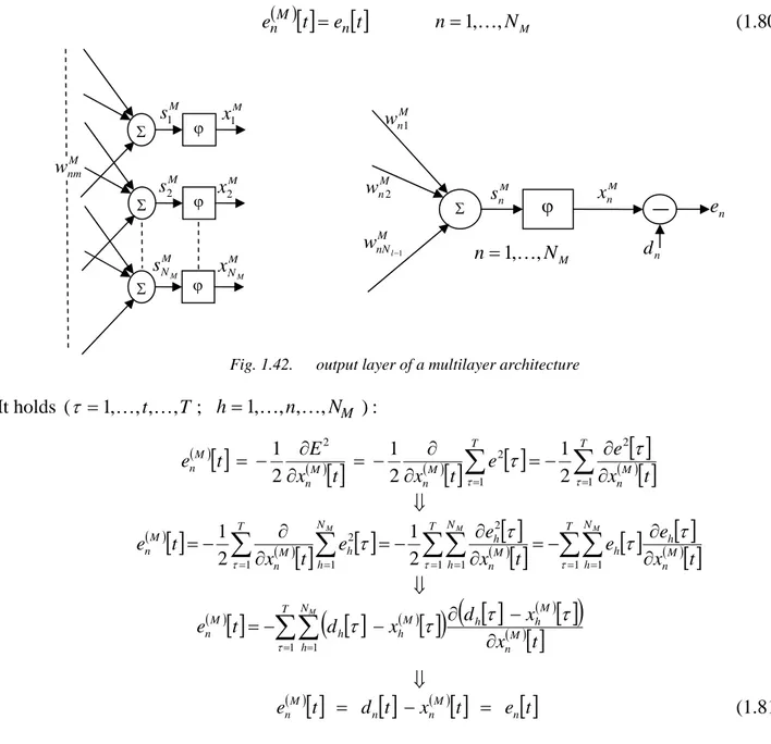
= − = M M n n N n x d E 1 2 2 1 (1.15)

The error for the generic output neuron x_n( )M is simply:

( ) ( )M n n M n =d −x δ (1.16)

As regards the hidden units, we must propagate the error back, starting from the output neurons (hence the name of the algorithm). Again, using the chain rule, we can expand the error of a hidden unit in terms of the errors relative to the neurons of the layer that follows. The output error can be

Neural network approach to problems of static/dynamic classification

UNIVERSITY OF ROME

“TOR VERGATA”

Faculty of Engineering

Ph. D. Thesis on Engineering of Sensory and Learning Systems:

“N

eural network approach to Problems of

Static/Dynamic Classification”

Supervisor

Assistant

Supervisor

Prof. Mario Salerno

Ing. Giovanni Costantini

Ph. D. Student

Ing. Massimo Carota

CONTENTS

Abbreviations and symbols

M

l

N

n

T

t

[ ]

[ ]

(

)

(

)

w

v

( )

( )

( )

[ ]

[ ]

[ ]

(

)

t

N + 1

( )

( )

P

REFACE

I

NTRODUCTION

C

HAPTER

1

NEURAL

NETWORKS

1.1 The Brain, the nervous system and their model

1.1.1 The Biological Neuron

1.1.2 Synaptic Learning

1.2 Artificial Neuron Networks Models

1.2.1 A Simple Artificial Neuron

N

(

)

(

)

∑

x

w

x

x

x

x

w

w

w

w

∑

x

( )

∑

w

x

( )

_w

_v

_{[ ]}

_{[ ]}

_{( )}

_{( )}

_∑

_∑

_∑