Application and comparison of two analytical tools of decision support for the management of resources in a river basin in Tunisia

(1)

TUSCIA UNIVERSITY OF VITERBO

-ITALY-

DEPARTMENT OF TECHNOLOGY, ENGINEERING AND

ENVIRONMENT AND FOREST SCIENCES (DAF)

PHD IN SCIENCES AND TECHNOLOGIES FOR THE FOREST

AND ENVIRONMENTAL MANAGEMENT- XXIII CYCLE

SCIENTIFIC SECTOR- DISCIPLINARY AGR/10 RURAL CONSTRUCTION

AND FORESTRY LAND

PhD Thesis

Presented by

Moez Sakka

APPLICATION AND COMPARISON OF TWO ANALYTICAL

TOOLS OF DECISION SUPPORT FOR THE MANAGEMENT OF

RESOURCES IN A RIVER BASIN IN TUNISIA.

.

Coordinator

Supervisor

Prof. Gianluca Piovesan

Dr. Antonio Lo Porto

(2)

UNIVERSITÀ DEGLI STUDI DELLA TUSCIA

-VITERBO-

DIPARTIMENTO DI TECNOLOGIE, INGENERIA E SCIENZE

DELL‘AMBIENTE E DELLE FORESTE

CORSO DI DOTTORATO DI RICERCA IN SCIENZE E

TECNOLOGIE PER LA GESTIONE FORESTALE ED

AMBIENTALE-XXIII CICLO SETTORE

SCIENTIFICO-DISCIPLINARE AGR/10 COSTRUZIONE RURALI E

TERRITORIO AGROFORESTALE

Tesi di Dottorato di Ricerca

Dottorando

Moez Sakka

APPLICAZIONE E CONFRONTO DI DUE STRUMENTI DI

ANALISI PER IL SUPPORTO ALLA DECISIONE PER LA

VALUTAZIONE DELLA DEGRADAZIONE DEL TERRITORIO

IN UN BACINO IDROGRAFICO IN TUNISIA.

Cordinatore

Tutor

Prof. Gianluca Piovesan

Dr. Antonio Lo Porto

(3)

i

ACKNOWLEDGEMENTS

This thesis would not have come to fruition without the support and encouragement of different individuals and organizations. First and foremost, I would like to extend my deepest gratitude to my advisor, Antonio Lo Porto. His interest to the study, serious follow-up, proper guidance, constant encouragement, and insightful and timely comments has been invaluable in shaping and enriching the dissertation. His valuable assistances in other matters are also gratefully acknowledged. I have learned many other qualities from him.

I would like to express my most sincere gratitude to Dr. Anna Maria De Girolamo for her precious help.

Thanks also to the Tuscia University of Viterbo (Italy) for the opportunity provided to me to attain this academic objective. Specially, I would also like to express my sincere thanks to Prof. Gianluca Piovesan.

Thanks also to the examiners who provided valuable feedback, Prof.ssa Manuela Romagnoli, Dott.Alessio Papini and Dott. Giacomo Certini.

I would also like to express my sincere thanks to Mr Habib Ghannem, Mohamed Kefi from CRDA (Commissariats Régionaux au Développement Agricole) of kairouan and Salah Mantouj from CRDA of Seliana for the Merguellil database that they provided to me.

I wish to express my sincere gratefulness to the IRD (Institut de Recherche et de Development) researchers in particular Dr. Christophe Cudennec.

I would like to express my most sincere gratitude to my director Giorgio Galli, Ing Pretner, Ing Parravicini and all the SGI Studi Galli ingegneria staff for their significant help and encouragement.

My heartfelt gratitude goes to my lovely wife, Khaoula, for her constant encouragement, patience and strength during 3 years. Special thanks to my little daughter, Elaa, whose birth has filled our home with immense joy.

(4)

ii

DEDICATION

This thesis is dedicated to:

The Memory of my dear father, May God bless you

My mother who has elevate me. You have been source of motivation to me throughout my life , you have been with me every time in my life, Thank you for all the love, guidance, and support that you have always given me, and helping me to succeed. Thank you for everything.

My father-in-law Youssef, I never stopped respecting you and I will always follow your advices, Thanks for your love and encouragement, I give my deepest expression of love and appreciation for the support to you and your wife Emna specially for her never ending moral

support and prayer

My lovelywife for her love and constant encouragement, patience and strength during our matrimony. you have been a great source of encouragement and motivation throughout the

years

My little daughter, Elaa, whose birth has filled our home with immense joy.

My family: Ali, Walid, Dorra, Olfa, Chadlia,Yasmine, Sarra, Rayen,Meriam, little Youssef,Mohamed Ali and, Radhia, Thank you for your continual love, support, and patience

My wife family Mbia, Tarek, Hatem, Iikram, Ines and Olfa for their encouragement and wishes of successful accomplishment.

My friends Aziz, Sami, Radhwen Houssemdine, Farachichou, Raouf. Ons, Makram, Mohsen, Sabrine, Raed , Abdelkader, Hamid, Giorgia, Soraya, Thanks for always being here for me.

My most sincere appreciation goes to all my friends, at IAM Bari and INAT, You have all made it a unforgettable time of my life.

Yours sincerely

(5)

iii

ABSTRACT

The objective of this study was to adapt and evaluate the applicability of a physically-based spatially distributed hydrological model SWAT (Soil Water Assessment Tool) and IWRM integrated water resources management lumped model WEAP (Water Evaluation And Planning) for simulating the main hydrologic processes in arid environments. The models were applied to the 1200-km2 watershed of wadi Merguellil in central Tunisia to investigate the hydrological response of the basin. The sensitivity analysis of hydrology, soil and vegetation parameters of SWAT and WEAP helped to identify influential parameters and this could serve as a guide in calibrating the models. The main adjustment for adapting WEAP and SWAT model to this dry Mediterranean watershed was the inclusion of water soil conservation works WSCWs, which capture and use surface runoff for crop production and aquifers recharge in upstream basins. The models were run and the simulated runoff values were compared with the measured stream-flow values. In the calibration period the Nash efficiency coefficient for the SWAT and WEAP models were respectively 0,64 and 0,41 for the runoff. The value of Nash coefficient indicates that the result of SWAT model is acceptable contrasting the WEAP model. SWAT simulation was better than WEAP in most case and could be used with reasonable confidence for runoff quantification in the Merguellil watershed. For the SWAT model, The results of the water balance simulation at monthly and annual time scales was generally good and the observed stream-flow in Zebess, Skhira, Haffouz and El Houareb flow-gages could be reproduced satisfactorily. An estimation of the suspended sediments and nutrients loads in the watershed was performed without calibration because of missing data. Several hypothetical scenarios of land use and climate change were generated by the SWAT and WEAP models in order to determine the impact of the variation of land management and climate change on water demand and supply on downstream water users.

(6)

iv

RIASSUNTO

L’obiettivo del presente studio è quello di adattare e valutare il campo di applicazione del modello idrogeologico bidimensionale physically-based SWAT (Soil Water Assessment Tool), Strumento di valutazione di acqua e suolo, e del modello WEAP (Water Evaluation And Planning), Valutazione e pianificatione delle risorse idriche, per l’analisi integrata della gestione delle acque, IWRM (Integrated Water Resources Management), al fine di simulare i principali processi idrologici in ambienti aridi.

Nella fattispecie, i modelli sono stati applicati al bacino dello Wadi Merguellil, che si trova nella parte centrale della Tunisia e si estende su di una superficie pari a 1200 Km2.

L’analisi di sensibilità dei parametri idrogeologici, di suolo e vegetazione dei modelli SWAT e WEAP, ha permesso l’identificazione dei parametri determinanti che possono essere utilizzati come linea guida nella calibrazione dei modelli stessi.

Il principale aggiustamento per l’adattamento dei modelli, WEAP e SWAT, al bacino mediterraneo arido, oggetto di studio, è stata l’introduzione della componente WSCWs, Water soil conservation works, contenente le misure per la conservazione di suolo ed acqua; tale componente permette di catturare ed usare l’acqua di ruscellamento, per la produzione di raccolti e per la ricarica dei bacini a monte del bacino stesso.

I modelli sono stati messi a punto ed i valori di deflussi simulati sono stati paragonati a quelli delle portate di deflusso stream-flow misurate a valle del bacino.

Nel periodo di calibrazione il coefficiente di efficienza di Nash, per i modelli SWAT e WEAP ha assunto rispettivamente valori di 0.64 e 0.41, per quanto riguarda i valori di deflussi. Secondo tali valori di Ens il modello SWAT risulta accettabile in contrasto con i risultati del modello WEAP. Pertanto. la simulazione ottenuta tramite il modello SWAT risulta migliore di quella ottenuta con il modello WEAP nella maggioranza dei casi. Il modello SWAT può essere dunque utilizzato con un livello di confidenza ragionevole per quanto riguarda la quantificazione del ruscellamento nel bacino di Merguellil.

I risultati della simulazione del bilancio idrico su scala mensile ed annuale, è stata generalmente buona e le portate di deflusso osservate alle stazioni di misura di Zebess, Skhira, Haffouz e El Houareb hanno potuto essere riprodotte in maniera soddisfacente.

Una stima quantitativa dell’erosione e del carico dei nutrienti nel bacino è stata condotta senza possibilità di calibrare i risultati a causa della scarsità di dati.

(7)

v

Diversi scenari ipotetici di uso del suolo e cambiamento climatico sono stati generati attraverso i modelli SWAT e WEAP, così da determinare l’impatto della variazione di tali fattori, uso del suolo e cambiamento climatico, sull’ approvvigionamento idrico degli utenti a valle del bacino stesso.

(8)

vi

LIST OF FIGURES

Figure 1 Elements of the hydrologic cycle (Chow et al., 1988) ...6

Figure 2 Schematic representation of the land phase of the water Cycle (Starosolszky, 1987) .9 Figure 3 Classification of hydrological models. Based on Becker and Serban (1990) ... 20

Figure 4: Overview of nitrogen flow models (Payreaudeau, 2002) ... 29

Figure 5 Representation of the SWAT model process ... 36

Figure 6 Components of a reservoir with flood water detention features ... 39

Figure 7 Characterization of (a) pre- and (b) post-watershed development that highlights the implications of water resource infrastructure on the hydrologic cycle ... 41

Figure 8 Physical hydrology component of WEAP21 with two different hydrologic realities. (Yates and al, 2005) ... 48

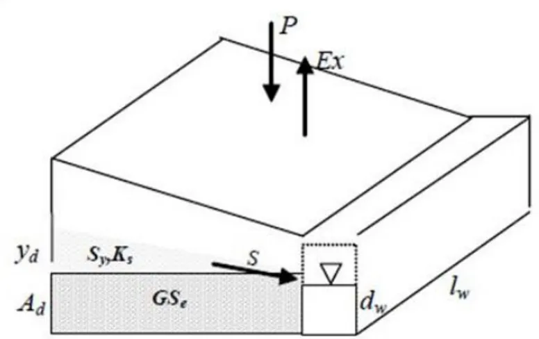
Figure 9: Schematic of the stylized groundwater system, and its associated variables (Yates and al, 2005) ... 49

Figure 10 WEAP21’s GUI for specifying in-stream flow requirements. The left panel shows the supply priority of in-stream flow, while the right panel is the actual in-stream flow requirement in m3/s that abruptly changes over time as a result of regulatory requirement .... 52

Figure 11 The different reservoir storage volumes used to describe reservoir operating ... 53

Figure 12 Location of the study area ... 57

Figure 13 Soil map of the Merguellil catchment ... 59

Figure 14 Land use map of the Merguellil catchment ... 60

Figure 15 Mean monthly precipitations in the Merguellil catchment based on measured data in all rain-gages from 1990 to 2005 (Abouabdillah, 2010) ... 61

Figure 16 Mean monthly temperatures in the Merguellil catchment based on measured data in Sbiba, Makther and kairouan stations from 1972 to1982 (Abouabdillah, 2010) ... 62

Figure 17 El Houareb Dam on May 2007 (left) and on May 2008 (right) ... 63

Figure 18 Water level of the El Haouareb dam (because of siltation, the lowest levels, recorded in 1994, 1997–2005 and 2008, correspond to a complete drying up of the dam). .... 64

Figure 19 Water infrastructure in the Merguellil basin. ... 65

Figure 20 Contour ridges in the Merguellil catchment (Dridi, 2000) ... 67

Figure 21 Assessment of average flows of the upstream zone of Merguellil basin ... 70

(15)

xiii

Figure 23 Population density per delegation in 1994(Le Goulven and al, 2009) . ... 73

Figure 24 Digital Elevation Model of the Merguellil watershed ... 75

Figure 25 Comparison of stream from SWAT and IDRISI ... 76

Figure 26: Hydrographic network extracted at surface drainage threshold of 2100 ha ... 77

Figure 27: Hydrographic network extracted at surface drainage threshold of 1000 ha. ... 77

Figure 28 Subbasins delineation in the Merguellil catchment ... 78

Figure 29 Land use map of Merguellil catchment extracted from GIS project Mergusie... 81

Figure 30 Textural triangle (Rawls, 1983) ... 84

Figure 31 integration of weather data in SWAT model interface ... 86

Figure 32 Localization of the rainfall stations retained for the study area. ... 89

Figure 33 WEAP Software diagram ... 92

Figure 34 Location of the study area, limits of the upper and lower sub-basins and of the different aquifers ... 93

Figure 35 Construction of the model: creation of the area ... 93

Figure 36 : WEAP input: Average monthly Precipitation in the Merguellil watershed ... 94

Figure 37 Monthly variation for water demand in the Merguellil Watershed ... 97

Figure 38 Monthly Natural recharge Haffouz aquifer ... 98

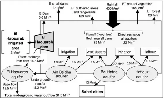
Figure 39 Water balance of the Merguellil watershed (Le Gouleven and al, 2009). ... 100

Figure 40 Water balance in the downstream of the Merguellil watershed ... 101

Figure 41 WEAP model for Merguellil catchment ... 102

Figure 42 Sensitivity of the SWAT model to the soil-vegetation parameters ... 106

Figure 43 Sensitivity of the SWAT model to the groundwater parameters ... 107

Figure 44 Sensitivity of the SWAT model to the hydrographic network parameters ... 108

Figure 45 Sensitivity of the SWAT model to the erosion parameters... 109

Figure 46 Sensitivity of the SWAT model to the Phosphorus and Nitrate parameters ... 110

Figure 47 Flow variation for different threshold of discretization of Merguellil Watershed . 112 Figure 48 Variation of the concentration of suspended solids for different subdivision thresholds of Merguellil watershed ... 112

Figure 49 Variation of the concentration of nutrients for different thresholds subdivision of Merguellil watershed. ... 113

Figure 50 Flow gage (red dots) used for calibration and validation of the hydrological model SWAT ... 118

(16)

xiv

Figure 52: contour ridges map of Merguellil catchment on 2003 (CRDA KAIROUAN-IRD)

... 122

Figure 53 Location of small dams within the Merguellil watershed ... 124

Figure 54: Evolution of contour ridges map of Merguellil catchment (Dridi, 2000) ... 126

Figure 55 overlaid aquifers maps and subbasin map generated by swat ... 130

Figure 56 overlaid Water harvesting maps (MERGUSIE PROJECT-CRDA) and subbasin discretisation map generated by SWAT model ... 131

Figure 57: Observed and simulated yearly flow for the Skhira (left) and Zebbess (right) gauging station ... 133

Figure 58: observed and simulated yearly flow for the Haffouz gauging station and the Merguellil watershed ... 133

Figure 59 The water balance of the watershed Merguellil for an annual simulation ... 134

Figure 60 Variation of monthly measured and simulated stream flows by SWAT at the gauging station Skhira before calibration. ... 135

Figure 61 Variation of monthly measured and simulated stream flows by SWAT at the gauging station Zebbess before calibration ... 136

Figure 62 Variation of monthly measured and simulated stream flows by SWAT at the gauging station Haffouz before calibration ... 136

Figure 63 Variation of monthly measured and simulated stream flows by SWAT at the Merguellil watershed outlet before calibration ... 137

Figure 64: Observed and predicted monthly streamflow at Skhira after calibration ... 138

Figure 65: Observed and predicted monthly streamflow at Zebbess statio after ... 138

Figure 66: Observed and predicted monthly streamflow at Haffouz station after calibration ... 138

Figure 67: Observed and predicted monthly streamflow at watershed outlet after calibration ... 138

Figure 68 The water balance of the watershed Merguellil for an monthly simulation (September) ... 139

Figure 69 The water balance of the watershed Merguellil for an monthly simulation (March) ... 139

Figure 70 Variation of daily measured and simulated stream flows by SWAT at the gauging station Skhira before calibration ... 140

Figure 71 Variation of daily measured and simulated stream flows by SWAT at the gauging station Zebbess before calibration ... 141

(17)

xv

Figure 72 Variation of daily measured and simulated stream flows by SWAT at the gauging

station Haffouz before calibration ... 142

Figure 73 Variation of daily simulated stream flows by SWAT at the Outlet Merguellil watershed ... 143

Figure 74: Observed and predicted daily streamflow at Skhira gauging station after calibration ... 143

Figure 75: Observed and predicted daily streamflow at Zebbess gauging station after calibration ... 143

Figure 76: Observed and predicted daily streamflow at Haffouz gauging station after calibration ... 144

Figure 77: predicted monthly streamflow at daily watershed outlet after calibration ... 144

Figure 78 Sediments Concentration and Sediments Average yearly loads simulated at the watershed outlet. 1992-2002 ... 144

Figure 79 Sediments Concentration and Sediments Average yearly loads, simulated at the Skhira subbbasin 1992-2002 ... 144

Figure 80 Sediments Concentration and Sediments Average yearly loads simulated at the Haffouz subbbasin 1992-2002 ... 145

Figure 81 Sediments Concentration and Sediments average monthly load simulated at Skhira for the period (1992-2002) ... 147

Figure 82 Sediments Concentration and Sediments average monthly load, simulated at the Zebbess subbbasin (1992-2002) ... 147

Figure 83 Sediments Concentration and Sediments average monthly load, simulated at the Haffouz subbasin for the (1992-2002) ... 147

Figure 84 Sediments Concentration and Sediments average monthly load, simulated at the outlet for the period (1992-2002) ... 147

Figure 85 Sediments average daily load simulated at the Haffouz subbbasin for the period (1992-2002) ... 148

Figure 86 Sediments Concentration simulated at the outlet for the period (1992-2002) ... 148

Figure 87 Annual variation of the of nitrate load at Merguellil watershed outlet ... 149

Figure 88 Annual variation of the of nitrate load at Merguellil watershed outlet ... 149

Figure 89 Daily variation of the of NO2 load at the Merguellil watershed outlet for the period (1992-2002) ... 150

Figure 90 Daily variation of the of NO3 load at the Merguellil watershed outlet for the period (1992-2002) ... 150

(18)

xvi

Figure 91 Daily variation of the of NH3 load at the Merguellil watershed outlet for the

period (1992-2002) ... 150

Figure 92 Daily variation of the mineral phosphorus loaded at Merguellil watershed. ... 151

Figure 93 : Spatial distribution of nitrate losses in the watershed Merguellil ... 152

Figure 94 : Spatial distribution of nitrate losses in the watershed Merguellil ... 152

Figure 95 Impact of irrigation scenario (April and May) on monthly water volume in the outlet - Scenario 1: provide 60 mm of irrigation from rivers - Scenario 2 provide 30 mm irrigation from river and 30 mm from aquifer. ... 153

Figure 96 Variation of nitrate concentration in the river for the 2 scenarios ... 154

Figure 97 Impact of the intensification of water harvesting systems "ponds" on the average monthly stream flow in the Skhira subbasin ... 155

Figure 98 Impact of the intensification of water harvesting systems "ponds" on the average monthly stream flow in the Zebbess subbasin ... 155

Figure 99 impact of the intensification of water harvesting systems "ponds" on the average monthly stream flow in the Haffouz subbasin. ... 155

Figure 100 : Sensitivity of the model to crop coefficient ... 157

Figure 101 Sensitivity of the model to effective precipitation ... 157

Figure 102 Sensitivity of the model to runoff/infiltration ratio ... 157

Figure 103 Sensitivity of the model to hydraulic conductivity ... 157

Figure 104 Comparison of simulated and observed yearly flow (1992-2002). ... 158

Figure 105 Comparison of simulated and observed monthly flow (1992-2002 ). ... 159

Figure 106 Water demand for agricultural and domestic sites in the Merguellil watershed .. 159

Figure 107 Annual water demand for agricultural and urban sites. ... 160

Figure 108 Annual Groundwater Inflows and Outflows in the Merguellil watershed ... 160

Figure 109 Ainbidha aquifer inflow- out flow in period 1992-2002 ... 161

Figure 110 Climate change scenario in the Merguellil watershed 2002-2020 ... 162

Figure 111 Impact of climate change on Haffouz aquifer inflow-outflow ... 163

Figure 112 Average monthly Demand site coverage 1992-2020 ... 164

Figure 113 Monthly average water demand for all the site (agriculture and urban) 1992-2020 ... 165

(19)

xvii

LIST OF TABLES

Table 1 Relationship between time step of modeling and area of catchment (Adapted from

Starosolszky (1987) ... 18

Table 2: assessment of SWAT and WEAP models ... 31

Table 3 Assessment of green water consumption according to rainfall. ... 71

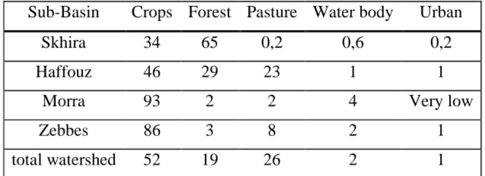
Table 4 : Land use in subbasin (in %) in the Merguelli watershed (Dridi, 2000) ... 81

Table 5: Soil Characteristics of the four soil types considered in the watershed Merguellil. The texture is expressed as% of clay, silt and sand ... 83

Table 6 Input Soil Unit data in the Merguellil watershed ... 86

Table 7 Altitude and location of temperature gage selected for the study ... 87

Table 8: mean monthly temperatures (° C) (1979 - 2002) ... 87

Table 9: Mean maximum monthly temperature (°C) average 1979 - 2002 ... 87

Table 10: Mean minimal monthly temperature (°C) 1979- 2002 ... 88

Table 11 Geographical locations of rainfall gages in the watershed Merguellil (DGRE) ... 88

Table 12 Monthly Kc input for the study area ... 94

Table 13 Water demand site ... 96

Table 14 Groundwater data required for WEAP model ... 98

Table 15 Transmission Link between water supply site and demand site... 100

Table 16 Parameters selected for the sensitivity study ... 105

Table 17 Erosion parameters selected for the sensitivity study ... 108

Table 18 Phosphorus and Nitrate parameters selected for the sensitivity study ... 110

Table 19 Number of sub basins obtained for different threshold surface drainage. ... 111

Table 20 : Characteristics of flow gages in Merguelli catchment (Kingumbi, 1999) ... 117

Table 21 Simulation period based on WSCW distribution ... 123

Table 22 : Distribution of the small dam’s period of simulation sub-basin ... 126

Table 23 Small Dams on the catchment Merguellil ... 127

Table 24: Groundwater parameters after adjustment: coefficients for recession (alpha), evaporation (revap) and recharge to the deep aquifer (rchdp), response delay and Threshold to allow base flow to the river (gwqmin in mm) ... 131

(20)

xviii

Table 26 : statistics coefficients calculated for the monthly calibration of the SWAT model

... 139

Table 27 : statistics coefficients calculated for the daily calibration of the SWAT model ... 140

Table 28 Masses and concentrations of sediment load in the watershed outlet and Skhira subbasin ... 145

Table 29: Comparison of specific erosion result in Skhira subbasin ... 146

Table 30 Comparison of specific erosion result in Haffouz subbasin ... 147

Table 31: Concentration of NO2, NO3 and NH at the Merguellil watershed ... 151

Table 32 Impact of the intensification of water harvesting systems "ponds" on streamflow in the Merguellil watershed management ... 156

Table 33 Variations of the Least Squares Objective function and of the mean annual simulated flow due to changes in the parameter values. ... 156

(21)

xix

LIST OF APPENDICES

APPENDIX 1 : SOIL PROFILES (DIRECTION DES SOLS 1963-1982) ... 187 APPENDIX 2 LANDUSE/SOIL DISTRIBUTION CLASS IN THE MERGUELLIL CATCHMENT WITH SWAT MODEL ... 191

(22)

xx

ABBREVIATIONS

CES Conservation Des Eaux Et Du Sol.

CGCM Generation Of The Canadian Global Coupled Model

CO2 Carbon Dioxide

DEM Digital Elevation Model DGF Direction Générale Des Forêts

DGRE Direction Générale Des Ressources En Eaux

ET Evapotranspiration

GIS Geographic Information System

GLUE Generalised Likelihood Uncertainty Estimation GTZ Technische Zusammenarbeit Gmbh

HOF Hortonian Overland Flow

HU Heat Unit

HRUS Hydrologic Response Units

IPCC Intergovernmental Panel On Climate Change NERC Natural Environment Research Council SCS Soil Conservation Service

SWAT Soil And Water Assessment Tool USA United State Of America

USDA United States Department Of Agriculture USEPA United State Environmental Protection Agency USGS United States Geological Survey

WSCW Water And Soil Conservation Works

PHU Plant Heat Units

PET Potential EvapoTranspiration

MUSLE Modified Universal Soil Loss Equation ESRI Environmental Systems Research Institute RUE Radiation-Use Efficiency

SCS-CN Soil Conservation Service-Curve Number IGNF Institut Géographique National Français IRD Institut De Recherche et de Développement

TP Total Porosity

FC Field Capacity

WP Wilting Point

AWC Available Water Capacity

INM Natural Resource Conservation Service IRCS Institut National De Météorologie UTM Universal Transverse Mercator

AVFA Agence De Vulgarisation Et Formation Agricole Ens Nash-Sutcliffe Model Efficiency

R2 Coefficient Of Determination WEAP Water evaluationand planning

(23)

1

1 INTRODUCTION

1.1 PROBLEM STATEMENT

Despite the critical importance of water scarcity, the hydrology in semi-arid regions has not received as much attention as other climatic regions and historically the hydrological data have been severely limited and can in some respects be categorized as ungauged basins. The limitation of data is due a small population density and hydrological observation networks are difficult and costly to build and maintain in such regions. Furthermore, hydrological extremes are more common than in humid climates among others due to the following: 1) precipitation is low on an annual basis but it falls as high-intensity storms of often limited spatial extent, 2) high potential evaporation, and 3) low runoff volume on an annual basis and runoff occurs as short intermittent flash floods. In order to develop a successful recharge estimation approach for a region, the effects of all the complex mechanisms must be taken into account.

Hydrological models are valuable, if not essential tools for this purpose. They have become a basic tool in hydrology. Their development, which was closely linked to increasing power of computer processing, started in the 1960s. They are now indispensable tools for planning, design and management of hydrologically related infrastructure. They can also improve system understanding which is required for decision making and policy analysis. The advantage of hydrological models is that all the terms of the water balance can be estimated over an unlimited time frame. Various model approaches have been proposed for this purpose ranging from simpler lumped and conceptual catchments models to complex distributed and physically based models. Compared with lumped models distributed hydrological models can account for spatial heterogeneities and provide detailed description of the hydrological processes in a catchment. However the main disadvantage of these models is the high demands of spatial input data.

The water management literature is rich with integrated water resources management IWRM models that have tended to focus either on understanding how water flows through a watershed in response to hydrologic events or on allocating the water that becomes available in response to those events. For example, the US Department of Agriculture’s Soil Water Assessment Tool (SWAT, (Arnold and Allen, 1993), includes sophisticated physical hydrologic watershed modules that describe, among others, rainfall-runoff processes, irrigated agriculture processes, and point and non-point water watershed dynamics, but a relatively

(24)

2

simple reservoir operations module (Srinivasan et al., 1998; Ritschard et al., 1999; Fontaine et al., 2002).

Nevertheless, the number of hydrological models now available has increased to such an extent that it has become a relatively hard task to choose one from amongst them all when a simulation is to be done. Selection of an appropriate model for a particular need is made easier thanks to several model classifications that have emerged in the past (Schulze, 1998). Hydrological models are usually distinguished on the basis of their:

- Function: prescriptive models are used to make predictions of catchment behavior and are used in engineering and regulation studies. Descriptive models

are more specifically concerned with testing of conceptual theory and mainly applied in scientific research.

- Structure: three groups of models exist depending on their structure. Deterministic models are physically-based and describe cause and effect relationships with mathematical equations. Stochastic models use statistical properties of existing records and probability laws to solve hydrological problems. Conceptual models average inputs/outputs of an area to get rid of time and space heterogeneities that constitute a hydrological system.

- Level of spatial disaggregation: lumped models represent processes in a spatially averaged way whereas distributed models represent them in a spatially disaggregated way.

Criteria for the selection of a model are mainly linked to the nature of the problem to be evaluated and to the resources available (data, computing facilities). The naïve perception that model complexity is positively correlated with confidence in the results has faded in the recent years and the whole concept itself of physically-based hydrological modeling has been brought into question (Grayson et al., 1992): it must be kept in mind that equations underlying these models describe processes occurring in structurally stationary ‘model’ catchments which are spatially homogenous at the model grid-scale (Beven, 1989). Consequently, accuracy of the model depends on the degree of heterogeneity that is lumped in it, and improving descriptions without introducing parameter identifiability problems, this is a question that is still not resolved (Beven, 2000).

(25)

3

1.2 RESEARCH OBJECTIVES

Modeling can play a key role in the development of sustainable management of water resources at river basin scale. Modeling can help in evaluating current water resources, identify pollution sources (source apportionment), evaluate alternative management policies, and elaborate sustainable water allocation among various stakeholders. Various studies investigated the role of models in the implementation of the water related policies such as the EU Water Framework Directive (Wasson and Tusseau, 2003; Dørge and Windolf, 2003). Fewer efforts have been dedicated to the use of models in Northern African countries in helping the evaluation of the implementations of policies, especially those dealing with agriculture (Bouraoui and al, 2005).

The objective of this study is to investigate the spatial and temporal variation of water resources in

the semi-arid basin through hydrological modeling, the Water Evaluation And Planning (WEAP) model, a lumped model, and Soil Water Assessment Tool (SWAT) were used to simulate the hydrology of the Merguellil catchment. The aims of the study were:

- to evaluate the rainfall-runoff component of both models and to test their ability to compute natural flow data.

- to assess the impact of development on water resources by simulating water uses in the catchment.

- to provide information about two models ability to be used as a water management analysis and planning tool in the Merguellil catchment.

- to adapt the models to this dry Mediterranean environment by the inclusion of water harvesting systems (contour ridges and small dam), which capture and use surface runoff in upstream subbasins.

- To analyze the flow regime alterations and water demand under scenario of land use and climate change

- To compare the result of SWAT and WEAP models

1.3 OUTLINES OF THE THESIS

After describing the context of the study and introducing the objectives of the thesis in the Chapter 1, the whole purpose of the chapter 2 is to provide a wider literature review for the research by highlighting some of components of the hydrological cycle in the watershed. The

(26)

4

importance of scientific researches in the areas of hydrology, in the semi arid context is presented. In line with the objectives of this study, an overall presentation on the types of hydrological models and their applications in water resources management is made.

Chapter 3: This chapter is dedicated to the description of physically-based distributed hydrological model (SWAT) and the lumped model WEAP used in the study. The different hydrological processes, input requirements and outputs of the model are described. Moreover, some examples of the model application from around the world are included.

Chapter 4: The status of water resources development in Tunisia in general and Merguellil, in particular, is briefly presented in the chapter. This chapter describes the environment of the study area. It begins with the presentation of the environment of the study area in terms of its geographic and climatic characteristics. This is followed by sections on soil and land cover types and geology of Merguellil basin. An overview of the climate and hydrological systems of the study area is also included. Available data base such as the DEM, soils, land uses, and Water and Soil Conservation Works (WSCW) are presented. Analysis of the climatic data in the catchment involved checks on data quality and consistency, gap filling, and temporal and spatial characterizations.

Chapter 5: This chapter deals with the description the data required by two models. First part is dedicated to the SWAT setting parameter. The inputs required by the models including soil and land use data, (like soil hydraulic properties, digital elevation model etc) we describe the adaptation of the input data and how we model the different WSCW presented in the catchment. In the second part of this chapter, we describe the WEAP model with the different equations used and the different procedure of the simulation. The existing data related to quantification of water demand and water supply on the watershed, is explained. The required input data for the WEAP model are prepared in this chapter.

Chapter 6: Application of the two, physically-based distributed hydrological and lumped models to Merguellil catchments is presented in this chapter. As the model comprises several parameters, identification of few influential parameters is important to facilitate the calibration task. To this end sensitivity analysis of the models parameters was made and the results are presented.

An overview of methods used for calibration and validation of hydrological models is included in the first part. This is followed by the procedures used in calibrating and validating the model on the selected catchment. Comparing the measured and simulated flow in different

(27)

5

flow gauges are reported in this chapter. The SWAT model was run at time step from yearly to monthly to daily time scale on selected catchment while The WAEP model was run at time step from yearly to monthly time scale. Determination of the water balance and suspended sediment and nutrient loads in Merguellil watershed is one of the drivers of this chapter. Finally, some scenarios of land use for the SWAT model are examined. Also scenario of climate change until 2020 year is generated with WEAP model to predict hydrologic component and water demand and supply. The modeling results and their implications are finally discussed. Finally, overall conclusion and perspectives are presented.

(28)

6

2 CHAPTER 2: LITERATURE REVIEW

2.1 COMPONENTS OF THE HYDROLOGICAL CYCLE

The central focus of any hydro-meteorological study is the hydrological cycle shown in figure 1. The hydrological cycle has no beginning or end and its many processes occur continuously (Chow et al., 1988). In describing the cycle, the water evaporates from ocean and land surface to become part of atmosphere; water vapor is transported and lifted in the atmosphere until it condenses and precipitates on the land or the oceans. Precipitated water may be intercepted by vegetation, becomes overland flow over the ground surface, infiltrate into the ground, flow through the soil as subsurface flow and discharges into streams as surface runoff. The infiltrated water may percolate deeper to recharge groundwater, later emerging as spring and seeping into streams to form surface runoff and finally flowing into the sea or evaporating into the atmosphere as the hydrological cycle continues.

Figure 1 Elements of the hydrologic cycle (Chow et al., 1988)

It is noted that though the concept of the cycle seems simple, the phenomena are enormously complex and intricate. It is not just one large cycle but it is rather composed of many interrelated cycles of continental, regional and local extent. The major achievement and objectives of the rainfall runoff modeling is thus to study a part of the hydrological cycle,

(29)

7

namely the land phase of the hydrological cycle on a catchment scale. Then the problem becomes to express the runoff from the catchment as a function of the rainfall and other catchment characteristics.

2.1.1 PRECIPITATION

Precipitation is the input to the system of catchment, which may have different forms, rainfall, storms, dew or any form of water landing from atmosphere. The amount of precipitation can be defined as an accumulated total volume for any selected period. Precipitation as a function of time and space is highly variable. Systematic averaging methods such as Thiessen polygon, isohyte and reciprocal distance methods have been developed to account for variations in space to obtain a representation of areal precipitation values from point observation. Singh and Chowdhury, (1986) after comparing the various methods for calculating areal averages, concluded that all methods give comparable results, especially when the time period is long. For short time step records, the conversion of a point observation to an areal rainfall has a large influence.

2.1.2 EVAPORATION AND TRANSPIRATION

Catchment evaporation demand is generally defined as that evaporation which would occur if there were no deficiencies in the availability of moisture for evapotranspiration by that area's particular plant regime. The two main factors influencing evaporation from an open water surface are the supply of energy to provide latent heat of vaporization and the ability to transport the vapor away from the evaporative surface: solar radiation and wind. Evapotranspiration from land surface comprises evaporation directly from the soil and vegetation surface and transpiration through plant leaves, in which water is abstracted from the sub soil. The third factor is the supply of moisture at evaporative surface, which brought about the definition of potential and actual evaporation. Evaporation involves a highly complex set of processes, which themselves are influenced by factors dependent on the local conditions (land use, vegetation cover, and meteorological variables). Mostly the potential evaporation is the quantity obtained either by using some simple empirical formula such as Thornthwaite, (1948), Penman formula (Penman, 1948) and a process-based model of Penman-Monteith (Monteith, 1965).

(30)

8

2.1.3 INTERCEPTION

The portion of rainfall intercepted by the vegetation and roofs before reaching the ground is referred to as interception. The water, which is intercepted by the leaves of vegetation and roofs eventually evaporates into atmosphere. The amount of interception could be significant in densely vegetated areas such as tropical rainforests. Such forests maintain a relatively consistent canopy and do not generally exhibit the seasonal range of interception encountered in areas where deciduous trees are dominant. It is commonly understood that if the density of the vegetation cover is sparse then this loss is insignificant.

2.1.4 INFILTRATION

The precipitation, which is not intercepted or evaporated from the land, will eventually infiltrate into the soil or flow as overland flow. Infiltration is one of the most difficult hydrological processes to quantify. The difficulty arises due to many physical factors affecting the rate of infiltration such as rainfall intensity, initial moisture content, soil property, etc. Some experimental and empirical formulas such as Horton (1939), Philip (1957), and others are available to compute infiltration rates during a rainfall event. Depending on the soil strata, the infiltrated water gradually percolates to the groundwater or either flows as subsurface flow supplying river or springs within the catchment.

2.1.5 STREAM FLOW

The rainfall that exceeds the interception requirement and infiltration starts to accumulate on the surface. Initially the excess water collects to fill depressions, until the surface detention requirement is satisfied. Thereafter when water begins to move down slope as a thin film and tiny streams which eventually join to form bigger and bigger channels. This part of the stream flow is termed as surface runoff. The infiltrated part of the rain may sometimes come as subsurface runoff, which combined with the surface runoff, constitutes the direct runoff. Hence the direct runoff is the result of the immediate response of a catchment to the input rainfall. The stream flow consists of the direct runoff (which lasts for hours or days depending upon the catchment size) and the base flow (that emerges from groundwater resources and also delayed subsurface runoff). The above description of the processes at catchment scale is schematically represented in Figure 2.

(31)

9

2.1.6 GROUNDWATER

Natural groundwater fluxes are typically slow; water may reside in an aquifer for as little as a few hours or for hundreds of years. Accordingly, groundwater itself is often perceived, on the average, as a relatively slow-moving reservoir in the global hydrologic cycle. At the catchment scale, however, where stream - aquifer interactions are relatively rapid and substantial, the average groundwater fluxes are relatively fast moving. They comprise: (1) the natural flow of water between watersheds, (2) the water pumped from an aquifer, (3) mountain- front recharge (seasonal infiltration of snowmelt at the base of mountain ranges), (4) event-based infiltration (infiltration from precipitation and subsequent rises in surface water levels, especially rivers), and (5) artificial recharge via anthropogenic conservation projects.

(32)

10

2.2 ROLE OF HYDROLOGY AND EROSION AND SEDIMENT TRANSFER IN

WATERSHED MANAGEMENT

Watershed management is concerned with the protection and maintenance of land and water resources. It is multidisciplinary and requires the involvement of various actors. Watershed management is an effective tool in dealing with one or more of the issues.

The roles of hydrological and sediment-related studies are explicit and direct in the problem formulation and evaluation of alternative plans. The problem formulation is a key step in the process and should indicate among others, the magnitude and frequency of the problem, priority problem areas, and causative factors. Appraisal and evaluation of impacts of alternative plans require information on the socio-economic and environmental burdens of proposed interventions. Hydrological inputs and analysis make important contribution in addressing problems of water quantity by providing basic information on water balance in space and time. Knowledge of the relative magnitudes of the various water balance components such as evapotranspiration, direct runoff, subsurface flow, soil moisture, etc. are essential in assessing adequacy of water for current and planned developments. It also helps decision makers to weigh the advantages of each proposed intervention on the hydrologic cycle against the disadvantages. Decisions made in the absence of basic hydrological inputs would entail immense socio-economic and ecological costs. Hydrology also allows assessment of land use and climate change impacts on water balance. The fact that the hydrological literature is filled with several water balance related studies, from catchment to global scale, is an indication of its importance in water management (Engida, 2010).

Soil erosion and sediment transport is a critical environmental issue because of its adverse socio-economic and environmental impacts such as loss of soil productivity, reservoir sedimentation and associated effects, and water quality impairment. Studies on soil erosion and sediment transfer contribute to effective management of the problem by providing basic information that includes sediment source areas, pathways, sediment yield, and other controlling factors. Such information, for instance, could be used to identify and prioritize critical areas for soil conservation measures.

2.3 WATER QUALITY ISSUES

Freshwater quality impairment has been a major issue of concern worldwide. The sources of water pollution can be point or diffuse sources. Point sources of pollution include municipal and industrial wastewaters for which specific points of entry to a receiving water body can be

(33)

11

identified. Diffuse sources of pollution include general land runoff from urban and agricultural areas and other sources that do not have specific discharge points. Unlike point sources, diffuse sources of pollution are difficult to manage (Novotony and Olem, 1994). Due to the extensive damages that could be caused by diffuse sources of water pollution, the need for addressing the issue as an international priority of concern was already heralded long ago (Duda, 1996). Diffuse pollution is considered to be the dominant cause of water quality impairment in many developing countries due to poor waste management and environmentally unfriendly agricultural methods.

2.4 HYDROLOGICAL CHARACTERISTICS OF SEMI-ARID AND ARID AREAS

In the past, several hydrologists attempted to classify zones of the world in to humid, semi arid and arid according to the climaticological characteristics. One of the earliest indexes (Chow, 1964) used for classification is based upon the adequacy of precipitation in relation to the needs of plants whereby the precipitation analyzed month by month is just adequate to supply all the water for maximum evaporation and transpiration in the course of a year. UNESCO (1979) attributes the arid and semiarid zones as the dry areas associated with annual potential evaporation over 1000mm and further classifies according to the amount of annual rainfall they receive to hyper-arid, arid semiarid and humid. Chow, (1964) suggests that in addition to climatic characteristics other features of the land surface may also be used to delimit arid zones, since the geomorphology, soils and vegetation have their own distinctive characteristics. The objective of these classifications is mainly to study the peculiar characteristics common to a region, which would help generalization and inference for climatological and hydrological processes prevailing in these regions.

The hydrological processes operating in rainfall runoff transformation for the semi-arid and arid areas differ from those in humid temperate. Some of the distinct properties manifested in semi-arid and arid catchments are pointed out below.

2.4.1 VARIABILITY IN TIME

The rainfall in semi-arid and arid catchments is characterized by a high variability of the small amount received in space and time (Moore, 1989). A high percentage (about 80 percent of the annual rainfall) is received within the rainy seasons during 3 to 6 months. Individual rainfall events generally occur with high intensity and short duration storms. Verma (1979) points out some of the particular features of the semiarid and arid hydrological processes as:

(34)

12

• The marked seasonal variation in semiarid climates may require segregation of data by season. A combination of hydrological factors common in one season of the year may be virtually non-existent during another season.

• A particular combination of factors may exist for only a few days in several years and may render hydrological computation based on average values grossly erroneous.

Actual evaporation from semi-arid zones is a highly transient phenomenon with extreme variation within a day because of the available water but not over a season. The transient nature of evaporation is also controlled by the rapid growth of vegetation to climax followed by rapid die-off (Moore, 1989).

2.4.2 VARIABILITY IN SPACE

In contrast to humid climate, hydrological processes in semiarid and arid regions often vary greatly over different parts of a catchment. Especially in large catchments, the contributing area could be localized at the upper part of the catchment. In such cases, computation of areal rainfall in a lumped conceptual model leads to unrealistic average distribution over the whole area. Moreover, the sparse vegetation cover and its sharp response to the first rain have an impact on the evaporation process prevailing in such regions. The rivers in such regions are generally characterized by having long periods of low flow regime.

Another distinct characteristic of such regions is that in some cases infiltration could be very small due to outcropped rocks on the slopes of valleys whereas it could be high in areas with fractured bedrock channels. There could also be the possibility of channel infiltration from the bed of the rivers supplying the groundwater in lower valleys of the river (Sami, 1992). This fact implies that especially during low flow regime the stream flow that originates from upstream will be depleted by the channel bed before it reaches the outlet. Hence this phenomenon should be accounted for in formulating models based on the water balance of a catchment

2.5 WATER AND SOIL CONSERVATION WORKS IN THE SEMI ARID ZONE

In many arid countries, runoff water-harvesting systems support the livelihood of the rural population. Little is known, however, about the effect of these systems on the water balance components of arid watersheds (Ouessar and al, 2009). Generally, water and soil conservation works (WSCW) are built in uplands to face erosion and water scarcity problems. They consist of hillslope works reducing surface runoff and increasing local infiltration, and of small dams

(35)

13

collecting headwater flow and providing supplemental water for irrigation. Intensive water uses are most often concentrated in alluvial plains that offer large and easily irrigable lands, better soils and abundant water resource through aquifer tapping.

By retaining upstream runoff, WSCW modify the spatial and social distribution of costs and benefits at the catchment scale. With the fast growth of WSCW-equipped areas, it becomes necessary to investigate hydrological impacts and manage resources at larger scales, especially where conflicts between upstream and downstream water uses increase. Although precise knowledge on the WSCW hydrological impacts is a prerequisite, it remains rare especially in large catchments (above 100 km2).

Many studies on WSCW hydrologic impact have been reported, according to land use/land-cover modifications:

• forestation, forest clearing (e.g., Leduc et al., 2001), in Niger, Siriwardena et al., 2006, in Australia)

• intensification of agricultural practices (e.g., Lorup et al., 1998, in Zimbabwe) • Climate change (e.g., Séguis et al., 2004, in the Sahel)

The few investigations on WSCW effects on catchment hydrology mainly concern changes induced by large reservoirs (e.g., Batalla et al., 2004, in Spain; Güntner et al., 2004, in northeast Brazil; Thoms and Sheldon, 2000, in Australia). Studies on impacts of hillslope works (soil bunds, contour ridges, hedges, tillage) are extremely rare in large catchments as heterogeneity and data scarcity increase with catchment size. Xiubin et al. (2003) examined the correlation between the surface area controlled by WSCW and streamflow reduction in three catchments (362 000 km2, 1121 km2 and 70 km2) of the Yellow river basin in China. They found that controlled surfaces fractions of 26.0%, 28.3% and 56.3% induced runoff decreases of 49.4%, 52.6% and 49.7% respectively. Several research works were conducted either for small catchments or at the plot level. In central Tunisia, Nasri et al. (2004b) studied the hydrological impact of contour ridges in a 18.1 km2 catchment and on a 0.11 km2 hillslope. In both cases, introduction of contour ridges resulted in a runoff decrease varying between 50% and 90% for rainfall below 60-70 mm/day. In southern Tunisia, Nasri et al. (2004a) found that a traditional system of soil banks installed in a 0.26 km2 catchment reduced the runoff to essentially zero. In Cabo Verde islands, Smolikowski et al. (2001) found that runoff occurred only for rainfall events higher than 40 mm, with an intensity above 40 mm/h, in 4 m2 and 100 m2 plots with two kinds of conservation techniques (light mulching with maize haulms and hedging with bushes and grass). In semi-arid Kenya, Wakindiki and

(36)

14

Ben-Hur (2002) evaluated the effects of indigenous WSCW on runoff from 12 plots of 12 m2, and found that these techniques reduced the runoff by half. In all these local studies, questions of up-scaling were not considered and hydrological consequences at the regional scale were not explored. At a larger scale, identifying specifically the effects on streamflow of given environmental changes is difficult because of the diversity and variability of factors controlling the runoff response to rainfall. Opposite effects may mask each other. When changes affect only a limited area of the catchment, the moderate magnitude of their impacts makes the results statistically non significant. For instance, in Australia Nandakumar and Mein (1997) found that for the level of uncertainty of their data, 65% of a 520 ha eucalyptus forest catchment would need to be cleared before flow increase could be asserted at the 90% prediction level.

2.6 RUNOFF RESPONSE IN THE SEMI ARID AREA

Factors controlling the runoff response may be grouped into two categories relating to their time variability. The first category gathers the high-frequency factors that act at the event scale. They are essentially linked to meteorological conditions. In semi-arid areas, most authors agree that rainfall intensity is the dominant control on the runoff response (Bradford et al., 1987; Canton et al., 2001; Martinez-Mena et al., 1998), whereas initial soil moisture content generally plays a secondary role (Castillo et al., 2003; Fitzjohn et al., 1998; Karnieli and Ben Asher, 1993; Peugeot et al., 2003).

These factors induce a large variability in the event rainfall-runoff relationship, making similar rainfall depths produce a large range of runoff depths. In the second category, the low-frequency factors that progressively modify the runoff response are essentially: climate change (Servat et al., 1997), land use changes (Calder et al., 1993; Fahey and Jackson, 1997), changes in the water table level, altering the flow intensity between the surface and underground (Matteo and Dragoni, 2005) and WSCW construction. When trying to identify the hydrological impact of low-frequency factors, a difficulty consists in being able to differentiate their effects from those of high-frequency factors. Hydro-meteorological data with high time/space resolution are generally used to model the relationship between high-frequency factors and runoff response. “Unexplained”, progressive changes in the catchment behavior may afterwards be attributed to low frequency factors. When data resolution is insufficient to identify the impact of high-frequency factors, the latter act as background noise

(37)

15

in the rainfall/runoff relationship. Due to this noise, long data series are needed to identify rainfall/runoff changes due to one or more low frequency factors.

2.7 LAND USE CHANGE UNDER CLIMATE CHANGE

Water management planners are facing considerable uncertainties on future demand and availability of water. Climate change and its potential hydrological effects are increasingly contributing to this uncertainty. The Second Assessment of the Intergovernmental Panel on Climate Change (IPCC, 1996) states that an increasing concentration of greenhouse gases in the atmosphere is likely to cause an increase in global average temperature of between 1 and 3.5 degrees Celsius over the forthcoming century. This will lead to a more vigorous hydrological cycle, with changes in precipitation and evapotranspiration rates regionally variable. These changes will in turn affect water availability and runoff and thus may affect the discharge regime of rivers. The potential effects on discharge extremes that determine the design of water management regulations and structures are of particular concern, since changes in extremes may be larger than changes in average figures (Middelkoop and al, 2001).

Land-use changes can influence hydrological processes including infiltration, groundwater recharge, base flow and runoff in a watershed. For example, watershed development reduces base flow by changing groundwater flow pathways to surface-water bodies. Global warming resulting from increases in atmospheric greenhouse gasses will alter global weather patterns and affect the hydrologic cycle. The capacity of the atmosphere to hold water will increase, leading to more precipitation and evaporation globally (Thomson et al. 2005). Changes in global climate will have significant impact on local and regional hydrological regimes, which will in turn affect ecological, social and economical systems (Dibike and Coulibaly 2005). Therefore, modeling and understanding responses of land use compositions and hydrologic components to both future land use and climate change scenarios is useful for optimizing land use planning, management and policy in a watershed. Comprehensive knowledge of land use dynamics is useful for reconstructing past land-use/land cover changes and for predicting future changes, and thus may help in elaborating sustainable management practices aimed at preserving essential landscape functions (Hietel et al. 2004).