Chapter 1: Inventory and Warehouse Management: the state of
art overview Pag. 1
1.1 – Introduction on Inventory Management “ 1
1.2 – The Inventory Management problem “ 2
1.3 – The Inventory Control Systems “ 3
1.3.1 – The ABC classification “ 3
1.3.2 – Continuous and periodic review “ 4
1.3.3 – The Re-Order-Point, Order-Quantity (s, Q) policy “ 5
1.3.4 – The Periodic-Review, Order-Up-To-Level (R, S) policy “ 6
1.3.5 – The Order-Point, Order-Up-To-Level (s, S) policy “ 6
1.3.6 – The (R, s, S) policy “ 7
1.4 – Inventory Management research studies “ 8
1.5 – Introduction on Warehouse Management “ 10
1.5.1 – Warehouse classification “ 11
1.5.2 – The warehouse functions “ 12
1.5.3 – Warehousing costs “ 13
1.5.4 – Warehouse management research studies “ 14
1.5.5 – The warehouse design and management “ 15
1.5.6 – The warehouse performance analysis “ 18
1.5.7 – Warehousing case studies and computational (or simulation) models “ 18
Systems Pag.30
2.1 – Introduction “ 30
2.2 – The First Application Example: a simulation model of a real
manufacturing system “ 31
2.2.1 – The Simulation Model of the manufacturing system “ 32
2.2.2 – The Simulation Model implementation “ 34
2.2.3 – The Input data analysis “ 40
2.2.4 – The simulation model Verification and Validation “ 40
2.2.5 – A what-if analysis on the cut department “ 42
2.2.6 – The simulation results analysis “ 43
2.3 – The Second Application Example: M&S and Artificial
Intelligence for Supply Chain routes analysis “ 45
2.3.1 – A Supply Chain operating in the pharmaceutical sector “ 46
2.3.2 – The Simulation Model of the supply chain “ 47
2.3.3 – The Artificial Intelligence techniques “ 48
2.3.3.1 – The Ants theory and the Genetic algorithms
approaches “ 48
2.3.4 – Supply Chain routes optimization “ 50
2.4 – Conclusions “ 54
Chapter 3: The Inventory Management Policies Pag.57
3.1 – Introduction “ 57
3.2 – The Inventory Management Policies “ 57
3.2.1 – The modified Re-Order-Point, Order-Quantity (sQ) policy “ 58
3.2.2 – The modified Order-Point, Order-Up-To-Level (sS) policy “ 59
3.2.3 – Continuous review with re-order level equals to target level
and variable safety stock (sS,2) policy “ 60
3.2.5 – Continuous review with fixed evaluation period (sS,3) policy “ 60
3.2.6 – Continuous review with optimized evaluation period (sS,4)
policy “ 61
3.3 – The Inventory Management in a manufacturing system devoted
to produce high pressure hydraulic hoses “ 62 3.4 – (sS,1), (sS,2), (sS,3), (sS,4) behavior investigation and
comparison “ 64
3.4.1 – Scenarios definition and simulation run length “ 64
3.4.2 – The simulation results analysis and (sS,1), (sS,2), (sS,3) and
(sS,4) comparison “ 65
3.5 – (sQ) and (sS) behavior investigation and comparison “ 69
3.5.1 – The simulation results analysis and (sQ) and (sS)
comparison “ 69
3.6 – The Inventory Management in a three-echelons Supply Chain “ 71
3.6.1 – The conceptual model of the Supply Chain “ 72
3.7 – The Simulation Model of the Supply Chain “ 73
3.7.1 – The Manufacturing Plants model implementation “ 74
3.7.2 – The Distribution Centers model implementation “ 74
3.7.3 – The Stores model implementation “ 75
3.7.4 – Supply chain simulation model Verification and Validation. “ 76
3.8 – (sQ), (sS) and (sS,3) behavior investigation and comparison
along the supply chain “ 78
3.8.1 – Scenarios definition “ 78
3.8.2 – The simulation results analysis “ 79
3.9 – Conclusions “ 81
4.2 – The Warehouse System “ 86 4.3 – WILMA: warehouse and inventory management “ 86
4.3.1 – The Warehouse Processes Modeling “ 87
4.3.2 – The Graphic User Interface for input/output parameters “ 87
4.4 – Internal Logistics Management: scenarios definition and
simulation experiments “ 90
4.4.1 – Warehouse resources and costs analysis: design of
simulation experiments “ 90
4.5 – Internal Logistics Management: simulation results analysis “ 91
4.5.1 – Simulation results analysis for the number of handled
packages per day (APDD) “ 93
4.5.2 – Simulation results analysis for the average daily cost per
handled package (ADCP) “ 95
4.5.3 – Simulation results analysis for the waiting time of suppliers’
trucks before starting the unloading operation (STWT) “ 98
4.5.4 – Simulation results analysis for the waiting time of retailers’
trucks before starting loading operations (RTWT) “ 100
4.6 – Conclusions “ 103
Figure 1.1 – The (R,S) policy (Source: Sylver et al. (1998)) Pag. 7 Figure 1.2 – The (s,S) policy (Source: Sylver et al. (1998)) “ 8 Figure 1.3 – The Warehouse Layout (Source: Rajuldevi et al. (2009)) “ 10 Figure 1.4 – The Warehouse Functions (Source: www.readymicrosystems.com) “ 13 Figure 1.5 – The Warehouse Management Problem “ 15 Figure 2.1 – The L-shape plant layout “ 32
Figure 2.2 – The Material Flow Library “ 33
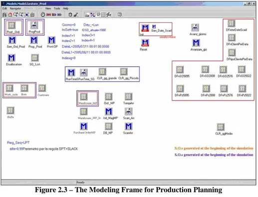
Figure 2.3 – The Modeling Frame for Production Planning “ 36 Figure 2.4 – The Customers’ Orders Inserting Process “ 36 Figure 2.5 – The Inventory Management Process “ 37
Figure 2.6 – The Material Allocation “ 38
Figure 2.7 – The Production Planning “ 38
Figure 2.8 – The Modeling frame for Cutting operations “ 39 Figure 2.9 – Customers’ number per date, empirical distribution “ 40
Figure 2.10 – MSpE Analysis “ 41
Figure 2.11 – Mean Daily Production for Assembly Operation (real and
simulated) “ 42
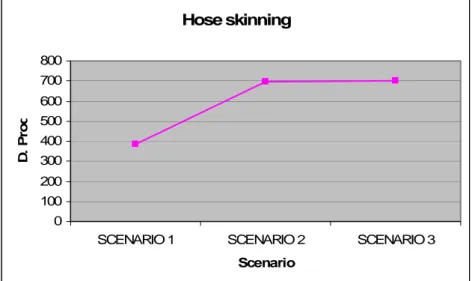
Figure 2.12 – Utilization Degree for Final Controls Operations “ 45 Figure 2.13 – Daily Production for hoses skinning Operations “ 45 Figure 2.14 – The Simulation Model Animation “ 47 Figure 2.15 – Weekly Costs before and after Ants Theory Optimization “ 51 Figure 2.16 – Annual Costs before and after Ants Theory Optimization “ 51 Figure 2.17 – Weekly Costs before and after GA Optimization “ 52 Figure 2.18 – Weekly Costs Comparison between Ants Theory and GA results for
8 Generations “ 53
Figure 2.19 – Weekly Costs Comparison between Ants Theory and GA results for
10 Generations “ 53
Figure 2.20 – Weekly Costs Comparison between Ants Theory and GA results for
12 Generations “ 54
Figure 3.1 – The conceptual model of the system “ 63 Figure 3.2 – Average on-hand inventory versus demand intensity “ 67 Figure 3.3 – Average on-hand inventory versus demand variability “ 68 Figure 3.4 – Average on-hand inventory versus lead time “ 68 Figure 3.5 – Average on-hand inventory for sQ-sS policies “ 70
Figure 3.8 – Mean daily production for different lead times “ 71 Figure 3.9 – The conceptual model of the Supply Chain “ 72 Figure 3.10 – Block diagram for the manufacturing plant selection “ 74 Figure 3.11 – The Distribution Centers Block diagram “ 75
Figure 3.12 – The Stores Block diagram “ 76
Figure 3.13 – The MSpE Analysis “ 77
Figure 4.1 – The Real Warehouse Layout “ 86
Figure 4.2 – The WILMA Simulation Model Flow Chart “ 88
Figure 4.3 – An example of Java code “ 88
Figure 4.4 – The GUI (Input Section) “ 89 Figure 4.5 – The Output Section “ 90 Figure 4.6 – The Full Factorial Experimental Design “ 91 Figure 4.7 – The Pareto Chart for the APDD “ 93 Figure 4.8 – The Most Significant Effects for the ADCP “ 96
Figure 4.9 – ADCP versus Main Effects “ 98
Figure 4.10 – Interactions Plots for the ADCP “ 98 Figure 4.11 – The Pareto Chart for the STWT “ 99 Figure 4.12 – The Normal Probability Plot for the RTWT “ 101 Figure 4.13 – Main Effects Plots for RTWT “ 102 Figure 4.14 – Cube Plot for RTWT “ 102 Figure 4.15 – Response Surfaces for RTWT “ 103
Table 2.I – Utilization Degrees for each scenario Pag.44 Table 2.II – Daily production for each scenario “ 44 Table 3.I – Scenarios Definition “ 65 Table 3.II – Factors and levels for inventory control policies comparison along the
supply chain “ 78
Table 3.III – Fill rate comparison (for each inventory control policy) under
different demand intensity “ 79
Table 3.IV – On-hand inventory comparison (for each inventory control policy)
under different demand intensity “ 79 Table 3.V – Fill rate comparison (for each inventory control policy) under
different demand variability “ 80
Table 3.VI – On-hand inventory comparison (for each inventory control policy)
under different demand variability “ 80 Table 3. VII – Fill rate comparison (for each inventory control policy) under
different demand variability “ 80
Table 3. VIII – On-hand inventory comparison (for each inventory control policy)
under different demand lead times “ 81
Table 4.I – Factors and Levels of DOE “ 91 Table 4. II – Design Matrix and Simulation Results (APDD) “ 94 Table 4.III – ANOVA Results for the APDD (most significant factors) “ 95 Table 4.IV – Design Matrix and Simulation Results (ADCP) “ 97 Table 4.V – ANOVA Results for Significant Factors “ 99 Table 4.VI – ANOVA Results for the most significant factors “ 101
Introduction
This Thesis presents the results of the activities carried out during the three years PhD course at the Mechanical Department of the University of Calabria (Italy), Industrial Engineering Section. The PhD course focuses on the Inventory and Warehouse Management problem in Production Systems and Supply Chain by using advanced investigation approaches based on Modeling & Simulation.
The first step of the PhD course was to correctly define the research area: after an initial pre‐screening of the literature and according to the ongoing research activities at the Modeling & Simulation Center – Laboratory of Enterprise Solutions (MSC‐LES, at Mechanical Department of University of Calabria) it was decided to focus on two specific and related issues: the Inventory Management problems (definition, testing and comparison of new inventory control policies) and the Warehouse Management problem (warehouse resources allocation for improving warehouse internal efficiency and service level provided upstream and downstream the supply chain).
The PhD course has been subdivided into three parts: review of the state of the art, training activities and the research activities.
An accurate review of the state of the art was carried out in the area of Inventory and Warehouse Management: all the academic books, international journals articles and conference proceedings articles reported in the bibliography at the end of each Chapter (and cited within it) have been read, deeply analyzed and discussed. Chapter 1 provides the reader with an accurate overview on methodologies and scientific approaches proposed (during the last decades) by researchers, scientists and practitioners working in the Inventory and Warehouse Management areas. Chapter 1 passes through the description of several research works, as they run through the literature, according to the methodology or scientific approach they propose. The initial search identifies a huge number of references (about 600 references) which were reduced to about 157 references based on contents and quality (112 references cited in Chapter 1 and 45 references in the remaining chapters). The descriptive analysis of the literature reveals heterogeneity among the scientific approaches due to the different models, techniques and methods adopted for facing the inventory and warehouse management problem both in manufacturing systems and in supply chains.
The main goal of training activities was twofold: (i) to learn the main principles to carry out a simulation study and (ii) to gain knowledge and experience in using different simulation software tools to develop simulation models in manufacturing and supply chain areas. Detailed studies have been
made concerning simulation modeling principles, input data analysis, Verification, Validation and Accreditation (V&VA), simulation runs planning by using the Design of Experiments (DOE), simulation results analysis by using the Analysis of Variance (ANOVA). The software tools adopted for the implementation of simulation models and simulation results analysis are: eM‐ Plant™ by Tecnomatix Technology (a discrete event simulation software), Anylogic™ by XJ Technologies (a java‐based simulation software), Minitab™ by
Minitab Inc. (a specific tool for statistical analysis), C++, Simple ++ and Java
(general purpose and specific programming languages for simulation models development). The training activity has been carried out at University of Calabria (MSC‐LES, Industrial Engineering Section) and at General Electric, Oil & Gas Section (Nuovo Pignone S.p.A plant located in Vibo Valentia, Italy). The results of the training part are presented and discussed in Chapter 2. Indeed Chapter 2 presents two applications examples (in two different areas, manufacturing and supply chain) with the aim of facing the main problems and critical issues in developing a simulation study. The application examples developed in this part were useful to gain confidence with simulation and statistic software as well as they also propose (i) an advanced modeling approach for developing flexible and time efficient simulation models and (ii) the integration of two different artificial intelligence techniques (Ants Theory and Genetic Algorithms) with one of the simulation models proposed in the application examples. Note that the application examples proposed in Chapter 2 are not part of the research activities in the area of Inventory and Warehouse Management; as already mentioned the main goal of the training part was to acquire knowledge and experience in developing simulation models. The main results of the research activity are presented in Chapters 3 and 4 respectively for the Inventory Management and Warehouse Management.
Chapter 3 proposes and defines six new inventory control policies. For each inventory control policy a mathematical model is presented. To provide relevance on the potentials of the inventory control policies proposed, their behaviors and performances have been tested and compared in two different real contexts: a manufacturing system devoted to produce high pressure hydraulic hoses and a three echelons supply chain operating in the beverage sector. In both cases an advanced simulation model is used for investigating and comparing inventory control policies behavior under different constraints in terms of demand intensity, demand variability and lead times.
In Chapter 4, after an introduction on the role of warehouses in logistic systems, the warehouse management problem is faced from the point of view of optimal warehouse resources allocations and internal logistics costs reduction. The main goal of the research is to understand how different
warehouse resources allocations affect both the internal warehouse efficiency and the service level provided upstream (suppliers) and downstream (retailers) the supply chain. To this end a simulation model of a real warehouse supporting the large scale retail sector is presented. The first analysis, carried out by using the simulation model, considers the effects of resources allocation on the average number of handled packages per day and on the average daily cost for each handled package. The second analysis evaluates the analytical relationship between some critical parameters (the number of suppliers’ and retailers’ trucks per day, the number of forklifts and lift trucks, the number of warehouse shelves levels) and the service level provided to suppliers and retailers (in terms of waiting time of suppliers’ trucks before starting unloading operations and waiting time of retailers’ trucks before starting loading operations).
The research activities proposed in Chapters 3 and 4 has been developed at University of Calabria (MSC‐LES, Industrial Engineering Section, Italy), at University of Genoa (Savona Campus, DIPTEM and Simulation Team, Italy) and at General Electric, GE Oil & Gas (Nuovo Pignone S.p.A plant, Vibo Valentia, Italy).
C
HAPTER
1
Inventory and Warehouse Management: the state
of art overview
1.1 Introduction on Inventory Management
According to Simchi‐Levi et al. (2007), a Supply Chain (SC) is a network of different entities or nodes (industrial plants, distribution centers (DCs), warehouses and retailers) that provide materials, transform them in intermediate or finished products and deliver them to customers to satisfy market requests.
For characterizing each SC node, two different parameters have to be introduced: • the demand; • the productive capacity. The definition of these parameters usually requires a huge effort in terms of data collection. In effect, the information management related to demand and productive capacity is a very complex task characterized by a great number of critical issues related to: • market needs (volumes and production ranges); • industrial processes (machines downtimes, transportation modes); • supplies (parts quality, delivery schedules). The market demand and the productive capacity also generate a flow of items and finances towards and from the SC node. Needless to say, the Supply Chain Management (SCM) takes care of the above‐mentioned issues, studying and optimizing the flow of material, information and finances along the entire SC. In fact, the main goal of a SC manager is to guarantee the correct flows of goods, information and finances throughout the SC nodes for assuring the right goods in the right place and at the right time. Among others, the inventory management problem along the SC plays a critical role because it strongly affects the SC performances. Lee and Billington (1993) consider the inventory control as the only tool to protect SC stability and robustness. Longo and Ören (2008) also assert that an efficient inventory management along the SC positively affects the SC resilience. In effect, the objective of the Supply Chain Inventory Management (SCIM) is to satisfy the ultimate customer demand increasing quality and service level and decreasing, at the same time, total costs; inventories affect SC costs and performance in terms of:
• values tied up, e.g., raw materials have a lower value than finished products;
• degrees of flexibility, e.g., raw materials have higher flexibility than finished products because they can be easily adopted for different production processes;
• levels of responsiveness, e.g., in some cases products delivery could be made without strict lead times whereas raw materials transformation usually requires stringent lead times.
1.2 The Inventory Management problem
According to Bassin (1990), an efficient inventory control plays a key‐role in the management of each company. In fact, many companies reducing their investments in fixed assets (i.e. plants, warehouses, equipment and machinery) aim also at reducing inventories (Coyle et al., 2003). In particular, wholesalers and retailers have to solve the inventory management problem by keeping inventory at reasonable levels due to the difficulty of demand forecasting and customers’ expectations about products availability (Coyle et
al., 2003).
The difficulty of demand forecasting lead to two opposite issues: the inventory over‐stock and stock‐out. In fact, trying to avoid lost sales caused by inventory stock‐outs, companies demonstrate a tendency to overstock; from the other side, because of the fact that keeping inventory is costly, companies reduce the inventory level, so the tendency to inventory stock‐out is evident. Coyle et al. (2003) argue about the effects of stock‐out while Toomey (2000) discusses about the reasons for setting safety stocks. Goldsby et al. (2005) introduce a new parameter to monitor the inventory levels of a company. This parameter is represented by the inventory turns which can be expressed mathematically as the ratio between the sales volume at cost and the value of average inventory.
As a matter of fact, the Inventory Management problem must address two critical questions:
• time for ordering;
• quantities to be ordered.
According to Minner (2000), addressing correctly such issues also depends on transaction, safety and speculation. The transaction is the result of the fact that ordering and manufacturing decisions are made at certain points of time instead of being performed continuously; the safety emerges in uncertainty situations where lead‐time, demand and production are unknown
at the time of decisions; the speculation is generally related to prices uncertainty.
Furthermore, Minner (2000), groups inventories into:
• cycle stocks: the cycle stock is induced by batching and changes
between an upper level (when a batch has just arrived) and a lower level (just before the arrival of the next batch);
• pipeline stocks: order processing times, production, transportation rates contribute to pipeline stocks, also called process inventories. Material that are in process, in transport, and in transit to another processing unit belong to pipeline stocks;
• safety stocks: the safety stock can be considered as the expected
inventory just before the next replenishment arrives and it is caused by the uncertainty of demand, processing time, production and other factors;
• speculative stocks: they are generated by earlier supplies due to
expected price increase or by possible higher selling prices;
• anticipation stocks: anticipation stocks are related to products with
seasonal demand.
In function of the classification above mentioned, it is difficult to identify to which of the categories a certain item belongs because of stocks can be originated from more than a single inventory control.
1.3 The Inventory Control Systems
According to Silver et al. (1998), an inventory control system has to solve the following three issues: • how often the inventory status should be determined; • when a replenishment order should be placed; • how large the replenishment order should be.These issues become easy to solve under conditions of deterministic demand, but the answers are more difficult to obtain under probabilistic demand.
Literature proposes many inventory control systems and control policies. Most of them deal with some complex mathematical model (Lin, 1980). In the following Sections, the most important inventory control systems are introduced.
1.3.1 The ABC classification
According to Silver et al. (1998), the ABC analysis is an important tool which help company managers to establish how critical the item under
consideration is to the firm. It is an inventory classification technique in which the items in inventory are classified according to the dollar volume (value) generated in annual sales (Fuerst, 1981). Onwubolu and Dube (2006) assert that only the application of the ABC analysis to an inventory situation determines the importance of items and the level of control placed on the items. Furthermore, the A items represent about the 20 percent of the total number of items and the 80 percent of the dollar sales volume; B items are roughly 30 percent of the items, but represent 15 percent of the dollar volume; C items comprise roughly 50 percent of the items, and represent only 5 percent of the dollar volume. Slow‐moving and inexpensive items critical to the company are also included among the A items.
1.3.2 Continuous and periodic review
Once the importance of an item is determined, the next step is to define a control system or policy to monitor inventory status, place replenishment orders for items, decide the amount to be ordered. In the next Section, continuous and periodic review control policies are presented.
Two review approaches can be adopted: the continuous review and the
periodic review. In the first case, the stock status is always known. In reality,
the continuous review is generally not required because in correspondence of each order an immediate updating of the inventory status is made. From the other side, the periodic review implies a definition of the stock status only every R time units, where R is the review interval which is the time that elapses between two consecutive moments at which the stock level is known.
The periodic review system has the advantage to allow a significant prediction of the workload level of the staff involved. From the other side, the continuous review is generally more expensive in terms of reviewing costs and reviewing errors than the periodic review, e.g. fast‐moving items where there are many transactions per unit of time. On the other hand, periodic review is more effective than continuous review in detecting spoilage (or pilferage) of such slow‐moving items. Taking into consideration the customer service level, the continuous review has the advantage to guarantee the same service level with less safety stock than the periodic review because in the case of the periodic review a greater safety protection is needed in order to prevent unexpected reductions of the stock level.
As already mentioned, according to the Supply Chain Inventory Management (SCIM) principles, the objective of an inventory control system is twofold:
• evaluation of the time for purchasing order emission; • evaluation of the quantity to be ordered.
In the following, four classical inventory control policies are described. These policies are: 1. the Re‐Order‐Point, Order Quantity (s, Q) policy; 2. the Periodic‐Review, Order‐Up‐To‐Level (R, S) policy; 3. the Order‐Point, Order‐Up‐To‐level (s, S) policy; 4. the (R, s, S) policy.
The parameter to take into consideration is the Inventory Position (IP) defined as the on‐hand inventory plus the quantity already on order minus the quantity to be shipped. According to Sylver et al. (1998), this parameter has an important role because it includes not the net stock, but the on‐order stock, takes into account all the material ordered but not yet received from the supplier.
In fact, if the net stock is the parameter chosen for deciding when an order should be submitted, unnecessarily another order might be placed today even though a large shipment was due in tomorrow. Next Section presents the mathematical formulation for each policy. 1.3.3 The Re‐Order‐Point, Order‐Quantity (s, Q) policy This is a continuous review system (R = 0). A fixed quantity Q is ordered whenever the inventory position drops to the reorder point s or lower. Note that the inventory position, and not the net stock, is used to trigger an order.
The quantity to be ordered can be defined using the Economic Order Quantity (EOQ) approach.
This control policy is also defined as a two‐bin policy: there are two bins for storage of an item. Demand is initially satisfied from the first bin; when it is used up the second bin is opened so an order is made out for replenishment (the items in the second bin represents the reorder point). When the replenishment arrives, the second bin is refilled and the items been left are put into the first bin. It is important to underline that this system works well when no more than one replenishment order is placed. The advantages of this policy are: • it is simple to adopt, especially in the two‐bin form; • errors are less likely to occur; • predictable production requirements for the supplier. From the other side, the most important disadvantage is related to the incapability, in case of large transactions, to guarantee a quantity large enough to raise the inventory position above the reorder point.
1.3.4 The Periodic‐Review, Order‐Up‐To‐Level (R, S) policy
Unlike the previous control policy, the Periodic‐Review, Order‐Up‐To‐ Level (R,S) policy, also known as a replenishment cycle policy, is based on a periodic check, see Figure 1.1. If R is the review period, every R units of time, the quantity to order is defined by S(t) minus IP(t). The value of R can be defined using the inverse formula usually used for evaluating the EOQ. In this policy, S(t) represents the target level. This policy should be used when: • inventory level is not automatically monitored; • there are advantages related to scale economy; • orders are not regular. Because of its properties, this policy is more adopted than the Re‐Order‐ Point, Order‐Quantity policy because of a simple coordination of the replenishments, e.g. the coordination guaranteed by this policy becomes very important in terms of savings if consider that, in case of orders from overseas, in order to keep shipping costs under control, generally a shipping container is filled. This policy has the main disadvantage that the carrying costs are higher than in continuous review systems. 1.3.5 The Order‐Point, Order‐Up‐To‐Level (s, S) policy
This policy can be derived from the previous policies above mentioned. Like the Re‐Order‐Point, Order‐Quantity policy, a replenishment is made whenever the IP(t) equals or is lower than the re‐order point, see Figure 1.2.
From the other side, this policy differs from the Re‐Order‐Point, Order‐ Quantity policy because, for increasing the IP(t) to the target level, a variable quantity is anyway ordered. According to literature, there are two parameters which characterize this policy: • s (t), the re‐order level at time t; • S(t), the order‐up‐to‐level or target level at time t.
This policy is also defined as min‐max system because the inventory position, with the exception of some particular cases, is included between the minimum value (the order‐point) and a maximum value (the target level). Moreover, according to Sylver et al. (1998), the total costs of replenishment, carrying inventory and shortage are comparable to the costs of the reorder point‐order quantity policy.
1.3.6 The (R, s, S) policy
This inventory management policy can be considered a combination of the (s, S) and (R, S) policies. A check on the inventory position is made every R units of time. If it is at or below the reorder point s, an order enough to raise it to S is produced. If the position is above s, nothing is done until the next review.
Moreover, the (s, S) policy is the special case where R = 0 and the (R, S) is the special case where s = S‐1. From the other side, the (R, s, S) policy can be considered as a periodic version of the (s, S) policy and the (R, S) situation can be viewed as a periodic implementation of (s, S) with s = S‐1.
Scarf (1960) asserts that, under quite general assumptions about the demand pattern and the cost factors involved, the (R, s, S) policy generates lower total replenishment, carrying, and shortage costs than any other inventory control methodologies. However, this policy needs a heavy computational effort because three control parameters have to be evaluated.
Figure 1.1 – The (R,S) policy (Source: Sylver et al. (1998))
Figure 1.2 – The (s,S) policy (Source: Sylver et al. (1998))
1.4 Inventory management research studies
In recent years, a great number of research studies on SCIM have been proposed. In particular, these research studies concern to:
• Analytical models for inventory management. D’Esopo (1968) proposes a review of the re‐order point order‐quantity policy introducing a new time parameter, the expedited lead time, lower than the normal procurement lead time. Ramasesh et al. (1991) propose a variant of the same policy with parameters related to demand variability and lead times to minimize total purchasing, delivery and inventory costs. Cormier and Gunn (1996) discuss about cost models for inventory and inventory sizing models. Minner et al. (1999) consider an analytical model of a two‐echelon system in which parameters related to outstanding orders are introduced; Minner (2003) provides a
review on Inventory Models (IMs) and addresses their contribution to SC performance analysis.
• Constrained inventory management systems. Inderfurth and Minner (1998) investigate an analytical model to determine safety stocks considering as constraint different service levels; Chen and Krass (2001) propose a new inventory approach, based on the minimal service‐level constraint, which consists in achieving a minimum defined service level in each period; Huang et al. (2005) study the impact of the delivery mode on a one‐warehouse multi‐retailer system to evaluate the optimal inventory ordering time and the economic lot size for reducing total inventory costs; De Sensi et al. (2008) propose the analysis of different inventory control policies under demand patterns and lead time constraints in a real SC; Longo and Mirabelli (2008) analyze the effects of inventory control policies, lead times, customers’ demand intensity and variability on three different SC performance measures.
• Inventory management and parameters variability. Moinzadeh and Nahmias (1988) analyze an extension of the classical (s,Q) policy; Moinzadeh and Schmid (1991) study a one‐for‐one ordering policy introducing parameters related to net inventory and the timing of all outstanding orders; Qi et al. (2004) analyze deviation costs of one supplier‐one retailer system after demand disruption; Zhou et al. (2007) introduce an algorithm to compute the parameters of a single item‐periodic review inventory policy.
• Inventory management and SC configurations (single/multi‐echelon
systems). Moinzadeh and Aggarwal (1997) study a multi‐echelon
system incorporating the emergency ordering mechanism; Ganeshan (1999) studies a continuous‐review, one‐warehouse, multiple‐retailer distribution system; Dellaert and De Kok (2004) present an integrated approach for resource, production and inventory management of an assembly system; Chen and Lee (2004) implement an analytical model for demand variability, delivery modes, inventory level and total costs in a multi‐echelon SC network.
• Modelling and simulation for inventory management along the Supply
Chain. The evaluation of the performances of different entities
involved in the SC, from suppliers to final customers passing through DC, involves a number of stochastic variables and parameters and is a quite complex task in which analytical models often fall short of results applicability. The literature analysis show that the Modeling & Simulation (M&S) approach is able to recreate the whole complexity
of a real supply chain. Bhaskaran (1998) carries out a simulation analysis of SC instability and inventory related to a manufacturing plant: in this case, simulation is used in combination with artificial intelligence techniques (i.e., fuzzy theory and genetic algorithms) for a better understanding of the effects of different inventory strategies on the SC structure and for supporting the decision‐making process. Giannoccaro and Pontrandolfo (2002) propose an artificial intelligence algorithm to manage inventory decisions at all SC stages (optimizing the performance of the global SC by using a simulation approach). Huang et al. (2005) solve the ordering and positioning retailer inventories problem at the warehouse and stores, satisfying specific customer demand and minimizing total costs by using neural network approaches. For simulation models development, different commercial software and programming languages have been adopted: Bertazzi et al. (2005) implement in C++ a vendor‐managed inventory policy to minimize purchasing, replenishment and delivery total costs; Lee and Wu (2006) model the reorder point‐order quantity (RPOQ) and the periodic review order‐up policy of a distribution system by using the commercial package eM‐Plant™ while Al‐Rifai and Rossetti (2007) adopt Arena™ for testing a new analytical model for a two‐echelon inventory system.
1.5 Introduction on Warehouse Management
Warehouses are usually large plain buildings used by exporters, importers, wholesalers, manufacturers for goods storage. Warehouses are equipped with loading docks to load and unload trucks, cranes and forklifts for moving goods, as shown in Figure 1.3.
Figure 1.3 – The Warehouse Layout (Source: Rajuldevi et al. (2009))
Some warehouses are fully automated, i.e. products are moved from one place to another by automated conveyors and automated storage and retrieval machines which run by programmable logic controllers and also with logistics automation software (Eben‐Chaime and Pliskin, 1997). This kind of warehouses are characterized by a Warehouse Management System (WMS), a database driven computer program for the material tracking (Mason et al., 2003). As a consequence, logistics experts adopt the WMS to improve the efficiency of the warehouse through an accurate control of the inventory levels.
According to Rajuldevi et al. (2009), during the last years Just in Time (JIT) techniques designed to enhance the return on investment (ROI) of a business by reducing in‐process inventory cause some changes in the traditional warehousing. JIT is based on delivering products directly from manufacturing plants to retailers without using warehouses, but, because of the distance between manufacturers and retailers increases considerably in many regions or countries, a warehouse per region or per country for a given range of products is usually needed (Tompkins et al., 1998).
Nowadays, new changes in marketing strategies are leading to the development of a new warehouse designing approach, i.e. the same warehouse is used for warehousing and also as a retail store. As a consequence, manufacturers can directly reach consumers by avoiding or by‐ passing importers or other middle agencies (Tompkins et al., 1998).
These warehouses are equipped with tall heavy industrial racks where items ready for sale are placed in the bottom parts of the racks while the palletized and wrapped inventory items are usually placed in the top parts. 1.5.1 Warehouses classification
In function of products managed, warehouses can be classified into:
• raw material and components warehouses: they hold raw material and have usually the function to provide raw material to manufacturing or assembly processes;
• work‐in‐process warehouses: they hold partially completed products and assemblies at various points along production lines or assembly lines;
• finished goods warehouses: they are usually situated near the manufacturing plants and hold finished items;
• distribution warehouses/distribution centers: distribution warehouses collect products from various manufacturing points in order to combine shipments to the common customer. Normally, these
warehouses are located at a central position between the manufacturing plants and the customer;
• fulfillment warehouses/fulfillment centers: they receive, pick and ship small orders for individual consumers;
• local warehouses: they receive, pick and ship a few items to the customer every day;
• value‐added service warehouses: in these warehouses key product customization activities take place, i.e. packaging, labeling, marking and pricing.
From a geographical point of view, warehouses can be distinguished into: • centralized warehouse: all the warehousing services are concentrated to
one specific warehouse unit which provides services to the whole firm. A centralized approach is characterized by a high control and efficiency of the system and improvement in productivity through balancing, but it has some limitations like high initial costs, customers’ concentration in only certain market sectors, long internal transportation paths in large central warehouses and higher costs for the infrastructure, etc. (Korpela and Tuominen, 1996);
• de‐centralized warehouse: each warehouse is autonomous and independent from its own resources without any major considerations over the remaining units of the network to which it belongs. In this approach each facility identifies its most effective strategy without considering the impact on the remaining facilities. The main characteristics of the decentralized approach are flexibility, service orientation, increase in responsiveness and they provide as good service as the centralized warehouses in terms of customer service level. Limitations are related to lack of centralized control, resources duplication and costs increase (Tompkins et al., 1998; Mulcahy, 1994).
1.5.2 The warehouse functions
All the processes which take place within a warehouse are reported in Figure 1.4. These processes are:
• receiving: this is the setup operation for all other warehousing activities. In particular, receiving materials is a critical process within a warehouse: it will create problems in put away, storage, picking and shipping processes because if inaccurate deliveries and damaged material are allowed into the warehouse then the same have to be shipped. The receiving process can be subdivided into the following
operations: direct shipping, cross‐docking, receiving scheduling, pre‐ receiving and receipt preparation;
• put away: this is the inverse process of the order picking. It can be subdivided into: direct put away, directed put away, batched and sequenced put away, interleaving;
• pallet storage: there are different storage methodologies, i.e. block stacking, stacking frames, single‐deep selective pallet rack, double‐ deep rack, drive‐in rack, drive‐through‐rack, pallet flow rack, push‐ back rack;
• pallet retrieval: the most popular pallet retrieval systems are walk stackers, counterbalance lift trucks, straddle trucks, side loader trucks, hybrid trucks, automated storage and retrieval (ASR) machines;
Figure 1.4 – The Warehouse Functions (Source: www.readymicrosystems.com)
• case picking systems which can be classified into three categories (Briggs, 1978): pick face palletizing systems, downstream palletizing systems, direct loading systems;
• unitizing and shipping: these activities are classified as container optimization, container loading, weight checking, automated loading, dock management (Briggs, 1978).
1.5.3 Warehousing costs
• general overhead costs: these costs involve the cost of the space available per cubic square meter and infrastructure and also include the cost for various security devices such as security alarms, auto IDs, etc; • delivery costs are the costs incurred in the distribution of the freight by an outside vendor. These costs include the cost of fuel, insurance and the cost of the delivery trucks;
• labour costs: these costs involve the cost of the labour that perform various operations in the warehouse including receiving incoming goods, entering relevant data into computer systems and administrative duties.
The warehouse costs can also be classified as:
• processing costs: these are costs incurred by various operations and processes carried out in the warehouse such as receiving, storing, picking, packaging and shipping;
• storage costs (handling costs): these are costs incurred to store and handle products and are also known as inventory holding costs.
1.5.4 Warehouse management research studies
This Section proposes a review of the state of art on warehouse management. According to Gu et al. (2007), the warehouse management problem can be tied to five major decisions as illustrated in Figure 1.5:
• defining the overall warehouse structure which consists in analyzing the material flow within the warehouse and in specifying the functional departments and their relationships;
• sizing and dimensioning the warehouse and its departments aim at defining the size and dimension of the warehouse as well as the space allocation of the various warehouse departments;
• defining the detailed layout within each department consists in the detailed configuration within a warehouse department, for example, aisle configuration in the retrieval area, pallet block‐stacking pattern in the reserve storage area, and configuration of an Automated Storage/Retrieval System (AS/RS);
• selecting warehouse equipment means to determine an appropriate automation level for the warehouse and identify equipment types for storage, transportation, order picking and sorting;
• selecting operational strategies defines how the warehouse has to be managed, for example, with regards to storage and order picking, i.e. the choice between randomized storage or dedicated storage,
whether or not to do zone picking and the choice between sort‐while‐ pick or sort after‐ pick, etc.
Figure 1.5 – The Warehouse Management Problem
More in detail, the definition of operational performance measures (in terms of costs, capacity, space utilization and service provided) is fundamental for evaluating the effects of specific decisions. Furthermore, efficient performance evaluation methods, i.e. benchmarking, analytical models and simulation models, can help experts to evaluate several system configurations without any considerable costs.
Different surveys on warehouse management studies are proposed by Cormier (2005), Cormier and Gunn (1992), Van den Berg (1999) and Rowenhorst et al. (2000).
Literature review on warehouse design can be classified into four main topics: • warehouse design (or management); • warehouse performance analysis; • warehousing case studies; • computational (or simulation) models. Now the state of art on warehouse design and management which can be subdivided into five subsections (Figure 1.5) is provided. 1.5.5 The warehouse design and management
As before mentioned, defining the overall structure (or conceptual design) of a warehouse consists in designing the functional departments, i.e. the number of storage departments (Park and Webster, 1989; Gray et al., 1992; Yoon and Sharp, 1996), technologies to adopt (Meller and Gau, 1996), personnel to engage, aiming at satisfying storage and throughput requirements and minimizing costs.
Warehouse sizing and dimensioning has important implications on construction, inventory management and material handling costs. In particular, warehouse sizing establishes the storage capacity of a warehouse. Two scenarios can be considered in solving the sizing problem:
• the inventory level is defined externally and, as a consequence, the warehouse has no direct control on the incoming shipments arrivals and quantities (e.g. in a third‐party warehouse), but the warehouse has to satisfy all the requirements for storage space. White and Francis (1971) study this problem for a single product over a finite planning horizon taking into consideration costs related to warehouse construction, storage of products and storage demand not satisfied within the warehouse;
• the warehouse can directly control the inventory policy as in the case of an independent wholesale distributor so correct inventory policies and inventory costs should be evaluated, see Levy (1974), Rosenblatt and Roll (1988), Cormier and Gunn (1996) and Goh et al. (2001).
The state of art also proposes research studies with either fixed or changeable storage size (i.e. the storage size changes over the planning horizon so the decision variables are the storage sizes for each time period), as reported in Lowe et al. (1979), Hung and Fisk (1984) and Rao and Rao (1998).
From the other side, warehouse dimensioning deals with the floor space definition in order to evaluate construction and operating costs. Francis (1967) faces this problem for the first time by using a continuous approximation of the storage area without considering aisle structure; Bassan et al. (1980) review Francis (1967) model by considering aisle configurations; Rosenblatt and Roll (1984) integrate the optimization model in Bassan et al. (1980) with a simulation model which evaluates the storage shortage cost as a function of storage capacity and number of zones.
Other research studies propose a trade‐off in determining the total warehouse size, allocating the warehouse space among departments, and determining the dimension of the warehouse and its departments, as reported in Pliskin and Dori (1982), Azadivar (1989) and Heragu et al. (2005).
Within each warehouse department, the department layout or storage problem can be classified in:
• pallet block‐stacking pattern (storage lane depth, number of lanes for each depth, stack height, pallet placement angle with regards to the aisle, storage clearance between pallets and length and width of aisles);
• storage department layout (door location, aisle orientation, length and width of aisles and number of aisles); • AS/RS configuration (dimension of storage racks, number of cranes). These layout problems affect warehouse performances in terms of: • construction and maintenance costs; • material handling costs; • storage capacity; • space utilization; • equipment utilization.
Literature proposes several research works related to this issue. A number of papers discuss the pallet block‐stacking problem.
Moder and Thornton (1965) focus on different ways of stacking pallets within a warehouse; Berry (1968) discusses the tradeoffs between storage efficiency and material handling costs through analytic models; Marsh (1979) uses simulation to evaluate the effect on space utilization of alternate lane depths and the rules for assigning incoming shipments to lanes; Marsh (1983) compares the layout design developed by using the simulation models developed in 1979 and the analytic models proposed by Berry (1968). Goetschalckx and Ratliff (1991) develop an efficient dynamic programming algorithm to maximize space utilization while Larson et al. (1997) propose an heuristic approach for the layout problem in order to maximize storage space utilization and minimize material handling cost.
Additional research works on the storage department layout are reported in: Roberts and Reed (1972), Bassan et al. (1980), Roll and Rosenblatt (1983), Pandit and Palekar (1993) and Roodbergen and Vis (2006).
Concerning the AS/RS configuration, some of the papers overviewed are the following: Karasawa et al. (1980) who present a nonlinear formulation with decision variables (i.e. the number of cranes, the height and length of storage racks, construction and equipment costs) under service and storage constraints. Ashayeri et al. (1985) solve a problem similar to Karasawa et al. (1980). Rosenblatt et al. (1993) propose a combined optimization and simulation approach derived from Ashayeri et al. (1985). Malmborg (2001) adopts simulation to evaluate some of the parameters then used in the closed form equations while Randhawa et al. (1991) and Randhawa and Shroff (1995) use simulation to investigate different I/O configurations on performance such as throughput, mean waiting time, and maximum waiting time.
The other topic of warehouse design and management is related to the
equipment selection which has the objective to identify the automation level and
There are a few research works in this field, see Cox (1986) and Sharp et
al. (1994). Operation strategies have important effects on the overall system
and can not be frequently changed. Such strategies concern the decision about different storage ways or decisions to use zone picking. The basic storage strategies include random storage, dedicated storage, class based storage, and Duration‐of‐Stay (DOS) based storage, as explained in Gu et al. (2007). Hausman et al. (1976), Graves et al. (1977) and Schwarz et al. (1978) make a comparison of random storage, dedicated storage, and class‐based storage in single‐command and dual‐command AS/RS using both analytical models and simulations while Goetschalckx and Ratliff (1990) and Thonemann and Brandeau (1998) demonstrate theoretically that the DOS‐based storage policies perform better in terms of traveling costs.
About zone picking approaches, some interesting research works are reported in Lin and Lu (1999), Bartholdi et al. (2000) and Petersen (2000).
1.5.6 The warehouse performance analysis
Performance evaluation approaches, i.e. benchmarking, analytical models and simulation, have the objective to provide information about the quality of a proposed design and/or operational policy in order to improve/to change it.
Warehouse benchmarking is the process of systematically assessing the performance of a warehouse, identifying inefficiencies, and proposing improvements (Gu et al., 2007). A powerful tool for solving this problem is the Data Envelopment Analysis (DEA) which has the capability to capture simultaneously all the relevant inputs (resources) and outputs (performances), to identify the best performance domain and to delete the warehouse inefficiencies. Schefczyk (1993), Hackman et al. (2001) and Ross and Droge (2002) shows some approaches and case studies about using DEA in warehouse benchmarking.
Analytical models can be divided into:
• aisle based models which focus on a single storage system and address travel or service time, see Hwang and Lee (1990), Chang et al. (1995), Chang and Wen (1997), Lee (1997), Hwang et al. (2004b), Meller and Klote (2004), Roodbergen and Vis (2006);
• integrated models which address either multiple storage systems or criteria in addition to travel/service times, as reported in Malmborg (1996), Malmborg and Al‐Tassan (2000).
1.5.7 Warehousing case studies and computational (or simulation) models Some case studies on the applications of the various design and operation methods have been carried out, see Van Oudheusden et al. (1988), Zeng et al. (2002) and Dekker et al. (2004).
Successful research works on the implementation of warehouse computational or simulation models are rare. Perlmann and Bailey (1988) present a computer‐aided design software that allows a warehouse designer to quickly generate a set of conceptual design alternatives including building shape, equipment selection, and operational policy selection, and to select from among them the best one based on the specified design requirements. Linn and Wysk (1990) develop an expert system for AS/ RS control. A similar AS/RS control system is proposed by Wang and Yih (1997) based on neural networks while Ito et al. (2002) propose an intelligent agent based system to model a warehouse, which is composed of three subsystems, i.e. agent‐based communication system, agent‐based material handling system, and agent‐ based inventory planning and control system. Macro and Salmi (2002) present a ProModel‐based simulation tool of a warehouse used for analyzing the warehouse storage capacity and rack efficiency. Finally, Hsieh and Tsai (2006) implement a simulation model for finding the optimum design parameters of a real warehouse system.
1.6 Conclusions
This Chapter reports the results of the state of art overview on the Inventory and Warehouse Management carried out during the first part of the PhD course. More in detail, the state of art analysis on Inventory Management highlights that:
• the classical inventory control policies don’t include stochastic variables;
• literature reports inventory management policies which don’t consider inventory constraints due to demand intensity, demand variability and lead times;
• simulation model implemented are ad‐hoc built simulation models because they reproduce a specific manufacturing system or supply chain.
Moreover, from the state of art analysis on the Warehouse Management becomes clear that research studies on warehouse management simulation are rare and they aim at solving particular problems under constraints (i.e. material flow, size and dimension of the warehouse, warehouse equipment selection, etc).
References
Al‐Rifai, M.H., Rossetti, M.D., 2007. An efficient heuristic optimization algorithm for a two‐echelon (R, Q) inventory system. Production Economics, 109, 195‐213.
Ashayeri, J., Gelders, L., Wassenhove, L.V., 1985. A microcomputer‐based optimization model for the design of automated warehouses. Production
Research, 23 (4), 825‐839.
Azadivar, F., 1989. Optimum allocation of resources between the random access and rack storage spaces in an automated warehousing system.
Production Research, 27 (1), 119‐131.
Bartholdi, J.J., Eisenstein, D.D., Foley, R.D., 2000. Performance of bucket brigades when work is stochastic. Operations Research, 49 (5), 710‐719.
Bassan, Y., Roll, Y., Rosenblatt, M.J., 1980. Internal layout design of a warehouse. AIIE Transactions, 12 (4), 317‐322.
Bassin, W.M., 1990. A Technique for Applying EOQ Models to Retail Cycle Stock Inventories. Small Business Management, 28 (1), 48‐55. Bhaskaran, S., 1998. Simulation analysis of a manufacturing supply chain. Decision Sciences, 29 (3), 633‐657. Berry, J.R., 1968. Elements of warehouse layout. Production Research, 7 (2), 105‐121. Bertazzi, L., Paletta, G., Speranza, M.G., 2005. Minimizing the total cost in an integrated vendor‐managed inventory system. Journal of Euristics, 11, 393‐ 419.
Briggs, J.A., 1978. Warehouse operations planning and management. Krieger Publishing Company, New York.
Chang, D.T., Wen, U.P., Lin, J.T., 1995. The impact of
acceleration/deceleration on travel‐time models for automated