Atmospheric remote sensing and radiopropagation: from numerical modeling to spaceborne and terrestrial applications

(1)

F

I

E

,

I

S

D

EPARTMENT OF

I

NFORMATION

E

NGINEERING

,

E

LECTRONICS AND

T

ELECOMMUNICATIONS

______________________

D

OCTORATE

(P

H

D)

IN

I

NFORMATION AND

C

OMMUNICATIONS

T

ECHNOLOGIES

Atmospheric remote sensing and radiopropagation: from numerical

modeling to spaceborne and terrestrial applications

Candidate Supervisor

Luca Milani Prof. Frank Silvio Marzano

DOCTORATE CYCLE XXXII

(2)

Ai miei fantastici Nonni,

alla mia Famiglia,

agli Amici veri.

(3)

III

Abstract

The remote sensing of electromagnetic wave properties is probably the most viable and fascinating way to observe and study physical media, comprising our planet and its atmosphere, at the same time ensuring a proper continuity in the observations. Applications are manifold and the scientific community has been importantly studying and investing on new technologies, which would let us widen our knowledge of what surrounds us. This thesis aims at showing some novel techniques and corresponding applications in the field of the atmospheric remote sensing and radio-propagation, at both microwave and optical wavelengths.

The novel Sun-tracking microwave radiometry technique is shown. The antenna noise temperature of a ground-based microwave radiometer is measured by alternately pointing toward-the-Sun and off-the-Sun while tracking it along its diurnal ecliptic. During clear sky the brightness temperature of the Sun disk emission at K and Ka frequency bands and in the under-explored millimeter-wave V and W bands can be estimated by adopting different techniques. Parametric prediction models for retrieving all-weather atmospheric extinction from ground-based microwave radiometers are tested and their accuracy evaluated. Moreover, a characterization of suspended clouds in terms of atmospheric path attenuation is presented, by exploiting a stochastic approach used to model the time evolution of the cloud contribution.

A model chain for the prediction of the tropospheric channel for the downlink of interplanetary missions operating above Ku band is proposed. On top of a detailed description of the approach, the chapter presents the validation results and examples of the model-chain online operation. Online operation has already been tested within a feasibility study applied to the BepiColombo mission to Mercury operated by the European Space Agency (ESA) and by exploiting the Hayabusa-2 mission Ka-band data by the Japan Aerospace Exploration Agency (JAXA), thanks to the ESA cross-support service. A preliminary (and successful) validation of the model-chain has been carried out by comparing the simulated signal-to-noise ratio with the one received from Hayabusa-2.

At the next ITU World Radiocommunication Conference 2019, Agenda Item 1.13 will address the identification and the possible additional allocation of radio-frequency spectrum to serve the future development of systems supporting the fifth generation of cellular mobile communications (5G). The potential impact of International Mobile Telecommunications (IMT) deployments is shown in terms of received radio frequency interference by ESA’s telecommunication links. Received interference can derive from several radio-propagation mechanisms, which strongly depend on atmospheric conditions, radio frequency, link availability, distance and path topography; at any time a single mechanism, or more than one may be present. Results are shown in terms of required separation distances, i.e. the minimum distance between the earth station and the IMT station ensuring that the protection criteria for the earth station are met.

(4)

IV

Finally a novel remote sensing technique applied to optical wavelengths is presented, consisting of an anomaly detection and estimation method, using a pixel-based modified version of the Kalman temporal filter. In order to detect anomalies of the observed variable, the proposed Kalman-based anomaly masking (KAM) algorithm relies on background state models of the expected measurement cycle of each pixel in nominal (abnormal) conditions. If the measurement significantly deviates from its expected value as predicted by a-priori state, an anomaly is identified. The algorithm also provides an a-priori estimate of the nominal scenario, exploiting the previous Kalman filter states. The product is an equivalent clear-air observation, expected to be measured in absence of anomaly (e.g., in absence of cloud coverage). The KAM algorithm exhibits a general applicability, since its estimates are empirically computed from pixel-based models and its thresholds can be set independently from the area of interest. An application of the KAM algorithm to clear-air nominal scenarios is shown using multispectral imagery from the geostationary Spinning Enhanced Visible and Infrared Imager, having 12 visible-infrared channels and repeat cycle of 15 minutes, on-board of the Meteosat Second Generation satellite.

(5)

V

Acknowledgments

First, I would like to sincerely thank my supervisor, Professor Frank Marzano, for his continuous support and all the enormous passion he has passed on to me, from both a professional and a human perspective.

I also want to thank everyone I have been working with for the last years, especially all the colleagues of the Sapienza University of Rome, CETEMPS University of L’Aquila, Progressive Systems, and the European Space Agency. The list would be huge and I am very glad I had the chance to interact with so many valuable and competent people: all of this would not have been possible without you.

(6)

VI

Headlines

ABSTRACT ... III ACKNOWLEDGMENTS ... V

CHAPTER 1. INTRODUCTION ... 1

CHAPTER 2. ATMOSPHERIC REMOTE SENSING AND PROPAGATION FUNDAMENTALS ... 4

CHAPTER 3. GROUND-BASED MICROWAVE RADIOMETRY FOR EARTH-SATELLITE ATTENUATION RETRIEVAL ... 25

CHAPTER 4. MODEL-BASED PREDICTION OF DATA RATE FOR DEEP-SPACE SATELLITE MISSIONS ... 49

CHAPTER 5. MICROWAVE INTERFERENCE SOURCE MODELLING AND TERRESTRIAL APPLICATIONS ... 63

CHAPTER 6. CLEAR-SKY DYNAMICAL DETECTION FROM GEOSTATIONARY INFRARED IMAGERY ... 76

CHAPTER 7. CONCLUSIONS ... 97

REFERENCES ... 100

APPENDICES ... 111

(7)

VII

List of figures

FIGURE 2-1:REAL (ϵR) AND IMAGINARY (ϵJ) PARTS OF RELATIVE PERMITTIVITY OF AIR AT STANDARD CONDITIONS MODELED [7] AS A FUNCTION OF MICROWAVE FREQUENCY F (DIAGRAM FROM [1]) ... 7

FIGURE 2-2:ATMOSPHERIC OPACITY FOR U.S. STANDARD ATMOSPHERE WITH LIQUID AND ICE WATER CLOUDS.THE ICE WATER CONTRIBUTION IS BELOW 0.01NP THROUGHOUT THE 10-100GHZ RANGE.THE SPECTRAL RANGE OF COMMERCIALLY AVAILABLE WATER VAPOR (WV;K-BAND 20-30GHZ) AND TEMPERATURE (V-BAND 50-60GHZ) MICROWAVE PROFILERS IS INDICATED (FIGURE FROM [20]). ... 12

FIGURE 2-3:SCHEMATIC VIEW OF A MULTI-FREQUENCY HETERODYNE MICROWAVE RECEIVER.LOW NOISE AMPLIFIERS (LNA) ARE IMPLEMENTED IN THE RADIO FREQUENCY (RF) AND INTERMEDIATE FREQUENCY (IF).AFTER THE SIGNAL SPLITTING BAND PASS FILTERING, AMPLIFICATION AND DETECTION TAKES PLACE IN THE INDIVIDUAL CHANNELS.THE ANALOGUE SIGNALS ARE COMBINED BY A MULTIPLEXER (MUX) AND CONVERTED BY ANALOGUE DIGITAL CONVERTERS (ADC) TO DIGITAL COUNTS (FIGURE FROM [20]). ... 14

FIGURE 2-4:DETECTOR RESPONSE AS A FUNCTION OF INPUT NOISE T.TC IS THE TOTAL NOISE WHEN THE RADIOMETER IS TERMINATED WITH A COLD LOAD (E.G. LIQUID NITROGEN COOLED ABSORBER) AND _TH THE CORRESPONDING NOISE TEMPERATURES FOR THE AMBIENT LOAD,TN THE ADDITIONALLY INJECTED NOISE... 16

FIGURE 2-5:LONG-TERM INTERFERENCE PROPAGATION MECHANISMS (IMAGE FROM [61]) ... 21

FIGURE 2-6:ANOMALOUS (SHORT-TERM) INTERFERENCE PROPAGATION MECHANISMS (IMAGE FROM [61]) ... 21

FIGURE 2-7:SPECTRAL REFLECTANCE CHARACTERISTICS OF COMMON EARTH SURFACE MATERIALS IN THE VISIBLE AND NEAR-TO-MID INFRARED RANGE.1=WATER,2=VEGETATION,3=SOIL.THE POSITIONS OF SPECTRAL BANDS FOR COMMON REMOTE SENSING INSTRUMENTS ARE INDICATED (IMAGE FROM [3]). ... 22

FIGURE 2-8:ENERGY FROM PERFECT RADIATORS (BLACK BODIES) AS A FUNCTION OF WAVELENGTH (IMAGE FROM [3]). ... 23

FIGURE 3-1:ST-MWR OPERATION: THE RADIOMETER TRACKS THE SUN DURING ITS MOTION CONSIDERING A CONSTANT ELEVATION ANGLE Θ BETWEEN TWO CLOSE MEASUREMENTS TAKEN VARYING THE AZIMUTH FROM TOWARD-THE-SUN Φ1 TO OFF-THE-SUN Φ2... 27 FIGURE 3-2:TIME SERIES OF ST-MWR MEASUREMENTS IN TERMS OF ANTENNA NOISE TEMPERATURES FOR A CASE STUDIES REFERRING TO A

CLEAR AIR (OCTOBER 10,2015) AT THE 4AFRL-MWR AVAILABLE FREQUENCIES: A)23.8 AND 31.4GHZ; B)72.5 AND 85.5GHZ.

... 36 FIGURE 3-3:APPLICATION OF THE LANGLEY TECHNIQUE TO ESTIMATE TBSUN*(128 SAMPLES EQUALLY SPACED IN TERMS OF AIR MASS), AS

DISCUSSED IN SECT.II.B, FOR EACH FREQUENCY ON OCTOBER 10,2015: A)23.8(R2=0.9367) AND 31.4GHZ (R2=0.9630); B)

72.5(R2_=0.9984)_AND_85.5_GH_Z_(R2_{=0.9909). ... 37}

FIGURE 3-4:ESTIMATES OF _TBSUN* USING THE METEOROLOGICAL TECHNIQUE FOR EACH FREQUENCY ON OCTOBER 10,2015. ... 37 FIGURE 3-5:TIME SERIES OF ST-MWR MEASUREMENTS IN TERMS OF ANTENNA NOISE TEMPERATURES FOR A CASE STUDIES IN PRESENCE OF

CLOUDS OR PRECIPITATION (29SEPTEMBER 2015) AT THE 4AFRL-MWR AVAILABLE FREQUENCIES: A)23.8 AND 31.4GHZ; B)72.5 AND 85.5GHZ. ... 40

FIGURE 3-6:SCATTERPLOT OF ST-MWR ATMOSPHERIC EXTINCTION FOR EACH FREQUENCY VERSUS EXTINCTION ESTIMATES FROM

PPM-POLDEX FOR ALL CLOUDY/RAINY CONDITIONS. ... 43

FIGURE 3-7:PROBABILITY DENSITY FUNCTION (PDF) AND CUMULATIVE DISTRIBUTION FUNCTION (CDF), INTER-COMPARISON BETWEEN REAL MEASUREMENTS AND SIMULATED STOCHASTIC PROCESS ... 48

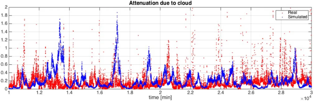
FIGURE 3-8 TIME DOMAIN COMPARISON BETWEEN REAL MEASUREMENTS AND SIMULATED STOCHASTIC PROCESS ... 48

FIGURE 4-1:MODEL CHAIN: WEATHER FORECAST (RED), RADIOPROPAGATION (BLUE) AND DOWNLINK BUDGET (GREEN) MODULES.GREY BLOCKS ARE MEASUREMENTS AND STATISTICS USED FOR TUNING AND VALIDATING THE THREE MODULES. ... 52

FIGURE 4-2:RECEIVING SYSTEM BLOCK-SCHEME. ... 53

FIGURE 4-3:YEARLY LOST (A) AND RECEIVED (B) DATA VOLUME (DV) IN CEBREROS AT KA BAND.NOTE THAT RECEIVED DATA ARE EXPRESSED IN PERCENTAGE WITH RESPECT TO REFERENCE ADVANCED TECHNIQUE (FROM [158]). ... 56

FIGURE 4-4:INNER DOMAIN AND 7X7 PIXELS SUB-GRID (BLUE RECTANGLE) CENTERED ON GROUND-STATION ANTENNA (INDICATED WITH A DIAMOND)... 58

FIGURE 4-5:ES/N0 PROBABILITY DENSITY FUNCTION FOR A GIVEN TEMPORAL INSTANT AND A GIVEN RS VALUE: MEDIAN VALUE (RED) WITH

ERROR-BAR DETERMINED BY ITS 25TH₍_GREEN₎_AND₇₅TH₍_BLUE₎_PERCENTILE_{. ... 58}

FIGURE 4-6:MODEL-CHAIN VALIDATION (AUGUST 11,2018,MALARGÜE) ... 59

FIGURE 4-7:MODEL-CHAIN OPERATION ON NOVEMBER 10,2018,MALARGÜE: OPTIMIZED RS(OPT., GREEN) VS RS ACTUALLY ADOPTED BY

(10)

X

FIGURE 4-8:ATTENUATION TIME-SERIES IN MALARGÜE FOR EACH OF THE 7X7 PIXELS OF THE SUB-GRID DOMAIN (10NOV.2018).PIXEL 1

CORRESPONDS TO MALARGÜE. ... 62

FIGURE 5-1:EXAMPLE OF TERRAIN HEIGHTS MAP AROUND THE MALARGÜE DEEP SPACE STATION IN ARGENTINA ... 65

FIGURE 5-2:IMT-20205G ANTENNA PATTERN AT ZERO TILT (24.25-33.40GHZ) ... 67

FIGURE 5-3:IMT-2020BS(SUBURBAN HOTSPOT)–DEFINITION OF TOTAL TILT ΘTILT TOT ... 69

FIGURE 5-4:SIMULATION EXAMPLE AT 26GHZ FOR AN AZIMUTH CUT AROUND THE MALARGÜE DEEP SPACE STATION IN ARGENTINA (OUTDOOR SUBURBAN IMT DEPLOYMENT, SINGLE ENTRY) ... 73

FIGURE 5-5:SIMULATION EXAMPLE AT 26GHZ –SEPARATION DISTANCES (COORDINATION CONTOUR) AROUND THE MALARGÜE DEEP SPACE STATION IN ARGENTINA (OUTDOOR SUBURBAN IMT DEPLOYMENT, SINGLE ENTRY) ... 74

FIGURE 6-1. DYNAMIC THRESHOLD FUNCTION, EXAMPLE.GRAPHICAL REPRESENTATION OF THE EQUATIONS (6.9) AND (6.10).THE GREEN DOTS CORRESPOND TO THE OBSERVATIONS ZK, THE BLACK CURVE IS THE A-PRIORI ESTIMATE XK- AND THE RED CURVE REPRESENTS THE BACKGROUND MODEL MK.THE GREEN AREA CORRESPONDS TO THE ANOMALY-FREE REGION.A DETAILED DESCRIPTION IS PROVIDED IN THE TEXT.THE LOWER LEFT FIGURE SHOWS AN EXAMPLE OF EQUATION (6.10), USING THE VALUES IN TABLE 6-3 FOR THE IR039 CHANNEL. ... 83

FIGURE 6-2.SCHEME OF THE MULTI-SPECTRAL KALMAN-BASED CLEAR-AIR MASKING (KAM) FILTER.EACH MODULE CORRESPONDS TO A SOFTWARE COMPONENT DEVELOPED FOR NEARLY REAL-TIME APPLICATIONS OF THE ALGORITHM FOR CLEAR-AIR MASKING. ... 86

FIGURE 6-3:EXAMPLE OF CLEAR-AIR DAY (DECEMBER 9,2015) FOR ALL CONSIDERED CHANNELS OF THE MSG-SEVIRI INSTRUMENT.THE GREEN CURVES REPRESENT THE ACTUAL OBSERVATION VECTOR ZK, THE BLACK DOTTED CURVE IS THE A-PRIORI ESTIMATE XK- AND THE RED CURVE REPRESENTS THE BACKGROUND MODEL MK.A DETAILED DESCRIPTION IS PROVIDED IN THE TEXT. ... 91

FIGURE 6-4. EXAMPLE OF “ANOMALY” DAY (DECEMBER 10,2015) FOR ALL CONSIDERED CHANNELS OF THE MSG-SEVIRI INSTRUMENT. THE GREEN CURVES REPRESENT THE ACTUAL OBSERVATION VECTOR ZK, THE BLACK DOTTED CURVE IS THE A-PRIORI ESTIMATE XK- AND THE RED CURVE REPRESENTS THE BACKGROUND MODEL MK.A DETAILED DESCRIPTION IS PROVIDED IN THE TEXT. ... 92

FIGURE 6-5:INTER-COMPARISON WITH RESPECT TO EUMETSATCLOUD MASK PRODUCT FOR A SINGLE TIMESLOT (JANUARY 19,2016 H 12:00).BLUE AND CYAN POINTS CORRESPOND TO PIXELS FOR WHICH THE TWO ALGORITHMS PROVIDE THE SAME RESULT (CLEAR-AIR AND ANOMALY, RESPECTIVELY).YELLOW POINTS REPRESENT MISSED DETECTIONS OF THE KAM ALGORITHM WITH RESPECT TO THE EUMETSAT MASKING PRODUCT, WHILE BROWN PIXELS INDICATE FALSE ALARMS. ... 94

FIGURE 6-6:COMPOSITE RGB IMAGE FROM THE MSG-SEVIRI INSTRUMENT FOR THE CONSIDERED TIMESLOT IN FIGURE 6-5(JANUARY 19, 2016 H 12:00). ... 95

FIGURE 6-7:INTER-COMPARISON (TEMPORAL TREND) BETWEEN THE KAM ALGORITHM AND THE EUMETSATCLOUD MASK PRODUCT OVER THE WHOLE ANALYZED PERIOD FOR ALL PIXELS COMPOSING THE SCENE.BLUE AND CYAN POINTS CORRESPOND TO PIXELS FOR WHICH THE TWO ALGORITHMS PROVIDE THE SAME RESULT (CLEAR-AIR AND ANOMALY, RESPECTIVELY).YELLOW POINTS REPRESENT MISSED DETECTIONS OF THE KAM ALGORITHM WITH RESPECT TO THE EUMETSAT MASKING PRODUCT, WHILE BROWN PIXELS INDICATE FALSE ALARMS. ... 96

FIGURE A-0-1:SENSITIVITY ANALYSIS OF ST-MWR PERFORMANCES FOR A SET OF VALUES WHICH ARE THOSE EXPECTED BETWEEN KA AND W BAND. ... 112

FIGURE B-0-2:TWO NESTED DOMAINS OF THE NWP MODELS CENTERED ON THE TARGET AREA OF ROME,NY:(A) DOMAIN 1 AT 18 KM (AND 9 KM) RESOLUTION;(B): DOMAIN 2 AT 6 KM (AND 3 KM) RESOLUTION. ... 123

FIGURE B-0-3:COMPLEMENTARY CUMULATIVE DISTRIBUTION FUNCTION OF A COMPUTED FROM 3D-RTM SIMULATIONS FROM 1AUGUST 2015 TO 31JULY 2016 FOR THE FREQUENCIES OF INTEREST. ... 124

FIGURE B-0-4:NUMERICAL WEATHER PREDICTIONS VALIDATION WITH RADIOSOUNDING DATA:(A) ABSOLUTE HUMIDITY,(B) TEMPERATURE. ... 125

FIGURE B-0-5:VERTICAL PROFILE OF INDEX OF AGREEMENT BETWEEN WRF AND RADIOSOUNDING DATA FOR ABSOLUTE HUMIDITY AND TEMPERATURE PROFILES. ... 126

FIGURE B-0-6:COMPARISON BETWEEN WRF AND RADAR DATA IN TERMS OF RAIN ACCUMULATED IN 1 HOUR ON A DOMAIN CENTERED ON ALBANY SITE. ... 127

FIGURE B-0-7:TB SCATTERPLOT FOR THE PERIOD FROM 1AUGUST 2015 TO 31JULY 2016:3D-RTM VS ST-MWR AFTER TIME -MATCHING AT ALL ELEVATION ANGLES INTERESTED BY THE ST-MWR MEASUREMENTS. ... 128

FIGURE B-0-8:TB SCATTER DENSITY PLOT FOR THE PERIOD FROM 1AUGUST 2015 TO 31JULY 2016:3D-RTM VS PRO-MWR AFTER TIME-MATCHING AT ZENITH VIEW. ... 130

FIGURE B-0-9:TB-TB CHANNEL CORRELATION OF ST-MWR,1D-RTM AND 3D-RTM AT THE ST-MWR FREQUENCY CHANNELS.ALL THE ELEVATION ANGLES ARE INCLUDED. ... 131

FIGURE B-0-10:TB-A CORRELATION OF ST-MWR,1D-RTM AND 3D-RTM AT THE FOUR ST-MWR FREQUENCY CHANNELS.ALL THE ELEVATION ANGLES ARE INCLUDED. ... 132

(11)

XI

FIGURE B-0-11:TB-TB CHANNEL CORRELATION OF PRO-MWR,1D-RTM AND 3D-RTM AT THE PRO-MWR FREQUENCY CHANNELS,

ZENITH VIEW. ... 132

FIGURE B-0-12:COMPLEMENTARY CUMULATIVE DISTRIBUTION FUNCTION OF A FROM 3D-RTM,1D-RTM, AND ST-MWR, ZENITH VIEW.

ST-MWR MEASUREMENTS HAVE BEEN REPORTED TO THE ZENITH VIA THE COSECANT LAW. ... 133

FIGURE B-0-13:(A)DIVISION OF THE ST-MWR DATASET INTO AIR-MASS INTERVALS AND (B) CORRESPONDING ELEVATION-ANGLES INTERVALS. ... 134

(12)

XII

List of tables

TABLE 3-1:MONTHLY CLASSIFICATION OF CLEAR, CLOUDY AND RAINY DAYS DURING AFRLST-MWR AVAILABLE MEASUREMENTS ... 34

TABLE 3-2:LANGLEY AND METEOROLOGICAL DAILY ESTIMATES OF _{𝑇𝑇𝑇𝑇𝑇𝑇𝑇𝑇𝑇𝑇 ∗ ... 38}

TABLE 3-3:LANGLEY AND METEOROLOGICAL AVERAGE ESTIMATE INTER-COMPARISON ... 39

TABLE 3-4:LANGLEY AND METEOROLOGICAL ESTIMATE DEVIATIONS INTER-COMPARISON ... 39

TABLE 3-5:ATMOSPHERIC EXTINCTION INTER-COMPARISON BETWEEN ST-MWR AND PPM-POLDEX MODEL FOR THE AVAILABLE DATASET IN 2015 IN ROME,NY ALL-WEATHER CASES ... 42

TABLE 3-6:ATMOSPHERIC EXTINCTION INTER-COMPARISON BETWEEN ST-MWR AND PPM-POLDEX MODEL FOR THE AVAILABLE DATASET IN 2015 IN ROME,NY CLOUDY AND RAINY CASES ... 42

TABLE 3-7:PPM-POLDEX MODEL COEFFICIENTS AT 32GHZ ... 45

TABLE 4-1 SYMBOL LEGEND ... 53

TABLE 5-1:ITU-R RECOMMENDED PROTECTION CRITERIA FOR SRS AND EESS EARTH STATIONS ... 65

TABLE 5-2:IMT-2020 CHARACTERISTICS –STATIC PARAMETERS (OUTDOOR SUBURBAN/URBAN HOTSPOTS [169]) ... 68

TABLE 5-3:MAXIMUM COORDINATION DISTANCES FOR THE ESA’S EARTH STATIONS CONSIDERED IN THE COMPATIBILITY STUDIES ... 75

TABLE 6-1:MODIFIED TEMPORAL KALMAN FILTER,SUMMARY OF VARIABLES AND THEIR DEFINITIONS WITH N THE NUMBER OF AVAILABLE OBSERVATIONS SPANNED BY THE INDEXES I=1,…,N; J=1,…,N ... 78

TABLE 6-2:SEVIRINOISE BUDGETS AS MEASURED AT THE BEGINNING OF LIFE, EXPECTED AT THE END OF LIFE AND THE SPECIFICATIONS [184]-[186]. ... 87

TABLE 6-3:THRESHOLD VALUES FOR ANOMALY DETECTION WHEN USING MSG-SEVIRI. ... 89

TABLE 6-4:INTER-COMPARISON WITH RESPECT TO EUMETSATCLOUD MASK PRODUCT. ... 95

TABLE A-0-1:EXPECTED ERRORS IN 𝑇𝑇𝑇𝑇𝑇𝑇𝑇𝑇𝑇𝑇 DUE TO FILLING FACTOR VARIATIONS ... 113

TABLE A-0-2:EXPECTED ERRORS IN _{𝑇𝑇𝑇𝑇𝑇𝑇𝑇𝑇𝑇𝑇} DUE TO RADIATING QUANTITY VARIATIONS ... 115

TABLE B-0-3:TB AND A ERROR SCORES FROM 1AUGUST 2015 TO 31JULY 2016:3D-RTM VS ST-MWR AFTER TIME-MATCHING AT ALL ELEVATION ANGLES OBSERVED BY ST-MWR ... 128

TABLE B-0-4:TB ERROR SCORES FROM 1AUGUST 2015 TO 31JULY 2016:3D-RTM VS PRO-MWR AFTER TIME-MATCHING AT ZENITH VIEW (SEE FIGURE B-0-8) ... 129

(13)

1

Chapter 1. Introduction

The remote sensing of electromagnetic wave properties is probably the most viable and fascinating way to observe and study physical media, comprising our planet and its atmosphere, ensuring a proper continuity in the observations. Applications are manifold and the scientific community has been studying and investing on new technologies, which would let us widen our knowledge of what surrounds us.

This thesis aims at showing some novel techniques and corresponding applications in the field of the atmospheric remote sensing and radio-propagation, at both microwave and optical wavelengths. Radiopropagation channel conditions are indeed correlated directly to the remote sensed characterization of atmospheric quantities, relationship mainly governed by the so-called radiative transfer theory. Furthermore, from a telecommunication point of view, different propagation phenomena affect radio waves and understanding the effects of varying conditions on radio propagation has many practical applications: from choosing frequencies for international shortwave broadcasters, to designing reliable space communication systems, to radio navigation and operation of radar systems.

The dissertation is structured as follows:

Chapter 2 provides a collection of key concepts in the field of atmospheric remote sensing and radio-propagation, at both microwave and optical frequencies. The section is largely complemented by a number of historic and modern literature references.

Chapter 3 is devoted to ground based microwave radiometric applications. In particular, the novel Sun-tracking microwave radiometry technique is shown. The antenna noise temperature of a ground-based microwave radiometer is measured by alternately pointing toward-the-Sun and off-the-Sun while tracking it along its diurnal ecliptic. During clear sky the brightness temperature of the Sun disk emission at K and Ka band and in the unexplored millimeter-wave frequency region at V and W band can be estimated by adopting different techniques. Using a unique dataset collected during 2015 through a Sun-tracking multifrequency radiometer, the Sun brightness temperature shows a decreasing behavior with frequency with values from about 9000 K at K band down to about 6600 K at W band. In the presence of precipitating clouds the Sun-tracking technique can also provide an accurate estimate of the atmospheric extinction up to about 32 dB at W band with the current radiometric system. Parametric prediction models for retrieving all-weather atmospheric extinction from ground-based microwave radiometers are then tested and their accuracy evaluated. Moreover, chapter 3 also addresses the characterization of suspended clouds in terms of atmospheric path attenuation. Well-known radiative models are adopted to provide an estimate of the equivalent clear-air path attenuation contribution, exploiting surface weather measurements and making several assumptions on their vertical stratification over the troposphere. However, the attenuation contribution due to non-precipitating clouds cannot be easily modelled by only using in-situ measurements, i.e. surface boundaries are not able to provide

(14)

2

enough information about the whole atmospheric status for a given instant. A stochastic approach is used to model the time evolution of the cloud contribution. Physically-based prediction models for all-weather path attenuation estimation at 32 GHz are applied to the measured radiometric brightness temperatures. The cloud contribution is then extrapolated and modelled as a log-normal stochastic process as a result of a detailed analysis in both amplitude and time domains.

In chapter 4, a model chain for the prediction of the tropospheric channel for the downlink of interplanetary missions operating above Ku band is proposed. On top of a description of the approach, the chapter contains details on the validation and some examples of online operation of the model-chain. The latter has been already tested within a feasibility study applied to the BepiColombo mission to Mercury operated by the European Space Agency (ESA) and by exploiting the Hayabusa-2 mission Ka-band data by the Japan Aerospace Exploration Agency (JAXA) thanks to the ESA cross-support service. Three main modules compose the model-chain. A weather forecast module for the prediction of the atmospheric state expected during the downlink transmission. A radiopropagation module to simulate radiopropagation variables generated by the predicted atmospheric state. A downlink budget module for the statistical optimization of the satellite-to-Earth link. The latter exploits the spatial grid domain and the temporal evolution of the predicted radiopropagation variables to compute statistics and uncertainties of the outputs operational parameters to use during the transmission. A preliminary (and successful) validation of the model-chain has been carried out by comparing the simulated signal-to-noise ratio with the one received from Hayabusa-2.

Chapter 5 recaps some studies performed in the context of International Telecommunication Union (ITU) activities of ESA. In particular, at the next ITU World Radiocommunication Conference 2019, Agenda Item 1.13 will address the identification and the possible additional allocation of radio-frequency spectrum to serve the future development of the International Mobile Telecommunications (IMT) for 2020 and beyond, mainly focused on systems supporting the fifth generation of cellular mobile communications (5G). The frequency range of interest goes from 24.25 to 86 GHz, which fully covers all millimeter bands used or planned by the European Space Agency’s space missions for high data rate transmissions. The chapter shows the potential impact of IMT deployments in terms of received radio frequency interference by ESA’s telecommunication links in frequency bands allocated to the Earth Exploration-Satellite Service and to the Space Research Service. Received interference can derive from several propagation mechanisms including line-of-sight propagation, diffraction, scatter, ducting, reflection/refraction, etc. which strongly depend on atmospheric conditions, radio frequency, link availability, distance and path topography; at any time a single mechanism or more than one may be present. Particular focus is given to the ESA’s tracking network and to the earth stations located in New Norcia (Australia), Cebreros (Spain), Malargüe Sur (Argentina) and Kiruna (Sweden). Results are shown in terms of required separation distances, i.e. the minimum distance between the earth station and the IMT station ensuring that the protection criteria for the earth station are met by the emissions of an IMT base station or user equipment.

(15)

3

A novel remote sensing technique applied to optical wavelengths is depicted in chapter 6. It consists of an anomaly detection and estimation technique, using a pixel-based modified version of the Kalman temporal filter. In order to detect anomalies of the observed variable, the proposed Kalman-based anomaly masking (KAM) algorithm relies on background state models of the expected measurement cycle of each pixel in nominal (abnormal) conditions. If the measurement significantly deviates from its expected value as predicted by a-priori state, an anomaly is identified. The KAM algorithm also provides an a-priori estimate of the nominal scenario, exploiting the previous Kalman filter states. The product is an equivalent clear-air observation, expected to be measured in absence of anomaly (e.g., in absence of cloud coverage). The KAM algorithm exhibits a general applicability, since its estimates are empirically computed from pixel-based models and its thresholds can be set independently from the area of interest. An application of the KAM algorithm to clear-air nominal scenarios is shown using multispectral imagery from the geostationary Spinning Enhanced Visible and Infrared Imager, having 12 visible-infrared channels and repeat cycle of 15 minutes, on-board of the Meteosat Second Generation satellite. The area of interest covers West Africa for a test period of three months (December 2015 until February 2016). This results in a massive amount of processed pixels (i.e., 1530x880 pixels for 96 timeslots per day). A validation of the clear-air KAM algorithm is presented by inter-comparing the detection results with the well-known EUMETSAT cloud mask product. The validation shows constant percentages of matching around 90% over the entire period of analysis.

Finally, chapter 7 draws the conclusions plus considerations on future work and possible developments.

(16)

4

Chapter 2. Atmospheric Remote Sensing

and Propagation fundamentals

2. I.

Introduction

Substantial information on the Earth’s environment is gained from the remotely sensed properties of electromagnetic waves that interact with the observed target [1]. The basic quantities involved in the information acquisition process are the electromagnetic field vectors, the associated power and their statistical parameters. On its side, the target exerts the imprinting on the waves according to the electric properties of the constitutive matter, which are therefore key elements to trace the physical features of interest from the measured data. The electromagnetic energy always transfers through parts of the terrestrial environment. The traversed medium consists of the atmosphere and of the layers of other materials that the wave has to cross along the path between source of radiation, target under observation, and observing platform. Wave propagation affects the performance of the Earth Observation (EO) systems not only because it changes the amplitude of the field, but also because it modifies the phase, which carries its own peculiar information. From a telecommunication point of view, radio waves are also affected by the phenomena of reflection, refraction, diffraction, absorption, polarization, and scattering [2]. Understanding the effects of varying conditions on radio propagation has many practical applications, from choosing frequencies for international shortwave broadcasters, to designing reliable mobile telephone systems, to radio navigation, to operation of radar systems.

Generally speaking, the energy emanating from a medium can be measured by a sensor. That measurement is used to construct an image of the landscape beneath the platform or retrieve an associated product or information (e.g. useful to characterize radio-propagation channel, atmospheric quantities, etc.). The energy can be reflected sunlight so that the image recorded is, in many ways, similar to the view we would have of the earth’s surface from an airplane, although the wavelengths used in remote sensing are often outside the range of human vision. As an alternative, the upwelling or downwelling energy can be from the earth (and its atmosphere) itself acting as a radiator because of its own temperature. Finally, the energy detected could be scattered from the observed medium as the result of some illumination by an artificial energy source such as a laser or radar on the platform.

In principle, remote sensing systems could measure emanating energy in any sensible range of wavelengths [3]. However, technological considerations, the selective opacity of the earth’s atmosphere, scattering from atmospheric particulates and the significance of the data provided exclude certain wavelengths. The major ranges utilized for earth resources sensing are between about 0.4 and 12 μm (the visible/infrared range) and between about 30 to 300 mm (the microwave range). At microwave wavelengths it is more common to use frequency rather than wavelength to describe ranges of importance. Thus, the microwave range of 30 to 300 mm corresponds to

(17)

5

frequencies between 1 GHz and 10 GHz. For atmospheric remote sensing, frequencies in the range 20 to 200 GHz are often used. The significance of these different ranges lies in the interaction mechanism between the electromagnetic radiation and the materials being examined. In the visible/infrared range, the energy measured by a sensor depends upon properties such as the pigmentation, moisture content and cellular structure of vegetation, the mineral and moisture contents of soils and the level of sedimentation of water. At the thermal end of the infrared range, it is heat capacity and other thermal properties of the surface and near subsurface that control the strength of radiation detected. In the microwave range, using active imaging systems based upon radar techniques, the roughness of the cover type being detected and its electrical properties, expressed in terms of complex permittivity (which in turn is strongly influenced by moisture content) determine the magnitude of the reflected signal. In the range 20 to 60 GHz, atmospheric oxygen, water vapor and liquid water have a strong effect on transmission and thus can be inferred by measurements in that range. Thus, each range of wavelength has its own strengths in terms of the information it can contribute to the remote sensing process. Consequently, systems are built and optimized to operate and provide data captured in specific spectral ranges.

The chapter is structured as follows: section 2.II provides some background on the dielectric properties of the air, at both microwave and optical frequencies; section 2.III provides an overview on microwave radiometry, from the fundamentals governing phenomena to a description of the radiometric systems. Section 2.IV is devoted to the description of terrestrial microwave propagation phenomena, often used for the prediction of the potential for interference among terrestrial systems; finally section 2.V recaps some concepts on optical remote sensing. All sections are well complemented by a large literature survey.

2. II. Dielectric behavior of the air

The time-domain Maxwell’s equations can be expressed in terms of a system of differential equations in the space variables alone by assuming quasi-monochromatic fields [4]. Narrow-band fields are of particular interest in Earth observation, since they are apt to approximately represent both artificial (e.g., radar) signals and the natural radiation passing through radiometric channels, which separate the spectral components. It is indeed recognized that, the radiation is the result of a mixture of several sinusoidal oscillations generated by the energy conversion process, taking place in the source. For this particular reason, the spectrum of the electromagnetic field does not consist of a single line, rather it extends over a range of frequencies. The frequency spectra S of the electromagnetic radiation considered in practical applications have narrow bands, that is, they differ appreciably from zero in a narrow frequency range Δf about a central frequency f0. Maxwell’s equations in the frequency domain represented by analytic vectors and scalars become as follows

𝛻𝛻 𝑥𝑥 𝑬𝑬 = −𝑗𝑗𝑗𝑗𝑗𝑗𝑯𝑯 − 𝑱𝑱𝒎𝒎𝒎𝒎 (2.1)

𝛻𝛻 𝑥𝑥 𝑯𝑯 = 𝑗𝑗𝑗𝑗𝑗𝑗𝑬𝑬 + 𝑔𝑔𝑬𝑬 + 𝑱𝑱𝒎𝒎 (2.2)

(18)

6

𝛻𝛻 ∙ 𝑗𝑗𝑯𝑯 = 0 (2.4)

Where 𝑬𝑬 and 𝑯𝑯 are the electric and magnetic fields, 𝜌𝜌𝑠𝑠 is the charge density and 𝑱𝑱𝒎𝒎 and 𝑱𝑱𝒎𝒎𝒎𝒎 are the electric and magnetic source currents, respectively

Equations (2.1)–(2.4) interconnect electric and magnetic fields with the sources, taking into account the effects of the materials, represented by their dielectric permittivity 𝑗𝑗, electrical conductivity 𝑔𝑔 and magnetic permeability 𝑗𝑗. The coefficients of the equations depend on these electromagnetic parameters, therefore the fields clearly carry the imprinting by the material.

A wide range of values of permittivity and conductivity are encountered in common terrestrial materials, while their magnetic permeability is usually quite close to that of vacuum (𝑗𝑗 ≈ 𝑗𝑗0). The atmosphere is of utmost importance in Earth observation, since:

• it is a relevant observable component of the Earth’s environment, directly interacting with the human activity;

• it interacts with any incoming or outgoing radiation, and thus it needs to be taken into account even when it is not direct subject of observation, e.g. in sensing surface based targets from elevated platforms.

The atmosphere essentially consists of nitrogen (78.1%) and oxygen (20.9%), a small amount of water vapor and minor quantities of other gases, among which carbon dioxide, methane, and ozone. Because of the low polarizability of nitrogen, the permittivity of the air mainly results from the dielectric polarization of the other molecular species, of which the water vapor, being polar, is particularly active.

Real and imaginary parts of the permittivity are expressed as the superposition of the contributions by the 𝑁𝑁𝐻𝐻₂𝑂𝑂 individual interaction modes of single 𝐻𝐻2𝑂𝑂 molecules and the 𝑁𝑁𝑂𝑂2 modes of 𝑂𝑂2

molecules, plus additional contributions [5]-[6].

2. II.A.

Microwave behavior

At microwaves, the main interactive air gases are oxygen and, especially, water vapor, which determine the dominant trend with frequency of the real and imaginary parts of the air permittivity [8]-[9]-[10].

Figure 2-1 shows the trends of the real (𝑗𝑗̃𝑟𝑟) and imaginary (�𝑗𝑗𝑗𝑗̃�) parts of the dielectric permittivity for frequencies up to the millimeter-wave range, of the reference atmosphere, assumed at pressure 1013 hPa (sea level), temperature 20 deg C and relative humidity 70 %. The shapes are mainly governed by:

• Oxygen, which has a set of resonant lines resulting in the peak of �𝑗𝑗𝑗𝑗̃� around 61.2 GHz and a line at about 118.8 GHz;

(19)

7

Figure 2-1: Real (𝑗𝑗̃𝑟𝑟) and imaginary (�𝑗𝑗̃𝑗𝑗�) parts of relative permittivity of air at standard

conditions modeled [7] as a function of microwave frequency f (diagram from [1])

The diagrams show that the Lorentzian line shapes of the single molecular species are superimposed to the pedestal (the continuum) which increases smoothly with frequency. The continuously raising trend is attributed to the far wings of broadened resonant lines at higher frequencies [11], as well as to clusters of two (dimers) or more water vapor molecules in the air [12]-[13]-[14]-[15].

It is common practice to assume two main contributors to the air relative microwave permittivity: • The Dry term accounting for the total amount of all polarizable molecules and linked to the

total atmospheric pressure;

• The Wet term, accounting for the density of the highly polarizable water molecules directly linked to water vapor partial pressure.

For given total atmospheric and water vapor pressures, the permittivity decreases with the temperature, because increasing temperature enhances thermal agitation that hinders the action of the field in inducing oriented dipoles. On the other hand, the water vapor density in the air increases considerably with temperature, hence an overall growth of permittivity with the increase

(20)

8

of temperature actually occurs. To summarize, the dry term is higher, but more stable, whereas the wet term has lower values but with high variations, given the considerable dependence of vapor density on temperature and on the type of air mass.

It is worth to point out that both real and imaginary parts of the dielectric permittivity change with altitude, following pressure variation with height. In fact, the decreasing air density lowers the number of molecules per unit volume. The height-decreasing pressure also changes the overall shape of the imaginary part of air permittivity in the neighborhood of the 60-GHz oxygen resonant complex [16]. Indeed, pressure broadening has the effect of merging single lines into a relatively smooth function of frequency, which characterizes �𝑗𝑗𝑗𝑗̃� at low altitudes. As pressure decreases with altitude, the individual lines tend to separate.

Figure 2-1 indicates that real and imaginary parts of the air permittivity keep a generally increasing trend with increasing frequency beyond the microwave range. The growing trend is caused by the superposition of numerous resonant lines of atmospheric constituents located at higher frequencies. The high number of resonances of the atmospheric gases has the general effect of increasing the imaginary part of air permittivity especially in the infrared. In particular, the water molecule keeps contributing strongly to the air susceptibility, given the large number of resonances corresponding to rotational and roto-vibrational transitions that fall in the sub-mm wave band and in the infrared [17].

2. II.B.

Optical behavior

In the optical domain, i.e., near infrared and visible, the resonances of atmospheric constituents rarefy and decrease in intensity, so that at the frequencies corresponding to visible wavelengths the air susceptibility is again approximately real. Modeling of permittivity in the visible and near infrared spectral range takes account of the main air constituents and water vapor, as well as of carbon dioxide [18].

It can be observed that the water vapor contribution, which is strong at microwaves, is quenched in the optical frequency range. Finally, at the high frequency end, that is, in the ultraviolet of interest to Earth observation, real and imaginary parts of the air susceptibility keep increasing with increasing frequency, given the approaching electronic resonances. It is worth mentioning that an additional analysis of the fine effects of the atmospheric constituents and of the physical parameters of air is needed when enhanced accuracy of the optical permittivity estimations is required by particular applications [19].

(21)

9 2. III. Microwave radiometry fundamentals

The microwave spectral range (between 1 and 100 GHz) offers a unique opportunity to derive a nearly complete picture of the atmospheric thermodynamical state. Water vapor and several other gases as well as water in its liquid form emit microwave radiation making this spectral range particularly interesting to provide information on the cloudy atmosphere both from the ground and from satellite [20]. Most of the concepts reported in this section are extracted from [20] and complemented with a number of literature references.

Ground-based microwave radiometer (MWR) measurements of atmospheric thermal emission are useful in a variety of environmental and engineering applications, including meteorological observations and forecasting, communications, geodesy and long-baseline interferometry, satellite validation, climate, air-sea interaction, and fundamental molecular physics. One reason for the utility of these measurements is that with careful design, microwave radiometers can be operated in a long-term unattended mode in nearly all weather conditions. An important feature is the nearly continuous observational capability on time scales of seconds to minutes [21]-[22]-[23]. The following sections, 2.II.A and 2.II.B, are devoted to provide some background information on the radiative transfer theory of the atmosphere, with particular focus on the properties of atmospheric gases and hydrometeors, which determine atmospheric brightness temperatures and the weighting function at the different microwave frequencies. Section 2.II.C briefly describes microwave radiometer systems, together with a small survey on instrument calibration techniques.

2. III.A.

Fundamentals of Radiative Transfer

The basic ideas of radiative transfer and thermal emission are described, among others, by [25]-[26]. Their application to microwave radiometric remote sensing is outlined in [24]-[27]-[28].



Emission

An ideal blackbody absorbs all incident radiation and re-emits all of the absorbed radiation as a function of its temperature and frequency. The spectral distribution of a blackbody emission at temperature 𝑇𝑇 [K] and frequency 𝜈𝜈 [Hz]. 𝑇𝑇𝜈𝜈(𝑇𝑇) can be calculated from Planck’s law to:

𝑇𝑇𝜈𝜈(𝑇𝑇) =2ℎ𝜈𝜈 3 𝑐𝑐2 1 𝑒𝑒ℎ𝜈𝜈𝑘𝑘𝑘𝑘_{− 1} [W · sr−1_{· m}−2_{· Hz}−1_] _(2.5)

where ℎ is the Planck’s constant, 𝑘𝑘 is Boltzman’s constant and 𝑐𝑐 is the speed of light. This radiance expresses the emitted power per unit projected area, per unit solid angle and per unit frequency. Note the higher the temperature, the higher the emitted radiation. Most emitters, however, show a lower emission compared to that of a blackbody at the same temperature, i.e. the so-called “grey” body. If the fraction of incident energy from a certain direction absorbed by the grey body is 𝑒𝑒𝜈𝜈, then the amount emitted is 𝑒𝑒𝜈𝜈𝑇𝑇𝜈𝜈(𝑇𝑇). For a perfectly reflecting or transmitting body 𝑒𝑒𝜈𝜈 is zero and incident energy may be redirected or pass through the body without being absorbed. For an

(22)

10

upward-looking radiometer viewing a non-scattering medium, the equation that relates the actually observed radiance 𝐼𝐼𝜈𝜈 to the atmospheric state is the radiative transfer equation (RTE) [27]:

𝐼𝐼𝜈𝜈= 𝑇𝑇𝜈𝜈(𝑇𝑇𝑐𝑐)𝑒𝑒−𝜏𝜏𝑣𝑣+ � 𝑇𝑇𝜈𝜈�𝑇𝑇(𝑇𝑇)� 𝛼𝛼𝑣𝑣(𝑇𝑇) 𝑒𝑒− ∫ 𝛼𝛼𝑣𝑣�𝑠𝑠′�𝑑𝑑𝑠𝑠′

𝑠𝑠

0 𝑑𝑑𝑇𝑇

∞

0 (2.6)

where 𝑇𝑇 is path length in m, 𝑇𝑇(𝑇𝑇) is the temperature in K at point s, 𝑇𝑇𝑐𝑐 the cosmic background noise of 2.725 K, 𝜏𝜏𝑣𝑣 the opacity or total optical depth:

𝜏𝜏𝑣𝑣= � 𝛼𝛼𝑣𝑣(𝑇𝑇) 𝑑𝑑𝑇𝑇 ∞

0 (2.7)

where 𝛼𝛼𝑣𝑣(𝑇𝑇) is the absorption coefficient (m-1_{or Np/km) at the point 𝑇𝑇. The first term in Eq. (2.6)}

describes the transmitted part of the cosmic background radiation and is mostly much smaller than the second term that describes the atmospheric emission. The use of the blackbody source function in (2.6) is justified by the assumption of local thermodynamic equilibrium in which the population of emitting energy states is determined by molecular collisions and is independent of the incident radiation field. For a plane parallel atmosphere, 𝑇𝑇 and the height 𝑧𝑧 are related by 𝑧𝑧 = 𝑇𝑇 ∙ sin 𝜃𝜃, where 𝜃𝜃 is the elevation angle of the measurement. In order to simplify the unit of measurement, Planck's law can be solved for 𝑇𝑇. In case of a "grey" emitter 𝑇𝑇 will not be identical to the physical temperature of the emitter. Thus, this temperature is defined as the Planck-equivalent brightness temperature 𝑇𝑇𝑏𝑏. If the Rayleigh-Jeans limit holds (ℎ𝜈𝜈 << 𝑘𝑘𝑇𝑇) radiances 𝐼𝐼𝜈𝜈= 𝑇𝑇𝜈𝜈(𝑇𝑇𝑏𝑏) can easily be converted to brightness temperatures via 𝑇𝑇𝐵𝐵_{𝑅𝑅𝑅𝑅} = (𝑐𝑐2_/2𝜈𝜈2_{𝑘𝑘) 𝐼𝐼𝜈𝜈 and are identical to the Planck} equivalent. Using this definition, the RTE becomes:

𝑇𝑇𝐵𝐵𝜈𝜈= 𝑇𝑇𝑐𝑐𝑒𝑒−𝜏𝜏𝑣𝑣+ � 𝑇𝑇(𝑇𝑇) 𝛼𝛼𝑣𝑣(𝑇𝑇) 𝑒𝑒− ∫ 𝛼𝛼𝑣𝑣�𝑠𝑠 ′_{�𝑑𝑑𝑠𝑠}′ 𝑠𝑠 0 𝑑𝑑𝑇𝑇 ∞ 0 (2.8)

By introducing the mean atmospheric temperature 𝑇𝑇𝑚𝑚𝑟𝑟, defined as:

𝑇𝑇𝑚𝑚𝑟𝑟=∫ 𝑇𝑇(𝑇𝑇) 𝛼𝛼𝑣𝑣(𝑇𝑇) 𝑒𝑒 −𝜏𝜏(0,𝑠𝑠)_{𝑑𝑑𝑇𝑇} ∞ 0 ∫ 𝛼𝛼𝑣𝑣(𝑇𝑇) 𝑒𝑒∞ −𝜏𝜏(0,𝑠𝑠)_{𝑑𝑑𝑇𝑇} 0 (2.9)

Eq. (2.8) can be simplified as follows:

𝑇𝑇𝐵𝐵= 𝑇𝑇𝑐𝑐𝑒𝑒−𝜏𝜏+ 𝑇𝑇𝑚𝑚𝑟𝑟(1 − 𝑒𝑒−𝜏𝜏) (2.10)

where we have omitted the frequency dependence for convenience. Note, that 𝛼𝛼𝜈𝜈 is a function of pressure, temperature, water vapor and cloud liquid. Information on these meteorological variables is obtained from measurements of 𝑇𝑇𝐵𝐵 as a function of 𝜈𝜈 and/or 𝜃𝜃.

(23)

11 

Scattering

For frequencies below 100 GHz scattering by small atmospheric particles, i.e. molecules, aerosols and cloud droplets can be neglected. However, for larger precipitating particles scattering effects need to be taken into account. For an upward-looking microwave radiometer the RTE approximation from the former section can be generalized, e.g., [29]-[30]-[31]-[32], to:

𝐼𝐼𝜈𝜈= 𝑇𝑇𝜈𝜈(𝑇𝑇𝑐𝑐)𝑒𝑒−𝜏𝜏𝑣𝑣+ � 𝐽𝐽(𝑇𝑇) 𝛼𝛼𝑣𝑣(𝑇𝑇) 𝑒𝑒− ∫ 𝛼𝛼𝑣𝑣�𝑠𝑠′�𝑑𝑑𝑠𝑠′

𝑠𝑠

0 𝑑𝑑𝑇𝑇

∞

0 (2.11)

where the pseudo-source function 𝐽𝐽 is given by:

𝐽𝐽(𝑇𝑇) =𝑗𝑗(𝑇𝑇)

4𝜋𝜋 � 𝑃𝑃4𝜋𝜋 (𝑇𝑇, Ω, Ω′) 𝐼𝐼𝜈𝜈(Ω) 𝑑𝑑Ω′+ �1 − 𝑗𝑗(𝑇𝑇)� 𝑇𝑇𝜈𝜈�𝑇𝑇(𝑇𝑇)� (2.12) with 𝑗𝑗 the single scattering albedo, 𝑃𝑃 the scattering phase function (normalized to 1) and 𝛺𝛺 the solid angle. The single scattering albedo is the ratio of scattering to total extinction. i.e. the sum of absorption and scattering. In case of a non-precipitating atmosphere scattering is negligible for frequencies below 100 GHz and 𝑗𝑗 becomes zero. Under this condition, equations (2.6) and (2.11) become equal. For a scattering medium the single scattering properties need to be known to compute the brightness temperatures. In case of spherical particles this can be done exactly using Mie-theory. Larger rain drops flatten at the bottom due to frictional forces and their scattering behavior can be calculated assuming rotational symmetric, e.g., using the T-Matrix method in [33]. [34]-[35] show the importance of taking into account the realistic shape of rain drops, and that the scattering signature of non-spherical precipitation sized particles can be detected by using dual-polarized ground-based observations during rain at 19 GHz. Scattering by larger snow particles becomes noticeable at 90 GHz. Here, the computation of scattering properties becomes rather complicated as shape, density, aspect ratio, orientation and mass-size relation need to be considered [36].

The simulation of 𝑇𝑇𝐵𝐵 (forward modelling) is typically used in inverse problems and parameter retrieval applications, in which meteorological and/or propagation information is inferred from measurements of 𝑇𝑇𝐵𝐵. For forward modeling the knowledge on the atmospheric absorption characteristics is fundamental. In order to evaluate the gas absorption models that provide 𝛼𝛼𝜈𝜈 the relevant meteorological variables are measured by radiosondes and the calculated brightness temperatures are then compared to measured ones. The simulation of 𝑇𝑇𝐵𝐵 is also useful for determining the effects of instrument noise on parameter retrieval or for determining optimal measurement configurations, such as 𝜈𝜈 and 𝜃𝜃.

2. III.B.

Microwave absorption and emission of the troposphere

The principal sources of atmospheric microwave emission and absorption are water vapor, oxygen, and cloud liquid (Figure 2-2). In the frequency region from 20 to 100 GHz, water-vapor absorption arises from the weak electric dipole rotational transition at 22.235 GHz, and a much stronger water vapor line at 183.31 GHz that is used at dry conditions [47]-[48]. The so-called continuum

(24)

12

absorption of water vapor most likely arises from the far wing contributions of higher-frequency resonances that extend into the infrared region. Oxygen absorbs due to a series of magnetic dipole transitions centered around 60 GHz and the isolated line at 118.75 GHz. Because of pressure broadening, i.e. the effect of molecular collisions on radiative transitions, both water vapor and oxygen absorption extend outside of the immediate frequency region of their resonant lines. There are also resonances by ozone that are important for stratospheric sounding [49]. In addition to gaseous absorption, scattering, absorption, and emission also originate from hydrometeors in the atmosphere. For liquid water, the emission is roughly proportional to the frequency squared.



Gaseous absorption models

J. H. Van Vleck first published detailed calculations of absorption by water vapor and oxygen in [50]-[51]. The quantum mechanical basis of these calculations, including the Van Vleck-Weisskopf line shape, together with laboratory measurements, has led to increasingly accurate calculations of gaseous absorption. Currently, there are several absorption models that are widely used in the propagation and remote-sensing communities. Starting with laboratory measurements that were made in the late 1960s and continuing for several years, H. Liebe developed and distributed the computer code of his Microwave Propagation Model (MPM). One version of the model [52] is still used extensively and many subsequent models are compared with this one. Liebe later made changes to both water-vapor and oxygen models, especially to parameters describing the 22.235 GHz water vapor line and the continuum [53].

Figure 2-2: Atmospheric opacity for U.S. standard atmosphere with liquid and ice water clouds. The ice water contribution is below 0.01 Np throughout the 10-100 GHz range. The spectral range

of commercially available water vapor (WV; K-band 20-30 GHz) and temperature (V-band 50-60 GHz) microwave profilers is indicated (figure from [20]).

Rosenkranz, in [55]-[56], developed an improved absorption model that also is extensively used in the microwave propagation community. However, there are many issues in the determination of

(25)

13

parameters that enter into water vapor absorption modeling, and a clear discussion of several of these issues is given in [54]. Relevant to the discussion is the choice of parameters to calculate the pressure-broadened line width, which in the case of water vapor, is due to collisions of H2O with

other H2O molecules (self-broadening), or from collisions of H2O molecules with those of dry air

(foreign broadening). In fact, Rosenkranz [55] based his model on Liebe and Layton’s [52] values for the foreign-broadened component, and those from [53] for the self-broadened component. The most recent version of Rosenkranz’s model [57] is described in [58]. A RTE model that is used extensively in the US climate research community is the Line by Line Radiative Transfer Model (LBLRTM) by S. Clough and his colleagues [59]-[60]. An extension of the model, called MONORTM, is most appropriate for millimeter wave and microwave radiative transfer studies [60]. MONORTM has been compared extensively with simultaneous radiation and radiosonde observations near 20 and 30 GHz. Important refinements of absorption models have occurred and are occurring in the last decade, additional details can be found in [20].



Extinction due to hydrometeors

For spherical particles, the classical method to calculate scattering and absorption (i.e., extinction) is through the Lorenz-Mie Equations [29]-[65]-[66]. When calculating absorption for non-precipitating clouds the Rayleigh approximation is used, for which the liquid absorption depends only on the total liquid amount and does not depend on the drop size distribution and scattering is negligible. The Rayleigh approximation is valid when the scattering parameter 𝛽𝛽 = | 𝑇𝑇(2𝜋𝜋𝜋𝜋 / 𝜆𝜆 )| < < 1 [29]. Here, 𝜋𝜋 is the particle radius, 𝜆𝜆 is the wavelength, and 𝑇𝑇 is the complex refractive index.

An important physical property for the calculations is the complex dielectric constant of the particle. This dielectric constant of liquid water is described by the dielectric relaxation spectra of Debye [67]. The strong temperature dependence of the relaxation frequency is linked to the temperature dependent viscosity of liquid water. Therefore, the cloud absorption coefficient also shows significant temperature sensitivity. Above 0 °C the dielectric constant can be well measured in the laboratory and a variety of measurements have been made from 5 to 500 GHz [147]. However for super-cooled water below 0 °C, the situation is less certain and models of [68]-[69]-[147] differ by 20 to 30% in this region. This is relevant for cloud remote sensing, because measurements of super-cooled liquid are important for detection of aircraft icing [70]. A more detailed literature survey, also addressing the ice characterization, can be found in [20].

For rain and other situations for which the 𝛽𝛽 is greater than roughly 0.1, the full Mie equations, combined with a modeled (or measured) size distribution, must be used. Generally for a given wavelength and particle, the single particle contribution is calculated and the total extinction are then obtained by integration over the size distribution of particles. Due to the non-spherical shape of ice hydrometeors, the situation is more complicated when scattering plays a role. For larger snow particles scattering becomes significant at frequencies above 60 GHz and realistic models of the snow particle shape together with techniques like the Discrete Dipole Approximation need to be used to calculate the scattering properties [71]. Special situations occur when ice particles start to melt.

(26)

14

A very thin skin of liquid water can be sufficient to cause significant absorption and thus emission. Usually, these conditions apply to precipitating clouds in the so-called radar "bright band".

2. III.C.

Radiometric systems

Today, microwave radiometers measuring downwelling thermal emission at the ground are routinely operated in unattended 24h/7days a week mode at many sites worldwide. Commercial systems include multi-channel systems for the retrieval of IWV and LWP and temperature and humidity profilers (e.g., [37]-[38]-[39]). Elevation scanning is often used for boundary layer profiling [40]-[41]. Also, radiometers scanning in both azimuth and elevation are used to observe hemispheric variations of water vapor and clouds [42]-[43].

The fundamentals of microwave radiometers are clearly discussed in [24]-[44]. Radiometers used to observe the atmosphere are comprised of a highly directional antenna, a sensitive receiver, followed by a detector unit and a data-acquisition system. To produce meteorologically important information, the total system requires calibration.



Hardware

In order to treat the observation as a pencil beam, a highly directional antenna with a beam width, commonly defined as Full Width at Half Maximum (FWHM), in the order of a few degrees is needed. In the microwave spectral range the diffraction limit causes the antenna size to become relatively large. Symmetric beam patterns of Gaussian shape (typically between 1 and 6°) are achieved with corrugated feed horns which are sometimes illuminated by a scanning system. Because many remote-sensing systems perform scanning in a vertical plane, low side lobes are required to minimize contamination from ground emission. Because surface-based antennas are deployed in rain and snow, protection from and reduction or elimination of environmental effects is of primary concern. This is typically achieved by using hydrophobic radome material covering the antenna that is further kept clean by a heated blower.

Figure 2-3: Schematic view of a multi-frequency heterodyne microwave receiver. Low noise amplifiers (LNA) are implemented in the radio frequency (RF) and intermediate frequency (IF).

After the signal splitting band pass filtering, amplification and detection takes place in the individual channels. The analogue signals are combined by a multiplexer (MUX) and converted

(27)

15

Because of the low radiances emitted in this spectral range microwave radiometers need to amplify the signal received at the antenna by about 80 dB. Throughout the last decade, low noise amplifiers (LNA) have become available for frequencies up to 100 GHz. Therefore, several radiometers are based on direct detection techniques, while heterodyne receivers are still widely implemented (Figure 2-3). In a heterodyne receiver, the radio frequency (RF) from the atmosphere is down-converted to an intermediate frequency (IF) by a mixer using a frequency stable local oscillator (LO). In principle two sidebands with 𝜈𝜈𝑅𝑅𝑅𝑅 = 𝜈𝜈𝐿𝐿𝑂𝑂 ± 𝜈𝜈𝐼𝐼𝑅𝑅 are converted to the IF. This is often exploited when observations along a single symmetric absorption line are performed. In this case the LO is set to the line centre frequency and contributions from equally distant frequencies on both sides of the line are combined into a single channel. Thus, a single LO can be used for several frequency channels along the line and respective profiling. This double side band approach increases the signal-to-noise ratio by a factor of two. If this technique is used for window channels, low IF center frequencies have to be used to realize typical channel bandwidths of a few GHz. If only one frequency band shall be received, a single sideband filter, for example of Martin-Puplett or Fabry Perot type, has to be implemented.

Multi-channel microwave radiometers typically split the IF signal into the different channels by band pass filters (Figure 2-3). Each channel’s signal is further amplified, detected, and finally converted to digital counts. For detection the radiometer use a square law detector, in which the output voltage is proportional to the input power; i.e., the voltage 𝑈𝑈 is proportional to the brightness temperature 𝑇𝑇𝐵𝐵.



Calibration

For accurate observations of brightness temperatures, the signal calibration is of uttermost importance. To convert the radiometer’s output voltages 𝑈𝑈 into brightness temperatures, 𝑇𝑇𝐵𝐵, the measurement process can be modelled via:

𝑈𝑈𝑎𝑎= 𝑔𝑔(𝑃𝑃𝑟𝑟+ 𝑃𝑃𝑎𝑎)𝛼𝛼 (2.13)

Here, 𝑔𝑔 is the gain, 𝛼𝛼 the nonlinearity factor and 𝑃𝑃𝑟𝑟 the noise power of the receiver itself that can be related to the receiver temperature 𝑇𝑇𝑟𝑟 via inverting the Planck-formula in (2.5). In the same sense, 𝑃𝑃𝑎𝑎(𝑇𝑇𝑎𝑎) denotes the power received at the antenna (antenna temperature) either by the atmosphere or from an external target. The sum of receiver and antenna temperature gives the system noise temperature 𝑇𝑇𝑠𝑠𝑠𝑠𝑠𝑠 = 𝑇𝑇𝑟𝑟+ 𝑇𝑇𝑎𝑎. A low system noise is desired because 𝑇𝑇𝑠𝑠𝑠𝑠𝑠𝑠together with the integration time 𝛥𝛥𝛥𝛥 and the frequency bandwidth 𝛥𝛥𝜈𝜈 determine the minimum detectable brightness temperature change:

∆𝑇𝑇𝐵𝐵= 𝑇𝑇𝑠𝑠𝑠𝑠𝑠𝑠

√𝛥𝛥𝛥𝛥 𝛥𝛥𝜈𝜈 (2.14)

Typical values of ∆𝑇𝑇𝐵𝐵 for state-of-the-art microwave systems reach 0.1 K.

A common simplification in the design of calibration systems for receivers is the assumption of a linear radiometer response. In this case 𝛼𝛼 = 1 and only two calibration parameter need to be

(28)

16

determined. A seemingly straightforward calibration method is to view two external blackbody targets that are kept at two widely separated temperatures [44]. Preferably, the target temperatures bracket the range of antenna temperatures emitted from the scene. In addition, it is important to construct targets with high emissivity such that reflections from external sources are negligible, and to have the targets sufficiently large that at least 1½ to 2 projected antenna diameters are captured by the target system.

Targets are frequently constructed with a surface having high thermal conductivity covered with a thin layer of very absorbing material. Many times, a corrugated pyramidal surface with wavelength-dependent spacing and depth ratios is constructed to reduce reflections and hence to increase emissivity, i.e. to realize a blackbody. For calibration, it is important to know the physical temperature of the target with high accuracy. Therefore, often measurements of target temperatures at several locations within the target are performed [45]. Another approach is to cancel thermal gradients across the load by venting of air that is very efficient for ambient temperature targets.

For realizing a calibration point at a lower temperature blackbody targets immersed in cryogenic fluids, such as liquid nitrogen (LN2), are commonly used. Hereby, one must carefully considers the

reflection of the ambient scene as well as the reflection coefficient of the cryogen. The boiling point of the liquid nitrogen and thus the physical temperature of the cold load depends on the barometric pressure 𝑝𝑝. A practical challenge is to avoid formation of condensed water on the parts of the outer calibration setup of the radiometer, through which the received radiation is to be transmitted or by which it is reflected. Ud T[K] Tn Tn Tsys Tc Th Th2 U1 U2 U3 U4 U5 Us

Figure 2-4: Detector response as a function of input noise 𝑇𝑇. 𝑇𝑇𝑐𝑐 is the total noise when the

radiometer is terminated with a cold load (e.g. liquid nitrogen cooled absorber) and 𝑇𝑇ℎ the

corresponding noise temperatures for the ambient load, 𝑇𝑇𝑛𝑛 the additionally injected noise.

Accurate noise injection measurements have shown that the assumption of linear system response is not valid in general. Calibration errors of 1-2 K have been observed at brightness temperatures in between the two calibration target temperatures. This system nonlinear behavior is mainly caused by detector diodes needed for total power detection, and becomes important when low noise systems are concerned. The problem is to determine 𝑔𝑔, α_{and 𝑇𝑇}_𝑟𝑟 experimentally within a so-called absolute calibration as three unknowns cannot be calculated from a measurement on two

(29)

17

reference targets. A solution is to generate four temperature points by additional noise injection of temperature 𝑇𝑇𝑛𝑛, which leads to four independent equations with four unknowns (2.13). 𝑇𝑇𝑛𝑛 is the equivalent brightness temperature of a noise diode that is coupled into the input of each receiver to inject a reference signal. Noise diodes generate stable white noise with Gaussian characteristics and can be switched on and off rapidly. They do not provide an absolute reference and must be calibrated against an external reference. Once burnt in, however, they can provide a stable secondary standard.

Calibration experiments with commercially available state-of-the-art radiometer systems have shown that LN2 calibrations have an absolute accuracy of approximately 1 K at optically thin

channels [106]. These results were obtained by successively performing multiple calibrations within a time window of hours and by subsequently applying the different sets of calibration parameters to one and the same time series of voltages measured during characteristic clear-sky situations. The spread in the obtained brightness temperatures lies within +/-1 K for channels in the K band and in the optically thin V band underlining the repeatability of the calibration procedure. The absolute accuracy decreases to the accuracy of the internal ambient reference target when moving towards optically thick frequency channels. In order to obtain this retrieval accuracy, the calibration procedure as outlined by the manufacturer must be strictly followed.

Even if a system is well thermally stabilized, gain fluctuations typically occur on shorter time scales than variations in 𝑇𝑇𝑠𝑠𝑠𝑠𝑠𝑠. Therefore, Dicke-type radiometer use magnetically controlled Dicke switches to direct the receiver input alternately to the antenna or an internal reference load (see Figure 2-3). This reduces the integration time by a factor of two but with a cycling of several Hz gain fluctuations can be minimized effectively. Such a relative calibration – though on longer time scales (couple of minutes compared to milliseconds) – can also be realized by regularly pointing the antenna to an internal ambient temperature target.

In the transmission windows from 20 to 45 GHz or from 70 to 150 GHz, clear-sky brightness temperatures can be in the 10 to 50 K range and, hence, operational deployment of targets whose temperatures are in this range is difficult. In this low transmission case, the so-called tipping-curve calibration method can give a high degree of accuracy [46] and has been commonly used throughout the microwave community. In this method, brightness temperatures are measured as a function of elevation angle θ_{, and are then converted to opacity 𝜏𝜏(𝜃𝜃) using the mean radiating}

temperature approximation in (2.9). For each angle θ, an angular-dependent mean radiating temperature 𝑇𝑇𝑚𝑚𝑟𝑟(𝜃𝜃) is used to derive the optical depth 𝜏𝜏(𝜃𝜃) by

𝜏𝜏(𝜃𝜃) = ln �_𝑇𝑇𝑇𝑇_{𝑚𝑚𝑟𝑟(𝜃𝜃) − 𝑇𝑇𝐵𝐵(𝜃𝜃)�}𝑚𝑚𝑟𝑟(𝜃𝜃) − 𝑇𝑇𝑐𝑐𝑐𝑐𝑠𝑠 (2.15)

In Equation (2.15), the antenna temperature 𝑇𝑇𝑎𝑎 has been adjusted to 𝑇𝑇𝐵𝐵(𝜃𝜃). If the system is well calibrated, then the linear fit of 𝜏𝜏(𝜃𝜃) as a function of (normalized) air mass 𝑚𝑚 = csc(𝜃𝜃), will pass through the origin; conversely, if 𝜏𝜏(𝑚𝑚) = 𝜏𝜏(1)𝑚𝑚 + 𝑏𝑏 does not pass through the origin, then a single parameter in the radiometer equation is adjusted until it does. Note, that when the calibration is achieved, then the slope of the line is equal to the zenith opacity. Several of the factors affecting the accuracy of tipping calibrations were analyzed in [46]. The most serious of these errors