A mechanical model for wire ropes

POLITECNICO DI MILANO

School of Civil, Environmental and Land Management Engineering Master of Science Degree in Civil Engineering – Structures

Academic Year 2016/2017

A MECHANICAL MODEL FOR WIRE ROPES

Master Dissertation of Alessandro Marengo Supervisor Luca Martinelli Co-Supervisor Francesco Foti April 2018

AKNOWLEDGMENTS

The present thesis is the result of several months of hard work. I have been guided and helped by prof. Luca Martinelli and Francesco Foti to whom I send my truest gratitude for their support.

I

TABLE OF CONTENTS

2. LANG AND REGULAR LAY STRANDS ...6

3. CLASSIFICATION ...6

4. NOMENCLATURE ...7

5. LUBRICATION ...7

III. PRESENT WORK ...8

REFERENCES ...9

CHAPTER 1 GEOMETRY OF WIRES ... 11

I. INTRODUCTION ... 13

II. DIFFERENTIAL GEOMETRY OF CURVES IN SPACE ... 14

1. PARAMETRIC DEFINITION OF THE CURVE ... 14

2. THE SERRET-FRENET FRAME OF THE CURVE ... 14

3. SERRET-FRENET FORMULAE ... 17

III. SINGLE HELIX GEOMTRY ... 19

1. CONSTRUCTION OF THE HELIX ... 19

2. DEVELOPED VIEW OF THE HELIX ... 19

3. LOCAL AND GLOBAL REFERENCE FRAMES ... 20

4. POSITION VECTOR OF THE HELIX ... 21

5. SERRET-FRENET FRAME OF THE SINGLE HELIX ... 21

IV. DOUBLE HELIX GEOMETRY ... 25

1. CONSTRUCTION OF THE HELIX ... 25

2. LOCAL AND GLOBAL REFERENCE FRAME ... 25

3. DEVELOPED VIEW OF THE HELIX ... 26

4. POSITION VECTOR OF THE HELIX ... 27

5. SERRET-FRENET FRAME OF THE DOUBLE HELIX ... 27

V. CASE STUDY: NESTED HELIX IN STRANDED WIRE ROPES ... 32

1. WIRE ROPE 33 mm 6x19 SEALE IWRC ... 32

2. STRANDED ROPE 30 mm 7x7 WSC ... 38 REFERENCES ... 47 CHAPTER 2 KINEMATICS ... 48 I. INTRODUCTION ... 50 1. LITERATURE OVERVIEW ... 50

II

2. HYPOTESIS ... 51

3. DIRECT AND RECURSIVE MODEL ... 52

II. DIRECT MODEL ... 53

1. DISPLACEMENTS ... 53

2. STRAIN FIELD ... 56

III. RECURSIVE MODEL ... 65

1. STRAND STRAINS ... 65

2. WIRE STRAINS ... 66

IV. CONCLUSIONS ... 75

REFERENCES ... 76

CHAPTER 3 MECHANICAL RESPONSE OF THE SINGLE WIRE TO THE ROPE FUNDAMENTAL MODES... 77

I. INTRODUCTION ... 79

II. WIRE CONSTITUTIVE MODEL ... 81

III. DIRECT MODEL ... 82

1. SINGLE WIRE CONTRIBUTION TO THE ROPE INTERNAL ACTIONS ... 82

2. SINGLE WIRE CONTRIBUTION TO THE ROPE GLOBAL RESPONSE ... 83

IV. RECURSIVE MODEL ... 95

1. INTERNAL ACTIONS HIERARCHY ... 95

2. STRAND CONSTITUTIVE MODEL ... 96

3. SINGLE WIRE CONTRIBUTION TO THE ROPE GLOBAL RESPONSE ... 99

V. CONCLUSIONS ... 113

REFERENCES ... 114

CHAPTER 4 GLOBAL AND LOCAL MECHANICAL RESPONSE... 115

I. INTRODUCTION ... 117

II. GLOBAL RESPONSE OF THE ROPE ... 118

1. SECTIONAL RESPONSE OF THE WIRE ROPE ... 118

2. GLOBAL STIFFNESS MATRIX OF THE WIRE ROPE ... 119

3. CASE STUDY FOR AXIAL TORSION RESPONSE OF THE WIRE ROPE ... 120

III. LOCAL RESPONSE OF THE WIRE ... 138

1. NORMAL AND TANGENTIAL STRESS ... 138

2. CASE STUDY: 30 mm 7x7 WSC STRANDED ROPE UNDER AXIAL TORSIONAL LOAD ... 139

IV. CONCLUSIONS ... 148

REFERENCES ... 149

CONCLUSIONS ... 151

III

LIST OF FIGURES

Fig I.1 Wire Rope Hierarchy - Overview ...4

Fig I.2 Wire Ropes Hierarchy – Front and Top Views ...5

Fig I.3 Helix Lay Angle ...5

Fig I.4 Strand Core Wire Rope (WSC) ...6

Fig I.5 Independent Wire Rope Core (IWRC) ...7

Fig 1.1 Developed Geometry of the Single Helix ... 19

Fig 1.2 Differential Developed Geometry of the Single Helix ... 20

Fig 1.3 Single Helix Geometry... 21

Fig 1.4 Double or Nested Helix Geometry ... 25

Fig 1.5 Serret-Frenet Frame of Single and Double Helix ... 26

Fig 1.6 Differential Developed Geometry of the Double Helix ... 26

Fig 1.7 Single and Double Helix Wires Scheme ... 32

Fig 1.8 Single and Double Helix Wires Three-Dimensional View ... 33

Fig 1.9 Wire Centerline Geometry in Plane (x1, x2) ... 34

Fig 1.10 Wire Centerline Geometry in Plane (x1, x3) ... 34

Fig 1.11 Wire Centerline Geometry in Plane (x2, x3) ... 35

Fig 1.12 Wire Tangent Vector First Component ... 35

Fig 1.13 Wire Arch Length ... 36

Fig 1.14 Wire Geometrical Curvature ... 37

Fig 1.15 Wire Geometrical Torsion ... 37

Fig 1.16 Stranded Rope 30 mm 7x7 WSC Geometry ... 38

Fig 1.17 Stranded Rope 30 mm 7x7 WSC Wires... 39

Fig 1.18 Wire Centerline Geometry in Plane (x1, x2) ... 39

Fig 1.19 Wire Centerline Geometry in Plane (x1, x3) ... 40

Fig 1.20 Wire Centerline Geometry in Plane (x1, x2) ... 40

Fig 1.21 Wire Centerline Geometry in Plane (x2, x3) ... 41

Fig 1.22 Wire Centerline Geometry in Plane (x2, x3) ... 41

Fig 1.23 Wire Tangent Vector First Component ... 42

Fig 1.24 Wire Arch Length ... 43

Fig 1.25 Wire Geometrical Curvature ... 44

Fig 1.26 Wire Geometrical Torsion ... 44

Fig 1.27 Three-Dimensional Wire Rope Geometry ... 45

Fig 1.28 Three-Dimensional Wire Rope Geometry ... 46

Fig 2.1 Wire Rope Cross Section – Material Points ... 51

Fig 2.2 Wire Rope Displacement Field ... 53

Fig 2.3 Wire Generalized Displacements ... 54

Fig 2.4 Wire Axial Strain due to Rope Axial Strain ... 57

Fig 2.5 Wire Axial Strain due to Rope Torsion ... 58

Figura 2.6 Constant Bending Rotation and Variation of Transverse Displacement Effects on Wire Stretching ... 59

Fig 2.7 Wire Axial Strain due to Rope Bending Curvature - Detail ... 60

Fig 2.8 Wire Axial Strain due to Rope Bending Curvature - Overview ... 61

Fig 2.9 Wire Axial Strain due to Rope Bending Rotation - Detail ... 61

Fig 2.10 Wire Axial Strain due to Rope Bending Rotation - Overview ... 62

Fig 2.11 Wire Axial Strain due to Rope Axial Strain ... 67

Fig 2.12 Wire Axial Strain due to Rope Torsion – Recursive Axial Torsional Contribution of the Strand ... 68

Fig 2.13 Wire Axial Strain due to Rope Torsion – Recursive Total Value ... 69

Fig 2.14 Wire Axial Strain due to Rope Torsion – Recursive Axial Torsional Contribution of the Strand ... 71

Fig 2.15 Wire Axial Strain due to Rope Bending Curvature – Recursive Axial Torsional and Bending Contributions of the Strand ... 73

IV

Fig 3.1 Wire Cross Section Internal Actions and Stresses ... 81

Fig 3.2 Wire Rope Internal Actions due to Wire Axial Force ... 83

Fig 3.3 Single Wire Contribution to Wire Rope Axial Stiffness ... 85

Fig 3.4 Single Wire Contribution to Wire Rope Axial Torsion Coupling Coefficient ... 86

Fig 3.5 Single Wire Contribution to Wire Rope Axial Bending Coupling Coefficient ... 87

Fig 3.6 Single Wire Contribution to Wire Rope Axial Bending Rotation Coupling Coefficient ... 87

Fig 3.7 Single Wire Contribution to Wire Rope Torsional Stiffness ... 88

Fig 3.8 Single Wire Contribution to Wire Rope Torsional Stiffness – Wire Axial Strain and Curvatures Contributions ... 89

Fig 3.9 Single Wire Contribution to Wire Rope Torsion Bending Coupling Coefficient ... 90

Fig 3.10 Single Wire Contribution to Wire Rope Torsion Bending Rotation Coupling Coefficient ... 91

Fig 3.11 Single Wire Contribution to Wire Rope Flexural Stiffness ... 92

Fig 3.12 Single Wire Contribution to Wire Rope Bending Coupling Coefficient ... 93

Fig 3.13 Single Wire Contribution to Wire Rope Torsion Bending and Bending Rotation Coupling Coefficient ... 93

Fig 3.14 Single Wire Contribution to Wire Rope Axial Stiffness ... 102

Fig 3.15 Single Wire Contribution to Wire Rope Axial Torsion Coupling Coefficient ... 103

Fig 3.16 Single Wire Contribution to Wire Rope Torsional Stiffness – Strand Axial Torsion Contribution ... 104

Fig 3.17 Single Wire Contribution to Wire Rope Torsional Stiffness – Strand Bending Contribution and Total Value ... 106

Fig 3.18 Single Wire Contribution to Wire Rope Torsional Stiffness –Total Value ... 107

Fig 4.1 Global Response of the Wire Rope ... 118

Fig 4.2 Stranded Rope 30 mm 7x7 WSC Geometry ... 121

Fig 4.3 Wire Rope Global Axial Stiffness ... 123

Fig 4.4 Wire Rope Global Axial Torsional Coupling Coefficient ... 124

Fig 4.5 Wire Rope Global Axial Torsional Coupling Coefficient ... 124

Fig 4.6 Wire Rope Global Torsional Stiffness ... 125

Fig 4.7 Wire Rope 76 mm 6x41 IWRC Wires and Strands Nomenclature ... 127

Fig 4.8 Wire Rope 76 mm 6x41 IWRC General View ... 128

Fig 4.9 Wire Rope 76 mm 6x41 IWRC Wire and Strand Helix Radii ... 128

Fig 4.10 Wire Rope Global Axial Stiffness – Experimental Results ... 131

Fig 4.11 Wire Rope Global Axial Stiffness – Experimental Results ... 132

Fig 4.12 Wire Rope Global Axial Stiffness – Results Comparison ... 133

Fig 4.13 Wire Rope Global Axial Torsional Coupling – Results Comparison ... 134

Fig 4.14 Wire Rope Global Torsional Stiffness – Experimental Results for Different Initial Tensile Force ... 135

Fig 4.15 Wire Rope Global Torsional Stiffness – Results Comparison ... 136

Fig 4.16 Local Stress and Internal Actions of the Wire ... 138

Fig 4.17 Normal Stress of the Wire Cross Section Centroid – Results Comparison ... 141

Fig 4.18 Maximum Normal Stress of the Wire Cross Section – Results Comparison ... 142

Fig 4.19 Normal Stress of the Wire Cross Section Centroid – Results Comparison ... 144

Fig 4.20 Maximum Tangential Stress of the Wire Cross Section ... 146

V

LIST OF TABLES

Table 1.1 Wire Geometry Data ... 33

Table 1.2 Arch Length ... 36

Table 1.3 Stranded Rope 30 mm 7x7 WSC Geometry ... 38

Table 1.4 Arch Length ... 43

Table 2.1 Wire Axial Strain due to Rope Axial Strain ... 58

Table 2.2 Wire Axial Strain due to Rope Torsion ... 59

Table 2.3 Wire Axial Strain due to Rope Axial Strain– Total Strand Contribution ... 67

Table 2.4 Wire Axial Strain due to Rope Torsion – Axial Torsional Contribution of the Strand ... 68

Table 2.5 Wire Axial Strain due to Rope Torsion– Total Strand Contribution ... 70

Table 2.6 Wire Axial Strain due to Rope Bending Curvature– Axial Torsional Contribution of the Strand ... 71

Table 2.7 Wire Axial Strain due to Rope Bending Curvature – Total Strand Contribution ... 74

Table 3.1 Single Wire Contribution to Wire Rope Axial Stiffness ... 85

Table 3.2 Single Wire Contribution to Wire Rope Axial Torsion Coupling Coefficient ... 86

Table 3.3 Single Wire Contribution to Wire Rope Torsional Stiffness ... 89

Table 3.4 Single Wire Contribution to Wire Rope Torsional Stiffness – Wire Axial Strain and Curvatures Contributions ... 89

Table 3.5 Single Wire Contribution to Wire Rope Flexural Stiffness ... 92

Table 3.6 Single Wire Contribution to Wire Rope Axial Stiffness ... 103

Table 3.7 Single Wire Contribution to Wire Rope Axial Torsion Coupling Coefficient ... 103

Table 3.8 Single Wire Contribution to Wire Rope Torsional Stiffness– Strand Axial Torsion Contribution ... 104

Table 3.9 Single Wire Contribution to Wire Rope Torsional Stiffness – Strand Bending Contribution ... 107

Table 4.1 Stranded Rope 30 mm 7x7 WSC Geometry ... 121

Table 4.2 Stiffness Matrix Coefficients ... 122

Table 4.3 Wire rope 76 mm 6x41 IWRC Geometry ... 127

Table 4.4 Stiffness Matrix Coefficients ... 129

Table 4.5 Stiffness Matrix Coefficients ... 129

Table 4.6 Axial Stiffness of the Rope ... 130

Table 4.7 Effective Torsional Stiffness ... 136

Table 4.8 Centroid Normal Stress ... 142

Table 4.9 Maximum Normal Stress ... 143

Table 4.10 Centroid Normal Stress ... 144

1

3

I.

APPLICATIONS

The main purpose of structural engineering is the pursuit of the best system able to carry out the external loads of the problem under investigation. The choice is based on many variables which aim to optimize the result from an economical vantage point.

Wire ropes are complex systems that can be seen like composite structures. Their main peculiarity is the relatively high strength in tension compared to the very light weight. This means that they are very efficient in terms of material saving. Moreover, they are often considered and designed as perfectly flexible structures, as a matter of fact wire ropes show very little stiffness in bending if related with the axial stiffness. This property is fundamental when the element needs to be coiled like in lifting systems where the rope is forced to follow the radius of a sheave or a winch.

The reason of paying big concern on the modelling of this structural typology lies in the very wide range of applications that it covers. While a perfectly flexible analysis of this system may provide reliable results for a large-scale design in statics, a more refined approach is needed when the wire rope is experiencing complex stress states. This occurs in static analyses mainly in critical regions, for instance close to clamping devices or when the rope is forced to bend over a pulley and undergoes cyclic flexure. Moreover, hysteretic bending may cause further phenomena as inter wire slipping and friction. Finally, this latter behaviour may affect significantly the dynamic response in term of damping of the structure.

The main applications span from civil to mechanical engineering. For instance, they are used in lifting systems like cranes, elevators or in mining. Furthermore, metallic cables are used for overhead electrical lines, because of their good conductivity properties and light weight. Other famous examples are the tenso-structures like roofing systems, cable stayed and suspension bridges. Finally, they are very spread in offshore engineering like Oil & Gas plants, where they are employed for either lifting or as anchoring systems.

4

II.

MANIFACTURING

The complexity of the mechanical behaviour of the wire ropes stem from the internal geometry and thus in the manufacturing process. The main concept to understand the framing of that structural typology is the hierarchy. In fact, the wire rope may be decomposed into several sub-components that represent the different hierarchical levels of the whole system.

The basic component is the wire. It is a structural element that may be considered as one-dimensional, i.e. a dimension is prevailing on the other two, where the principal or longitudinal dimension coincides with the centreline of the wire, while the other dimensions define a plane in space orthogonal to the centreline in every point and define the wire cross section. As a matter of fact, it can be seen like a solid obtained by extrusion of a cross section along a path, i.e. the centreline. Moreover, this element is endowed with a peculiar feature: it is very slender, i.e. the cross section maximum dimension is significantly lower with respect to the longitudinal dimension, such that it can be considered a line. This feature is the responsible for the high deformability in bending that usually allows the assumption of perfectly flexible system. Beside the structural behaviour, it is very important for the manufacturing process as well. As a matter of fact, the wire is used to produce strands that represent the subsequent level within the structural system. The strand is a sub component composed by a core and several layers concentric to the core itself. In the straight configuration, the core is a straight wire, while the layer is the set of wires helicoidally wounded about the straight one forming a three-dimensional helix shape that share the same distance from the central axis of the strand. The coiling follows a precise rule, i.e. all wires share the same shape in terms of rotation about the core. This trend of the production is the reason of coupling between tensile force and other actions like torque. The strand is the new basic component then, and it is used to produce ropes in many shapes. The simplest idea is to exploit the same hierarchical structure between the wire and the strand, between the strand and the wire rope as well. Hence, a straight core strand is surrounded by several layers of strands helicoidally wounded. The Fig. I.1 shows this kind of structures: the core strand is straight, and it is composed by a layer of wires coiled about the straight core wire, while the outer strand that has the same internal structure is not straight, yet it has a helix shape. It is important to notice that the outer wire of the core strand and the core wire of the outer strand form a single helix curve in space, conversely the outer wire of the outer strand is a double, or nested helix. The last curve is basically a single helix which axis is not straight, still it is a single helix itself.

Fig I.1 Wire Rope Hierarchy - Overview

WIRE ROPE STRANDS WIRES

core wire (straight) core wire (single helix) core strand (straight) outer wire (double helix) outer wire (single helix) outer strand (single helix)

5

Fig I.2 Wire Ropes Hierarchy – Front and Top Views

1. LAY ANGLE

A very important geometrical feature of a wire rope is the lay angle. If the single helix is seen in a front view, its projection on the correspondent plane has a rectilinear shape, like it will be further explained in the chapter about geometry, and it forms an angle with the longitudinal axis of the helix as it is shown in Fig I.3. This angle is called “lay angle” and is usually denoted with the Greek letter α. This quantity is endowed of sign. Specifically, the positive angle is obtained when the helix is coiled according to the right-hand screw, in this case the lay direction is said to be right (symbol z), it is left otherwise (symbol s).

Fig I.3 Helix Lay Angle

6

2. LANG AND REGULAR LAY STRANDS

The outer wire of a straight strand is a single helix, and, on the other hand, the outer strand of a rope is a single helix as well. This means that the outer wire has a lay direction independent upon the outer strand it belongs to. The lay direction of the outer wire is indicated with the lower case “s” for the left lay and “z” for the right lay, while the lay direction of the strand is called with the upper case “S” for the left lay and “Z” for the right lay. The strand is said to be Lang lay if the two lay directions coincide, conversely it is called Regular lay. For both cases two combinations are possible. The lang lay may be sS or zZ, while the regular lay may be sZ or zS. In the present work we will use the always zZ lang lay ropes, still the lay direction is controlled by the sole sign of the lay angle.

3. CLASSIFICATION

There are many possible geometries for wire ropes, still in the following let us introduce the two typologies that will be studied in the present work because of their great interest. The nomenclature is provided by the standard ISO 17893:2004 Steel wire ropes –

Vocabulary, designation and classification. A rope with a steel core is made of steel wires and it is indicated as WC. The core is made

by either a strand, thus the rope will be called “wire strand core” (WSC), or an independent wire rope, hence it is called “independent wire rope core” (IWRC). In both cases the core is surrounded by strands helicoidally wounded about its straight axis.

The WSC is showed in Fig. I.4. This typology has small diameters usually, and it is used in applications like mining. The example shows a single layer rope, still it may be endowed with more layers.

Fig I.4 Strand Core Wire Rope (WSC)

Conversely, the IWRC has higher diameters. The core in Fig I.5 is a WSC rope and the outer strands are multi-layered. The usual application is in the offshore.

7

Fig I.5 Independent Wire Rope Core (IWRC)

4. NOMENCLATURE

Now let us introduce the principal nomenclature involved for naming of wire ropes. The aim is to provide the minimum amount of information to describe the geometry of the wire rope.

The first value that is provided is the global diameter of the rope in mm, i.e. the maximum dimension of the cross section, then it is followed by a couple of numbers that are multiplied one with the other and represent respectively the number of strands in the rope and the number of wires inside the strand.

A 20 - 18x7 - WSC is a 20 mm global diameter multi stranded rope made by eighteen strands with seven wires each and with a strand core. Conversely, a 22 - 6x36 WS – IWRC is a 22 mm diameter independent wire rope core with a stranded rope core made by 6 outer strands with 36 wires each.

5. LUBRICATION

A very important treatment done on wire ropes is lubrication. Greases or oils are used to decrease friction among the wires. Specifically, this procedure is used during manufacturing and the lubricant persists inside the rope for some time after it is kept in service. The importance of lubrification is related to bending of the wire rope. As a matter of fact, this kinematic perturbation produces sliding among the wires to the arising gradient of displacement on the rope cross section. This gradient induces a gradient on the axial force experienced by the adjacent wires that can be equilibrated only by inter wire friction forces. These forces are caused by internal slipping between wires. The phenomenon is important in many applications like the passage of ropes over sheaves or winches.

This peculiar technological treatment will be fundamental in the following work to establish the kinematic hypothesis the model is based on.

8

III. PRESENT WORK

The present work aims to provide a simple tool to predict the structural response of wire ropes in terms of either global (internal actions) and local (stresses) quantities.

This objective is pursued with a relatively simple kinematic assumption on the behaviour of the system introduced in the second chapter. As a matter of fact, the single wire is modelled according to the Love thin curved rod theory (Huang, 1973) accounting biaxial bending and torsion, further then axial stiffness only. Then the rope response is studied with a sectional approach and it is modelled like a Euler Bernoulli beam, i.e. the cross section is considered rigid. This approach is the natural extension of the modelling used in (Foti & Martinelli, 2016) for the analysis of single strands.

Furthermore, the thesis offers to different approaches for the derivation of the mechanical quantities of the rope. The first is called direct model, or wire by wire model, and it exploits the actual geometry of the single wire to define the rope response, i.e. either single helix geometry of double helix geometry. Conversely, the recursive model, or hierarchical model, introduces an approximation: the relations holding true between the strand and the rope are derived in exact form, while the relations between the wire and the rope are computed recursively passing through the strand. Specifically, the mechanics between wire and strand in evaluated in the strand straight configuration, thus not accounting for the actual double helix geometry of the wire.

The global response of the wire rope is evaluated in the linear elastic field. Hence, the response of the whole structural system may be seen like the sum of the contributions provided by the single wire. For that reason, a chapter will be dedicated to that topic. Finally, either global and local response are investigated in the last chapter.

9

REFERENCES

(Love, 1944) Love A.E.H., 1944. A treatise on the Mathematical Theory of Elasticity. Dover Publications, New York.

(Huang, 1973) Huang N.C., 1973. Theories of Elastic Slender Curved Rods. Journal of Applied Mathematics and Physics Vol.24 (1973).

(ISO 17893, 2004) ISO 17893:2004 Steel wire ropes – Vocabulary, designation and classification

(Feyrer, 2007) Feyrer K., 2007. Wire Ropes. Tension, Endurance, Reliability. Springer.

(Foti & Martinelli, 2016) Foti F., Martinelli L., 2016. Mechanical modelling of metallic strands subjected to tension, torsion and bending. International Journal of Solids and Structures 91 (2016) 1-17.

11

CHAPTER 1

13

I.

INTRODUCTION

Wire ropes are structural elements which present a complex geometrical framing. The construction process follows a strict hierarchy that can be described going through the sub components of the whole system. The base element is the wire, a mono-dimensional component that is wrapped within a strand. This latter is made up by a straight central wire, called core wire, and by other wires coiled about the core with the shape of a single helix curve, called outer wires. The outer wires are grouped in layers, i.e. set of wires having the same distance between centerline and strand axis.

The strand is the new base element for the construction of ropes and depending upon how it is inserted within the whole system, different kind of ropes can be obtained. A stranded rope is a rope presenting the same hierarchical relation holding between strand and rope for wire and strand. Hence, it has a central straight strand and about that one, several strands are wrapped in layers always with a single helix shape. This has an important geometrical consequence: the single wire within an outer strand shows a single helix geometry, while it is a double helix inside the rope.

The previous description gives a clue of the reason why so much interest is paid for the inspection of the single and double helix geometry. As a matter of fact, they are the starting point for the mechanical response of the whole system as it will be shown in the subsequent chapters. In literature of wire ropes, there is always an introduction declaring the geometry involved in the models. Some references for the double helix may be found in (Wang, 1998); (Usabiaga and Pagalday, 2008); (Xiang et al., 2015).

In the present chapter a complete description of the equations governing the geometry is introduced. The first step is the general theory for describing three-dimensional curves in space, afterwards the single and double helixes are presented as peculiar cases. The final part of the chapter shows how these models may be implemented with real ropes and comparison is performed with some examples available in literature. In the last example is also showed a 3D geometrical model for a simple 7x7 stranded rope. This is a very interesting result, since the use of excel and Autocad only allows to generate the exact shape of a wire with either single and double helix geometry.

14

II.

DIFFERENTIAL GEOMETRY OF CURVES IN SPACE

1. PARAMETRIC DEFINITION OF THE CURVE

The geometry of a curve embedded in the three-dimensional Euclidean space can be conveniently described within a Cartesian reference system, which will be denoted in the following as the global reference system. The axes of the global reference system will be (x1, x2, x3), while the corresponding unit vectors are e1, e2, e3. Let us introduce a parametric representation of an arch C  of a curve

as follows

Γ: 𝑡 ∈ [𝑎, 𝑏] → 𝑥(𝑡) ∈ ℝ3

Where t is scalar parameter and x(t) is the position vector of a generic point of  in the global reference frame.

The total length of the arch can be computed by integration of infinitesimal segments directed as the local tangent vector.

𝑆 = ∫ |𝑥′(𝑡)|

𝑏 𝑎

𝑑𝑡

Where the apex indicates the total derivative with respect the parameter t and the symbol |.| is the Euclidean norm in R3_.

The intrinsic parametrization consists of using as free coordinate to describe the curve the curvilinear abscissa defined as follows.

(1. 𝐼𝐼. 1.1) 𝑠(𝑡) = ∫ |𝑥′(𝑡)|

𝑡 𝑡0

𝑑𝜏

This peculiar geometrical quantity may be called the natural parameter for the representation of the curve and from its definition the fundamental differential relation between the intrinsic and the generic parametrization is introduced like in (Kreyszig, 1992).

(1. 𝐼𝐼. 1.2) 𝑑𝑠 𝑑𝑡= 𝑠

′_{(𝑡) = |𝑥′(𝑡)|}

The operation of derivation with respect the natural coordinate will be indicated with an upper dot to be distinguished from the generic parametrization.

2. THE SERRET-FRENET FRAME OF THE CURVE

In literature, an intrinsic, or local, reference frame is usually defined, such that one of its axes is always tangent to the curve. The natural parametrization is the principal framework to set the description of the local reference system, also named as the Serret-Frenet frame like in Kryeszig’s book. Still it is not the only possible representation, as a matter of fact all allowable parametrizations can be used introducing suitable modifications to the formulas.

In the following the main formulas for a complete description of the local reference system will be developed.

2.1. TANGENT VECTOR AND DIRECTION

The tangent vector detects the direction of the curve in every point. By definitions, it is locally tangent to the curve. Moreover, the norm is always one.

NATURAL PARAMETRIZATION

(1. 𝐼𝐼. 2.1) 𝑡(𝑠) ≝ 𝑥̇(𝑠)

GENERIC PARAMETRIZATION

15

𝑡(𝑡) = 𝑠′_{(𝑡) 𝑥′(𝑡)}

2.2. NORMAL VECTOR AND CURVATURE

The first consequence following from the definition of the tangent vector is the so-called orthogonality condition. This relation states the normality between the first and second derivative vectors of the curve.

𝑡 ∗ 𝑡 = 1 → 𝑥̇ ∗ 𝑥̇ = 1 → _𝜕𝑠𝜕(𝑥̇ ∗ 𝑥̇) = 0 Hence the following result holds

(1. 𝐼𝐼. 2.2) 𝑥̇(𝑠) ∗ 𝑥̈(𝑠) = 0

2.2.1. CURVATURE

The relation (II.1) allows to introduce the concept of curvature. This geometrical quantity measures the local relative variation of the tangent vector through a rotation about a specific direction. The direction under investigation is detected by the second derivative vector, hence normal to the tangent one, according to the orthogonality condition.

NATURAL PARAMETRIZATION

𝜅 ≝𝑑𝜃 𝑑𝑠

Where dθ is the angle variation about the previously described direction, between two points of the curve at distance ds.

𝑑𝜃 → 0 ⇒ 𝑑𝜃 ≅ sin 𝑑𝜃 =|𝑡(𝑠) ∧ 𝑡(𝑠 + 𝑑𝑠)| |𝑡(𝑠)| |𝑡(𝑠 + 𝑑𝑠)|

Since |t| is equal to one along the whole curve and the first order Taylor expansion of the tangent vector is

𝑡(𝑠 + 𝑑𝑠) = 𝑥̇(𝑠) + 𝑥̈(𝑠) 𝑑𝑠 + 𝑜(𝑠) ⇒ 𝑡(𝑠) ∧ 𝑡(𝑠 + 𝑑𝑠) = 𝑥̇(𝑠) ∧ 𝑥̇(𝑠) + 𝑥̇(𝑠) ∧ 𝑥̈(𝑠) 𝑑𝑠 + 𝑜(𝑠) = 𝑥̇(𝑠) ∧ 𝑥̈(𝑠) 𝑑𝑠 + 𝑜(𝑠)

The last equality holds true because the velocity vector is parallel to itself. Moreover, because of the orthogonality condition, also the following relation can be introduced:

𝑑𝜃 = |𝑥̇(𝑠) ∧ 𝑥̈(𝑠)| 𝑑𝑠 = |𝑥̇(𝑠)| |𝑥̈(𝑠)| 𝑑𝑠 = |𝑥̈(𝑠)| 𝑑𝑠

Hence the curvature within the natural parametrization has the following shape

(1. 𝐼𝐼. 2.3𝑎) 𝜅(𝑠) = |𝑥̈(𝑠)|

Conversely, the inverse of the curvature is named the radius of curvature and its geometrical interpretation will be clarified afterwards.

(1. 𝐼𝐼. 2.3𝑏) 𝜌(𝑠) = 𝜅−1_(𝑠) GENERIC PARAMETRIZATION

By recalling eq. (II.1.2) and (II.2.3a) the curvature can be evaluated as follows:

(1. 𝐼𝐼. 2.4) 𝜅(𝑡) = 𝑠′2_{(𝑡) |𝑥′′(𝑡)|}

16

2.2.2. NORMAL VECTOR

The normal vector is parallel to the second derivative vector and has unit norm. Hence, the relative rotation measuring the curvature is about this unit vector. Tangent and normal direction define a plane inside which the curvature can be measured. Specifically, the radius of curvature represents the radius of the circumference tangent to the curve and belonging to the mentioned plane.

NATURAL PARAMETRIZATION

(1. 𝐼𝐼. 2.5) 𝑛(𝑠) = 𝜌(𝑠) 𝑥̈(𝑠)

GENERIC PARAMETRIZATION

(1. 𝐼𝐼. 2.6) 𝑛(𝑡) = 𝜌(𝑡) 𝑠′2_{(𝑡) 𝑥′′(𝑡) =} 𝑥′′(𝑡)

|𝑥′′(𝑡)|

2.3. BINORMAL VECTOR AND TORSION

2.3.1. BINORMAL VECTOR

The binormal vector It is defined according to the right-hand screw rule, starting from the knowledge of the tangent and normal vectors

𝑏 = 𝑡 ∧ 𝑛 NATURAL PARAMETRIZATION (1. 𝐼𝐼. 2.7) 𝑏(𝑠) = 𝜌(𝑠) 𝑥̇(𝑠) ∧ 𝑥̈(𝑠) GENERIC PARAMETRIZATION (1. 𝐼𝐼. 2.8) 𝑏(𝑡) = 𝜌(𝑡) 𝑠′3_{(𝑡) 𝑥′(𝑡) ∧ 𝑥′′(𝑡) = 𝑠}′_(𝑡) 𝑥′(𝑡) ∧ 𝑥′′(𝑡) |𝑥′′(𝑡)| 2.3.2. OSCULATING PLANE

The plane orthogonal to the binormal vector is called osculating plane. By definitions, the tangent and normal vectors belong to that plane. The plane equation is provided by the following relations.

[𝑥𝑂𝑃_{− 𝑥(𝑠)] ∗ 𝑏(𝑠) = 0 ⇒ [𝑥}𝑂𝑃_{− 𝑥(𝑠)] ∗ 𝑥̇(𝑠) ∧ 𝑥̈(𝑠) = 0}

2.3.3. TORSION

NATURAL PARAMETRIZATION

The torsion is defined as the angular variation of the osculating plane about the curve path.

𝜏 ≝𝑑𝜑 𝑑𝑠

Where dφ is the angular variation of the binormal vector along the curve.

𝑑𝜑 → 0 ⇒ 𝑑𝜑 ≅ sin 𝑑𝜑 =|𝑏(𝑠) ∧ 𝑏(𝑠 + 𝑑𝑠)| |𝑏(𝑠)| |𝑏(𝑠 + 𝑑𝑠)|

With an approach like the one adopted to evaluate the curvature, and exploiting the first order Taylor expansions, the following equations can be easily derived:

17

[𝑥̇(𝑠) ∧ 𝑥̈(𝑠)] ∧ [𝑥̇(𝑠) ∧ 𝑥̈(𝑠) + 𝑥̇(𝑠) ∧ 𝑥⃛(𝑠) 𝑑𝑠 + 𝑜(𝑠)] = [𝑥̇(𝑠) ∧ 𝑥̈(𝑠)] ∧ [𝑥̇(𝑠) ∧ 𝑥⃛(𝑠) 𝑑𝑠] + 𝑜(𝑠) = [(𝑥̇ ∗ (𝑥̇ ∧ 𝑥⃛)) ∗ 𝑥̈ − (𝑥̈ ∗ (𝑥̇ ∧ 𝑥⃛)) ∗ 𝑥̇] 𝑑𝑠 = [𝑥̇ ∗ 𝑥̈ ∧ 𝑥⃛] ∗ 𝑥̇ 𝑑𝑠

|[𝑥̇ ∗ 𝑥̈ ∧ 𝑥⃛] ∗ 𝑥̇| = |𝑥̇ ∗ 𝑥̈ ∧ 𝑥⃛| ∗ |𝑥̇| = |𝑥̇ ∗ 𝑥̈ ∧ 𝑥⃛| Hence the final shape of the torsion is the following

(1. 𝐼𝐼. 2.8) 𝜏(𝑠) = 𝜌2_{(𝑠) |𝑥̇(𝑠) ∗ 𝑥̈(𝑠) ∧ 𝑥⃛(𝑠)|}

GENERIC PARAMETRIZATION

(1. 𝐼𝐼. 2.9) 𝜏(𝑡) = 𝜌2_{(𝑡) 𝑠}′6_{(𝑡) |𝑥′(𝑡) ∗ 𝑥′′(𝑡) ∧ 𝑥′′′(𝑡)| = 𝑠}′2_(𝑡)|𝑥′(𝑡) ∗ 𝑥′′(𝑡) ∧ 𝑥′′′(𝑡)|

|𝑥′′(𝑡)|2

3. SERRET-FRENET FORMULAE

In the literature the Serret-Frenet formulae describe the relations holding between tangent, normal and binormal unit vectors derivatives and the vectors themselves. Firstly, the relations will be derived through simple geometrical considerations, then they will be collected in compact matrix form.

3.1. DERIVATION OF THE FORMULAE

Since the purpose is to obtain a relation between the derivative of a generic unit vector and all the unit vectors of the Serret-Frenet frame, the procedure is based on evaluating the components of the derivative vector within the local system.

3.1.1. TANGENT VECTOR DERIVATIVE

The tangent vector derivative is a direct consequence of the definition of the normal unit vector (II.2.5).

𝑛 = 𝜌 𝑥̈ ⇒ 𝑡̇ = 𝜅 𝑛

3.1.2. BINORMAL VECTOR DERIVATIVE

The derivative vector component of the binormal unit vector are derived through projection on the axis of the Serret-Frenet frame.

𝑏 ∗ 𝑏 = 1 ⇒ 𝑏̇ ∗ 𝑏 = 0

𝑏 ∗ 𝑡 = 0 ⇒ 𝑏̇ ∗ 𝑡 + 𝑏 ∗ 𝑡̇ = 0 ⇒ 𝑏̇ ∗ 𝑡 + 𝜅 ∗ 𝑏 ∗ 𝑛 = 0 ⇒ 𝑏̇ ∗ 𝑡 = 0

Being the derivative vector orthogonal to tangent and binormal vector, it must be parallel to the normal unit vector.

𝑏̇ = 𝜌̇ 𝑥̇ ∧ 𝑥̈ + 𝜌 𝑥̈ ∧ 𝑥̈ + 𝜌 𝑥̇ ∧ 𝑥⃛ 𝑏̇ ∗ 𝑛 = 𝜌̇ 𝜌 𝑥̇ ∧ 𝑥̈ ∗ 𝑥̈ + 𝜌2 _{𝑥̇ ∧ 𝑥⃛ ∗ 𝑥̈ = −𝜏}

3.1.3. NORMAL VECTOR DERIVATIVE

The derivative vector component of the normal unit vector is derived through projection on the axis of the Serret-Frenet frame.

𝑛 ∗ 𝑛 = 1 ⇒ 𝑛̇ ∗ 𝑛 = 0

18

3.2. FRAME DERIVATION MATRIX

The derivative operation of the Serret-Frenet reference frame’s unit vectors is completely defined by a skew symmetric matrix dependent only upon curvature and torsion.

Ω(𝑠) = [ 0 𝜅(𝑠) 0 −𝜅(𝑠) 0 𝜏(𝑠) 0 −𝜏(𝑠) 0 ] ⇒ | 𝑡̇(𝑠) 𝑛̇(𝑠) 𝑏̇(𝑠) | = [ 0 𝜅(𝑠) 0 −𝜅(𝑠) 0 𝜏(𝑠) 0 −𝜏(𝑠) 0 ] ∗ | 𝑡(𝑠) 𝑛(𝑠) 𝑏(𝑠) |

Alternatively, the formulae may be explicitly written as follows.

𝑡̇(𝑠) = 𝜅(𝑠) 𝑛(𝑠)

𝑛̇(𝑠) = −𝜅(𝑠) 𝑡(𝑠) + 𝜏(𝑠) 𝑏(𝑠) 𝑏̇(𝑠) = −𝜏(𝑠) 𝑛(𝑠)

19

III. SINGLE HELIX GEOMTRY

1. CONSTRUCTION OF THE HELIX

A single helix is a tridimensional curve in space. The geometry may be generated as shown in the picture below. Firstly, a straight line shall be drawn inside a vertical plane. Then the plane would be bent about an axis with the following features: it is parallel to the plane, at a constant distance and forming an angle with the original line. The horizontal projection of the curve is a circumference once the plane is bent. The original line is the single helix itself, the second one is the helix axis, the distance is called the radius and the angle between the two is named lay angle of the helix. All geometrical features referred to the single helix are endowed with the subscript upper-case I.

Moreover, if the distance between the plane and the helix axis is chosen such that the vertical projection of the original line is equal to 2π the distance as shown in figure 1.1, the side projection of the line will be the pitch of the helix. The pitch is the length along the curve axis identifying the period.

Fig 1.6 Developed Geometry of the Single Helix

From these definitions it’s possible to compute the relation holding among helix radius RI, pitch or lay length PI and lay angle αI.

(1. 𝐼𝐼𝐼. 1) tan 𝛼𝐼=

2𝜋 𝑅𝐼

𝑃𝐼

2. DEVELOPED VIEW OF THE HELIX

The former description shows how a single helix, which is a three-dimensional curve, can be developed within a plane. Moreover, it is possible to find an important relation which links at infinitesimal level the curvilinear abscissa with the swept angle. This last geometrical quantity is named with the Greek letter θ. In the following picture it is demonstrated where the geometrical relations are coming from.

20

Fig 1.7 Differential Developed Geometry of the Single Helix

𝑑𝑥1tan 𝛼𝐼= 𝑅𝐼𝑑𝜗

𝑑𝑠𝐼sin 𝛼𝐼= 𝑅𝐼𝑑𝜗

These are the fundamental expressions of the developed geometry, where x1 is the global coordinate parallel to the helix axis. The

first differential equation leads to the following relation:

(1. 𝐼𝐼𝐼. 2) 𝜃′(𝑥1) = 𝑑𝜗 𝑑𝑥1 =tan 𝛼𝐼 𝑅𝐼

Hence, the swept angle may be related to the coordinate x1 with a linear relation.

𝜗(𝑥1) = 𝜗0+

tan 𝛼𝐼

𝑅𝐼

𝑥1

3. LOCAL AND GLOBAL REFERENCE FRAMES

The global reference frame is (x1, x2, x3) and it’s obtained with the right-handed screw. Here the x1 axis coincide with the single helix

axis, while x2 and x3 belong to the orthogonal plane where the single helix projection coincides with a circumference. The attached

Serret-Frenet frames are denoted as (tI, nI, bI). The curvilinear coordinate is sI. The swept angle is θ(sI), while θ0 is the initial swept angle

21

Fig 1.8 Single Helix Geometry

4. POSITION VECTOR OF THE HELIX

Since the global coordinate x1 is linked with the swept angle and the local abscissa with the differential relation aforesaid (III.2), the

position of the single helix curve within the global reference frame can be expressed as follows.

𝑥𝐼1(𝑥1) = 𝑥1

(1. 𝐼𝐼𝐼. 4) 𝑥𝐼2(𝑥1) = 𝑅𝐼cos 𝜃(𝑥1)

𝑥𝐼3(𝑥1) = 𝑅𝐼sin 𝜃(𝑥1)

Where xIi(x1) is the i-th component of the position vector in the global reference frame (x1, x2, x3), RI is the helix radius and θ(x1) the

swept angle.

5. SERRET-FRENET FRAME OF THE SINGLE HELIX

5.1. TANGENT VECTOR AND ARCH LENGHT

The developed geometry leads to the following differential relation

𝑑𝑥1 𝑑𝑠𝐼 = cos 𝛼𝐼 𝑑𝜗 𝑑𝑠𝐼 =sin 𝛼𝐼 𝑅𝐼

22

Since the derivatives are with the dot, they are computed with respect the curvilinear abscissa. Hence, they correspond with the components of the tangent vector.

𝑡𝐼1(𝑥1) = cos 𝛼𝐼

(1. 𝐼𝐼𝐼. 5.1) 𝑡𝐼2(𝑥1) = − sin 𝛼𝐼 sin 𝜃(𝑥1)

𝑡𝐼3(𝑥1) = sin 𝛼𝐼cos 𝜃(𝑥1)

Where tIi(x1) is the i-th component of the tangent unit vector in the global reference frame (x1, x2, x3), αI is the helix lay angle and θ(x1)

the swept angle.

5.1.2. ARCH LENGHT

The length of a portion of the double helix may be computed through the following relation

𝑆𝐼(𝑥1) = ∫ ‖𝑥′_𝐼(𝑥1)‖ 𝑥1

0

𝑑𝑥1

Differentiating both members of the previous equation we obtain the constraint holding between the global coordinate x1 and the

curvilinear coordinate of the single helix sI.

𝑑𝑠𝐼

𝑑𝑥1

(𝑥1) = ‖𝑥′𝐼(𝑥1)‖

It is important to underline that the apex is the derivative with respect the global coordinate x1. From the developed geometry (1.III.2)

we get the following relation which allows to compute the afore mentioned derivative vector.

𝑑𝜗 𝑑𝑥1

=tan 𝛼𝐼 𝑅𝐼

The explicit expressions of the components of the first derivative vector with respect the global coordinate x1 is introduced in the

following. 𝑥𝐼1′(𝑥1) = 𝜕 𝜕𝑥1 (𝑥1) = 1 𝑥𝐼2′(𝑥1) = 𝜕 𝜕𝜃(𝑅𝐼cos 𝜃(𝑥1)) 𝑑𝜗 𝑑𝑥1 = − tan 𝛼𝐼sin 𝜃(𝑥1) 𝑥𝐼3′(𝑥1) = 𝜕 𝜕𝜃(𝑅𝐼sin 𝜃(𝑥1)) 𝑑𝜗 𝑑𝑥1 = tan 𝛼𝐼cos 𝜃(𝑥1)

Hence, the modulus of the first derivative vector can be computed.

‖𝑥′ 𝐼(𝑥1)‖ = √1 + tan 2_𝛼 𝐼= 1 cos 𝛼𝐼

This result would have been obtained by the developed geometry as well. Hence, this prove that the single helix may be perfectly developed within a plane.

23

5.2. NORMAL VECTOR AND CURVATURE

The second derivative of the position vector has the following components:

𝑥̈𝐼1(𝑥1) = 𝜕 𝜕𝑥1 (cos 𝛼𝐼) 𝑑𝑥1 𝑑𝑠𝐼 = 0 𝑥̈𝐼2(𝑥1) = 𝜕 𝜕𝜃(− sin 𝛼𝐼 sin 𝜃(𝑥1)) 𝑑𝜗 𝑑𝑠𝐼 = −sin 2_𝛼 𝐼 𝑅𝐼 cos 𝜃(𝑥1) 𝑥̈𝐼3(𝑥1) = 𝜕 𝜕𝜃(sin 𝛼𝐼cos 𝜃(𝑥1)) 𝑑𝜗 𝑑𝑠𝐼 = −sin 2_𝛼 𝐼 𝑅𝐼 sin 𝜃(𝑥1) 5.2.1. CURVATURE

If we recall the formulas providing the curvature we get the following result.

(1. 𝐼𝐼𝐼. 5.3) 𝜅𝐼(𝑥1) = |𝑥̈𝐼(𝑥1)| =

sin2_𝛼 𝐼

𝑅𝐼

Where κI is the curvature, αI is the lay angle and RI is the radius of the single helix.

The curvature is constant along the single helix.

5.2.2. NORMAL VECTOR

The final shape of the normal vector is as follows.

𝑛𝐼1(𝑥1) = 0

(1. 𝐼𝐼𝐼. 5.4) 𝑛𝐼2(𝑥1) = − cos 𝜃(𝑥1)

𝑛𝐼3(𝑥1) = − sin 𝜃(𝑥1)

Where nIi(x1) is the i-th component of the normal unit vector in the global reference frame (x1, x2, x3) and θ(x1) the swept angle.

It is interesting to notice that the first component is always identically null. This means that the normal vector lays within the plane orthogonal to the helix axis and thus it doesn’t depend upon the lay angle of the helix. Moreover, it points towards the global axis x1.

5.3. BINORMAL VECTOR AND TORSION

The third derivative of the position vector has the following components:

𝑥⃛𝐼1(𝑥1) = 0 𝑥⃛𝐼2(𝑥1) = 𝜕 𝜕𝜃(− sin2_𝛼 𝐼 𝑅𝐼 cos 𝜃(𝑥1)) 𝑑𝜗 𝑑𝑠𝐼 =sin 3_𝛼 𝐼 𝑅𝐼2 sin 𝜃(𝑥1) 𝑥⃛𝐼3(𝑥1) = 𝜕 𝜕𝜃(− sin2_𝛼 𝐼 𝑅𝐼 sin 𝜃(𝑥1)) 𝑑𝜗 𝑑𝑠𝐼 = −sin 3_𝛼 𝐼 𝑅𝐼2 cos 𝜃(𝑥1)

24

5.3.1. BINORMAL VECTOR

It is obtained by the tangent and normal vector with the right-handed screw.

𝑏𝐼(𝑥1) = 𝑡𝐼(𝑥1) ∧ 𝑛𝐼(𝑥1) = |

𝑒𝑥 𝑒𝑦 𝑒𝑧

cos 𝛼𝐼 − sin 𝛼𝐼 sin 𝜃(𝑥1) sin 𝛼𝐼cos 𝜃(𝑥1)

0 − cos 𝜃(𝑥1) − sin 𝜃(𝑥1)

|

The result is as follows.

𝑏𝐼1(𝑥1) = sin 𝛼𝐼

(1. 𝐼𝐼𝐼. 5.5) 𝑏𝐼2(𝑥1) = cos 𝛼𝐼 sin 𝜃(𝑥1)

𝑏𝐼3(𝑥1) = − cos 𝛼𝐼 cos 𝜃(𝑥1)

Where bIi(x1) is the i-th component of the binormal unit vector in the global reference frame (x1, x2, x3), αI is the helix lay angle and

θ(x1) the swept angle.

5.3.2. TORSION

𝜏𝐼(𝑥1) = 𝜌𝐼2(𝑥1) |𝑥̇𝐼(𝑥1) ∗ 𝑥̈𝐼(𝑥1) ∧ 𝑥⃛𝐼(𝑥1)|

The result is the following.

(1. 𝐼𝐼𝐼. 5.6) 𝜏𝐼(𝑥1) =

sin 𝛼𝐼 cos 𝛼𝐼

𝑅𝐼

Where τI is the torsion, αI is the lay angle and RI is the radius of the single helix.

25

IV. DOUBLE HELIX GEOMETRY

1. CONSTRUCTION OF THE HELIX

A double, or nested, helix is a 3D curve in space. It is obtained by coiling a single helix about an axis which isn’t straight, but it is a single helix itself. The quantities referred to the single and double helices are denoted respectively with the I and II subscripts.

2. LOCAL AND GLOBAL REFERENCE FRAME

The global reference frame is (x1, x2, x3) and it’s obtained with the right-handed screw. Here the x1 axis coincide with the single helix

axis, while x2 and x3 belong to the orthogonal plane where the single helix projection coincides with a circumference. The attached

Serret-Frenet frames are denoted as (ti, ni, bi) being i either I or II. The curvilinear coordinates are si being i either I or II. Furthermore,

two angles are introduced. The swept angle of the single helix θ is spanning from the axis x2 to the vector of length RI obtained from

the origin of the global frame to the generic point of the single helix projection in the x2x3 plane. Hence, this angle detects a point on

the circumference of radius RI. Conversely, the swept angle of the double helix φ is defined into the single helix attached frame.

Specifically, it spans from the position vector of the double helix r(x1) in the local frame of the single helix to the normal vector nI(x1).

26

Fig 1.10 Serret-Frenet Frame of Single and Double Helix

3. DEVELOPED VIEW OF THE HELIX

In literature it is assumed that at the local level the nested helix geometry may be developed into a plane such that the following trigonometric relations hold. The idea is the same shown for the single helix, the difference is that it is applied twice with a proper order like is shown in the papers of Usabiaga and Pagalday, 2008 and Xiang et al.,2015.

Fig 1.11 Differential Developed Geometry of the Double Helix

𝑑𝑥1tan 𝛼𝐼= 𝑅𝐼𝑑𝜗

𝑑𝑠𝐼sin 𝛼𝐼= 𝑅𝐼𝑑𝜗

𝑑𝑠𝐼tan 𝛼𝐼𝐼= 𝑅𝐼𝐼𝑑𝜑

𝑑𝑠𝐼𝐼cos 𝛼𝐼𝐼= 𝑑𝑠𝐼

Where x1 is the global coordinate coincident with the single helix axis, si is the curvilinear coordinate of the i-th helix, αi is the lay angle

of the i-th helix and Ri is the i-th helix radius. The index i may be either I for the single helix or II for the double helix. The coordinate θ

27

𝑑𝜑 =𝑅𝐼 𝑅𝐼𝐼

tan 𝛼𝐼𝐼

sin 𝛼𝐼

𝑑𝜗 = 𝑚 𝑑𝜗

This relation lead to the following differential relations

(1. 𝐼𝑉. 3.1) 𝜃′(𝑥1) = 𝑑𝜗 𝑑𝑥1 =tan 𝛼𝐼 𝑅𝐼 (1. 𝐼𝑉. 3.2) 𝜑′(𝑥1) = 𝑑𝜑 𝑑𝑥1 = tan 𝛼𝐼𝐼 𝑅𝐼𝐼 cos 𝛼𝐼

Hence, the two swept angles may be related to the coordinate x1 as follows.

𝜗(𝑥1) = 𝜗0+ tan 𝛼𝐼 𝑅𝐼 𝑥1 𝜑(𝑥1) = 𝜑0+ tan 𝛼𝐼𝐼 𝑅𝐼𝐼 cos 𝛼𝐼 𝑥1

4. POSITION VECTOR OF THE HELIX

The position vector of the double helix may be computed through simple geometrical considerations from Fig. 1.4.

𝑥𝐼𝐼(𝜗, 𝜑) = 𝑥𝐼(𝜗) + 𝑟(𝜑)

The vector r is described into the attached frame of the single helix. Specifically, it belongs to the plane nI bI and identifies the position

of the point of the double helix intersecting such plane with respect the origin of the Serret-Frenet coordinate system.

𝑟(𝜑) = 𝑅𝐼𝐼cos 𝜑 𝑛𝐼+ 𝑅𝐼𝐼sin 𝜑 𝑏𝐼

Introducing the definitions of the normal and binormal unit vectors of the single helix into the global reference system, it is possible to compute the component of the target position vector.

𝑥𝐼𝐼= 𝑥𝐼+ 𝑅𝐼𝐼cos 𝜑 (− cos 𝜃 𝑒2−sin 𝜃 𝑒3) + 𝑅𝐼𝐼sin 𝜑 (sin 𝛼𝐼𝑒1+ cos 𝛼𝐼sin 𝜃 𝑒2− cos 𝛼𝐼cos 𝜃 𝑒3)

The components are explicitly written as follows.

𝑥𝐼𝐼1(𝑥1) = 𝑥1+ 𝑅𝐼𝐼sin 𝛼𝐼sin 𝜑(𝑥1)

(1. 𝐼𝑉. 4) 𝑥𝐼𝐼2(𝑥1) = 𝑅𝐼cos 𝜃(𝑥1) − 𝑅𝐼𝐼cos 𝜑(𝑥1) cos 𝜗(𝑥1) +𝑅𝐼𝐼cos 𝛼𝐼sin 𝜑(𝑥1) sin 𝜗(𝑥1)

𝑥𝐼𝐼3(𝑥1) = 𝑅𝐼sin 𝜃(𝑥1) − 𝑅𝐼𝐼cos 𝜑(𝑥1) sin 𝜗(𝑥1) −𝑅𝐼𝐼cos 𝛼𝐼sin 𝜑(𝑥1) cos 𝜗(𝑥1)

Where xIIi(x1) is the i-th component of the position vector of the nested helix in the global reference frame (x1, x2, x3), RI is the radius,

αI is the lay angle and θ(x1) the swept angle of the single helix, while RII is the radius, αII is the lay angle and φ(x1) the swept angle of

the double helix.

5. SERRET-FRENET FRAME OF THE DOUBLE HELIX

The derivation of the Serret-Frenet frame is not simple as for the single helix. For the computation let us introduce some auxiliary trigonometric functions. They come from the additional terms to the single helix in the components of the position vector of the double helix (IV.4). The derivatives of these functions will be exploited in the following.

28

5.1. AUXILIARY TRIGONOMETRIC FUNCTIONS

The derivations are developed introducing the following auxiliary trigonometric functions

𝐹𝑐𝑐(𝑥1) = − cos 𝜑(𝑥1) cos 𝜗(𝑥1)

𝐹𝑠𝑠(𝑥1) = + sin 𝜑(𝑥1) sin 𝜗(𝑥1)

𝐹𝑐𝑠(𝑥1) = − cos 𝜑(𝑥1) sin 𝜗(𝑥1)

𝐹𝑠𝑐(𝑥1) = − sin 𝜑(𝑥1) cos 𝜗(𝑥1)

The derivative of these functions with respect the global coordinate x1 may be computed through the rule for composite functions.

𝐹′𝑖𝑗(𝑥1) = 𝑑𝐹𝑖𝑗 𝑑𝜗𝜃 ′₊𝑑𝐹𝑖𝑗 𝑑𝜑 𝜑 ′ First derivatives 𝐹′𝑐𝑐= −𝐹𝑐𝑠𝜃′− 𝐹𝑠𝑐𝜑′ 𝐹′𝑠𝑠= −𝐹𝑠𝑐𝜃′− 𝐹𝑐𝑠𝜑′ 𝐹′𝑐𝑠= +𝐹𝑐𝑐𝜃′+ 𝐹𝑠𝑠𝜑′ 𝐹′𝑠𝑐= +𝐹𝑠𝑠𝜃′+ 𝐹𝑐𝑐𝜑′ Second derivatives 𝐹′′ 𝑐𝑐= −(𝜃′2+ 𝜑′2)𝐹𝑐𝑐− 2𝜃′𝜑′𝐹𝑠𝑠 𝐹′′ 𝑠𝑠= −(𝜃′2+ 𝜑′2)𝐹𝑠𝑠− 2𝜃′𝜑′𝐹𝑐𝑐 𝐹′′ 𝑐𝑠= −(𝜃′2+ 𝜑′2)𝐹𝑐𝑠− 2𝜃′𝜑′𝐹𝑠𝑐 𝐹′′ 𝑠𝑐= −(𝜃′2+ 𝜑′2)𝐹𝑠𝑐− 2𝜃′𝜑′𝐹𝑐𝑠 Third derivatives 𝐹′′′ 𝑐𝑐= +(𝜃′3+ 3𝜃′𝜑′2)𝐹𝑐𝑠+ (𝜑′3+ 3𝜑′𝜃′2)𝐹𝑠𝑐 𝐹′′′ 𝑠𝑠= +(𝜃′3+ 3𝜃′𝜑′2)𝐹𝑠𝑐+ (𝜑′3+ 3𝜑′𝜃′2)𝐹𝑐𝑠 𝐹′′′ 𝑐𝑠= −(𝜃′3+ 3𝜃′𝜑′2)𝐹𝑐𝑐− (𝜑′3+ 3𝜑′𝜃′2)𝐹𝑠𝑠 𝐹′′′ 𝑠𝑐= −(𝜃′3+ 3𝜃′𝜑′2)𝐹𝑠𝑠− (𝜑′3+ 3𝜑′𝜃′2)𝐹𝑐𝑐

5.2. TANGENT VECTOR AND ARCH LENGTH

𝑥′𝐼𝐼1= 1 + 𝑅𝐼𝐼sin 𝛼𝐼cos 𝜑 𝜑′

𝑥′𝐼𝐼2= −𝑅𝐼sin 𝜃 𝜃′+ 𝑅𝐼𝐼[𝐹′𝑐𝑐+ cos 𝛼𝐼𝐹′𝑠𝑠] = −𝑅𝐼sin 𝜃 𝜃′+ 𝑅𝐼𝐼[(−𝐹𝑐𝑠𝜃′− 𝐹𝑠𝑐𝜑′) + cos 𝛼𝐼(−𝐹𝑠𝑐𝜃′− 𝐹𝑐𝑠𝜑′)]

𝑥′𝐼𝐼3= +𝑅𝐼cos 𝜃 𝜃′+ 𝑅𝐼𝐼[𝐹′𝑐𝑠+ cos 𝛼𝐼𝐹′𝑠𝑐] = +𝑅𝐼cos 𝜃 𝜃′+ 𝑅𝐼𝐼[(+𝐹𝑐𝑐𝜃′+ 𝐹𝑠𝑠𝜑′) + cos 𝛼𝐼(+𝐹𝑠𝑠𝜃′+ 𝐹𝑐𝑐𝜑′)]

29

𝐼𝐼1(𝑥1) = 1 + 𝑅𝐼𝐼sin 𝛼𝐼cos 𝜑(𝑥1) 𝜑′

𝑥′𝐼𝐼2(𝑥1) = −𝑅𝐼𝜃′sin 𝜃(𝑥1) + 𝑅𝐼𝐼(𝜃′+ cos 𝛼𝐼𝜑′) cos 𝜑(𝑥1) sin 𝜗(𝑥1) + 𝑅𝐼𝐼(𝜑′+ cos 𝛼𝐼𝜃′) sin 𝜑(𝑥1) cos 𝜗(𝑥1)

𝑥′𝐼𝐼3(𝑥1) = +𝑅𝐼𝜃′cos 𝜃(𝑥1) − 𝑅𝐼𝐼(𝜃′+ cos 𝛼𝐼𝜑′) cos 𝜑(𝑥1) cos 𝜗(𝑥1) +𝑅𝐼𝐼(𝜑′+ cos 𝛼𝐼𝜃′) sin 𝜑(𝑥1) sin 𝜗(𝑥1)

5.2.1. TANGENT VECTOR

Defining the norm of the first derivative of the position vector as follows

‖𝑥′ 𝐼𝐼(𝑥1)‖ = √∑ 𝑥 ′2 𝐼𝐼𝑖(𝑥1) 3 𝑖=1

This quantity is not constant since the curve has been parametrized through a variable which is not the curvilinear coordinate of the double helix, yet it can be appreciated that the norm shows a periodical trend. An example of this function may be found in V. Case Study. (1. 𝐼𝑉. 5.1) 𝑡𝐼𝐼(𝑥1) = (𝑡𝐼𝐼1(𝑥1), 𝑡𝐼𝐼2(𝑥1), 𝑡𝐼𝐼3(𝑥1)) 𝑇 = ‖𝑥′ 𝐼𝐼(𝑥1)‖ −1 (𝑥′ 𝐼𝐼1(𝑥1), 𝑥′𝐼𝐼2(𝑥1), 𝑥′𝐼𝐼3(𝑥1)) 𝑇 5.2.2. ARCH LENGTH

The length of a portion of the double helix may be computed through the following relation

𝑆𝐼𝐼(𝑥1) = ∫ ‖𝑥′_𝐼𝐼(𝑥1)‖ 𝑥1

0

𝑑𝑥1

Differentiating both members of the previous equation we obtain the constraint holding between the global coordinate x1 and the

curvilinear coordinate sII.

(1. 𝐼𝑉. 5.2𝑎) 𝑑𝑠𝐼𝐼 𝑑𝑥1

(𝑥1) = ‖𝑥′_𝐼𝐼(𝑥1)‖

An important remark must be done so far. The last relation would have been derived also from the geometrical constraints coming from the developed geometry of the double helix (par 3). The result has the following shape:

(1. 𝐼𝑉. 5.2𝑏) 𝑑𝑠𝐼𝐼 𝑑𝑥1

= 1

cos 𝛼𝐼cos 𝛼𝐼𝐼

This representation provides a constant derivative with respect the global coordinate x1, which do not correspond to the actual trend

of the double helix second derivative modulus. That result shows that the developed geometry is an approximation for the double helix, hence it can’t be developed exactly into a plane, differently from the single helix. The importance of this result will be evident in the following chapter regarding the wire mechanics. As a matter of fact, the response will be significantly affected by this function, since the local stresses in the single wire are directly proportional to the square power of this quantity.

The plot of this function may be seen in V. Case Study.

5.3. NORMAL VECTOR AND CURVATURE

Second derivative of the position vector of the double helix

𝑥′′𝐼𝐼1= −𝑅𝐼𝐼sin 𝛼𝐼sin 𝜑 𝜑′2

𝑥′′𝐼𝐼2= −𝑅𝐼cos 𝜃 𝜃′2+ 𝑅𝐼𝐼[𝐹′′𝑐𝑐+ cos 𝛼𝐼𝐹′′𝑠𝑠] = −𝑅𝐼cos 𝜃 𝜃′2+ 𝑅𝐼𝐼[(−(𝜃′2+ 𝜑′2)𝐹𝑐𝑐− 2𝜃′𝜑′𝐹𝑠𝑠) + cos 𝛼𝐼(−(𝜃′2+ 𝜑′2)𝐹𝑠𝑠− 2𝜃′𝜑′𝐹𝑐𝑐)]

𝑥′′𝐼𝐼3= −𝑅𝐼sin 𝜃 𝜃′2+ 𝑅𝐼𝐼[𝐹′′𝑐𝑠+ cos 𝛼𝐼𝐹′′𝑠𝑐] = −𝑅𝐼sin 𝜃 𝜃′2+ 𝑅𝐼𝐼[(−(𝜃′2+ 𝜑′2)𝐹𝑐𝑠− 2𝜃′𝜑′𝐹𝑠𝑐) + cos 𝛼𝐼(−(𝜃′2+ 𝜑′2)𝐹𝑠𝑐− 2𝜃′𝜑′𝐹𝑐𝑠)]

Hence, collecting the common terms we get the following expressions

30

𝑥′′𝐼𝐼3(𝑥1) = −𝑅𝐼𝜃′2sin 𝜃(𝑥1) + 𝑅𝐼𝐼[(𝜃′2+ 𝜑′2) + 2 cos 𝛼𝐼𝜃′𝜑′] cos 𝜑(𝑥1) sin 𝜗(𝑥1) −𝑅𝐼𝐼[cos 𝛼𝐼(𝜃′2+ 𝜑′2) + 2𝜃′𝜑′] sin 𝜑(𝑥1) sin 𝜗(𝑥1)

5.3.1. NORMAL VECTOR

Defining the norm of the second derivative of the position vector as follows

‖𝑥′′ 𝐼𝐼(𝑥1)‖ = √∑ 𝑥 ′′2 𝐼𝐼𝑖(𝑥1) 3 𝑖=1

This quantity is not constant since the curve has been parametrized through a variable which is not the curvilinear coordinate of the double helix, yet it can be appreciated that the norm shows a periodical trend.

(1. 𝐼𝑉. 5.3) 𝑛𝐼𝐼(𝑥1) = (𝑛𝐼𝐼1(𝑥1), 𝑛𝐼𝐼2(𝑥1), 𝑛𝐼𝐼3(𝑥1)) 𝑇 = ‖𝑥′′ 𝐼𝐼(𝑥1)‖ −1 (𝑥′′ 𝐼𝐼1(𝑥1), 𝑥′′𝐼𝐼2(𝑥1), 𝑥′′𝐼𝐼3(𝑥1)) 𝑇 5.3.2. CURVATURE

The definition of curvature must be slightly modified because of the choice of parametrization which differs from the curvilinear coordinate of the curve.

(1. 𝐼𝑉. 5.5) 𝜅𝐼𝐼(𝑥1) = [ 𝑑𝑠𝐼𝐼 𝑑𝑥1 (𝑥1)] 2 ‖𝑥′′ 𝐼𝐼(𝑥1)‖

The expression of the radius follows this definition

(1. 𝐼𝑉. 5.6) 𝜌𝐼𝐼(𝑥1) = 𝜅𝐼𝐼−1(𝑥1)

It is worth it to notice the periodical trend of the curvature and the curvature radius, differently from the constant values of the single helix along the curve path.

5.4. BINORMAL VECTOR AND TORSION

𝑥′′′𝐼𝐼1= −𝑅𝐼𝐼sin 𝛼𝐼cos 𝜑 𝜑′3

𝑥′′′𝐼𝐼2= +𝑅𝐼sin 𝜃 𝜃′3+ 𝑅𝐼𝐼[𝐹′′′𝑐𝑐+ cos 𝛼𝐼𝐹′′′𝑠𝑠] = +𝑅𝐼sin 𝜃 𝜃′3+ 𝑅𝐼𝐼[(+(𝜃′3+ 3𝜃′𝜑′2)𝐹𝑐𝑠+ (𝜑′3+ 3𝜑′𝜃′2)𝐹𝑠𝑐) + cos 𝛼𝐼(+(𝜃′3+

3𝜃′_𝜑′2_)𝐹

𝑠𝑐+ (𝜑′3+ 3𝜑′𝜃′2)𝐹𝑐𝑠)]

𝑥′′′𝐼𝐼3= −𝑅𝐼cos 𝜃 𝜃′3+ 𝑅𝐼𝐼[𝐹′′′𝑐𝑠+ cos 𝛼𝐼𝐹′′′𝑠𝑐] = −𝑅𝐼cos 𝜃 𝜃′3+ 𝑅𝐼𝐼[(−(𝜃′3+ 3𝜃′𝜑′2)𝐹𝑐𝑐− (𝜑′3+ 3𝜑′𝜃′2)𝐹𝑠𝑠) + cos 𝛼𝐼(−(𝜃′3+

3𝜃′_𝜑′2_)𝐹

𝑠𝑠− (𝜑′3+ 3𝜑′𝜃′2)𝐹𝑐𝑐)]

Hence, collecting the common terms we get the following expressions

𝑥′′′𝐼𝐼1(𝑥1) = −𝑅𝐼𝐼sin 𝛼𝐼𝜑′3cos 𝜑(𝑥1)

𝑥′′′𝐼𝐼2(𝑥1) = +𝑅𝐼𝜃′3sin 𝜃(𝑥1) − 𝑅𝐼𝐼[(𝜃′3+ 3𝜃′𝜑′2) + cos 𝛼𝐼(𝜑′3+ 3𝜑′𝜃′2)] cos 𝜑(𝑥1) sin 𝜗(𝑥1) −𝑅𝐼𝐼[cos 𝛼𝐼(𝜃′3+ 3𝜃′𝜑′2) + (𝜑′3

+ 3𝜑′_𝜃′2_{)] sin 𝜑(𝑥}

1) cos 𝜗(𝑥1)

𝑥′′′𝐼𝐼3(𝑥1) = −𝑅𝐼𝜃′3cos 𝜃(𝑥1) + 𝑅𝐼𝐼[(𝜃′3+ 3𝜃′𝜑′2) + cos 𝛼𝐼(𝜑′3+ 3𝜑′𝜃′2)] cos 𝜑(𝑥1) cos 𝜗(𝑥1) −𝑅𝐼𝐼[cos 𝛼𝐼(𝜃′3+ 3𝜃′𝜑′2) + (𝜑′3

+ 3𝜑′_𝜃′2_{] sin 𝜑(𝑥}

31

5.4.1. BINORMAL VECTOR

The binormal vector is derived directly by the tangent and normal ones in order to obtain a right-handed screw. 𝑏𝐼𝐼(𝑥1) = 𝑡𝐼𝐼(𝑥1) ∧ 𝑛𝐼𝐼(𝑥1)

Hence the components are obtained through the vector product.

𝑏𝐼𝐼1(𝑥1) = 𝑡𝐼𝐼2(𝑥1)𝑛𝐼𝐼3(𝑥1) − 𝑡𝐼𝐼3(𝑥1)𝑛𝐼𝐼2(𝑥1)

(1. 𝐼𝑉. 5.6) 𝑏𝐼𝐼2(𝑥1) = 𝑡𝐼𝐼3(𝑥1)𝑛𝐼𝐼1(𝑥1) − 𝑡𝐼𝐼1(𝑥1)𝑛𝐼𝐼3(𝑥1)

𝑏𝐼𝐼3(𝑥1) = 𝑡𝐼𝐼1(𝑥1)𝑛𝐼𝐼2(𝑥1) − 𝑡𝐼𝐼2(𝑥1)𝑛𝐼𝐼1(𝑥1)

5.4.2. TORSION

The definition of torsion must be slightly modified because of the choice of parametrization which differs from the curvilinear coordinate of the curve.

𝜏𝐼𝐼(𝑥1) = [ 𝑑𝑠𝐼𝐼

𝑑𝑥1(𝑥1)]

6

𝜌𝐼𝐼(𝑥1) |𝑥′_𝐼𝐼(𝑥1) ∗ 𝑥′′_𝐼𝐼(𝑥1) ∧ 𝑥′′′_𝐼𝐼(𝑥1)|

The explicit expression is as follows

(1. 𝐼𝑉. 5.7) 𝜏𝐼𝐼= ( 𝑑𝑠𝐼𝐼 𝑑𝑥1 ) 6 𝜌𝐼𝐼 |𝑥′𝐼𝐼1(𝑥′′𝐼𝐼2𝑥′′′𝐼𝐼3− 𝑥′′′𝐼𝐼2𝑥′′𝐼𝐼3) − 𝑥′𝐼𝐼2(𝑥′′𝐼𝐼1𝑥′′′𝐼𝐼3− 𝑥′′′𝐼𝐼1𝑥′′𝐼𝐼3) + 𝑥′𝐼𝐼3(𝑥′′𝐼𝐼1𝑥′′′𝐼𝐼2− 𝑥′′′𝐼𝐼1𝑥′′𝐼𝐼2)|

32

V. CASE STUDY: NESTED HELIX IN STRANDED WIRE ROPES

The purpose of the following case studies is to provide an example of application of the mathematical model developed in this work to describe the internal geometry of metallic strands and wire ropes. When talking about wire ropes the subscripts “w” and “s” represent respectively wire and strand quantities. In the following the first will be used to denote the nested helix, while the second will be involved for the strand.

1. WIRE ROPE 33 mm 6x19 SEALE IWRC

The comparison between the results of the proposed formulation and the ones coming from (Wang et al., 1998) will be reported in the following. The single and double helix that are investigated are the core and the outer wires centerlines of a single layer strand. Hence the strand we are analysing is coiled within the rope to form a single helix itself. The length of the rope considered is about 103 mm, which corresponds to two periods of the the double helix.

1.1. INPUT GEOMETRY

The analysis is performed over two wires. The first is called W20 and it has a single helix centreline, while W21 has a double helix one that depends upon the W20 single helix.

The main geometrical feature used for the computations are reported in Table 1. In Fig. 1.7 it is possible to see in plan view the position of the wires under inspection and the correspondent helix radius. In Fig. 1.8 a three-dimensional view of the two wires is showed.

33

Fig 1.13 Single and Double Helix Wires Three-Dimensional View

Table 1.1 Wire Geometry Data

R [mm] P [mm] α [°] θ0 [°] φ0 [°]

Single W20 4.287 77.48 19.17

180 180

Double W21 1.36 54.37 8.93

Where R is the radius of the helix, P is the pitch and α is the lay angle. While θ0 and φ0 are the initial swept angles respectively of the

strand and the wire. The wire W21 double helix centreline depends upon the single helix centreline of W20.

1.2. POSITION VECTOR OF THE WIRE

The position vector of the core wire W20 is computed with the single helix geometry (III.4) and the centreline corresponds to the strand itself, while the outer wire W21 is evaluated with the relations of the double helix (IV.4).

First, a comparison is performed between core and outer wire projections on the planes defined by e2 and e3 respectively. Afterwards,

34

Fig 1.14 Wire Centerline Geometry in Plane (x1, x2)

Fig 1.15 Wire Centerline Geometry in Plane (x1, x3)

The sinusoidal trend of the single helix is evident. On the other hand, from the previous plots it can be appreciated the oscillatory behaviour of the double helix about the single one.

Finally, the plot of these functions is presented into a plane orthogonal to the rope axis. -6 -4 -2 0 2 4 6 0 20 40 60 80 100 P O SI TI O N VE C TO R C O M PO N EN TS x2 [mm] ROPE AXIS x1[mm] W21 outer W20 core -6 -4 -2 0 2 4 6 0 20 40 60 80 100 P O SI TI O N VE C TO R C O M PO N EN TS x3 [mm] ROPE AXIS x1[mm] W21 outer W20 core

35

Fig 1.16 Wire Centerline Geometry in Plane (x2, x3)

From the last two expressions of the single helix in (III.4) it can be clearly appreciated that they describe in the plane (x2, x3) the

equations of a circumference of radius equal to RI, which in the specific case is 4.287 mm. Conversely, the corresponding double helix

components oscillate about this circumference with a maximum distance equal to RII, which in this example is 1.36 mm.

1.3. TANGENT VECTOR

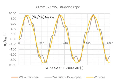
A geometrical parameter very important for the determination of the mechanical response of the wire and the rope is the first component of the tangent vector. As a matter of fact, it represents the projection of the wire local direction along the rope axis. According to equation (III.5.1) the single helix shows a constant trend. It is a consequence of the geometrical definition of this peculiar curve described in III.1. On the other hand, the double helix has a periodical trend as it can be clearly recognized in (IV.5.1).

Fig 1.17 Wire Tangent Vector First Component

-6 -4 -2 0 2 4 6 -6 -4 -2 0 2 4 6 C O M PO N EN TS x3 [m m ] COMPONENT x2 [mm] W21 outer W20 core 0.82 0.88 0.94 1.00 0 20 40 60 80 100 TA NG EN T VE C TO R FI RS T C O M PO N EN T t1 [-] ROPE AXIS x1[mm] W21 outer W20 core

36

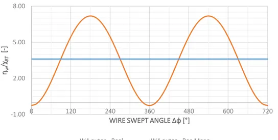
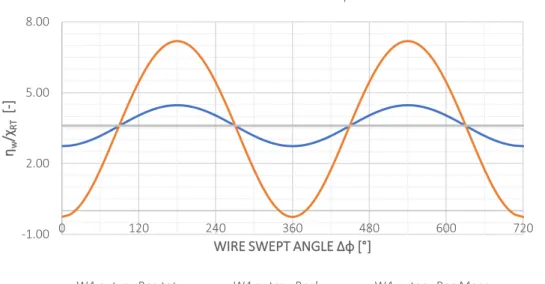
1.4. ARCH LENGH OF THE WIRE

The comparison between the two different approaches for the computation of the arch length of the double helix, already introduced with the relations (IV.5.2), is shown below.

Fig 1.18 Wire Arch Length

The following table show the errors in percentage for the maximum, minimum and mean values of the real geometry compared with the developed view.

Table 1.2 Arch Length

W20 W21 dev W21 real error

max 1.13 5.24%

min 1.06 -1.31%

mean 1.06 1.07 1.09 1.97%

The result is very important for two aspects. Firstly, the mean value of the real arch length is the geometrical parameter directly related to the global response of the rope in terms of strain, since the integration of the oscillations about the wire will filter out only the mean. Conversely, the maximum and minimum influence the local response of the single wire in terms of stresses. Hence, the choice of one of the two geometrical representations influences the system response.

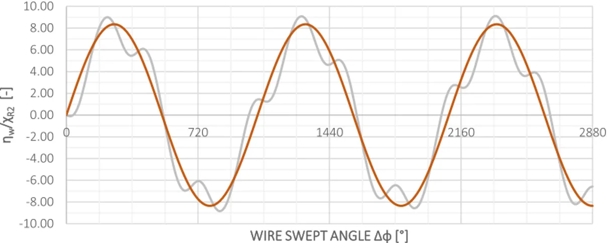
1.5. CURVATURE AND TORSION

The results are reported as functions of the swept angle of the double helix. In this manner, the dependence on the initial swept angle is lost. Moreover, it is worth to remember that due to the differential relation of the developed view (IV.3.2), the aforesaid angle is linearly related to the rope longitudinal axis, hence it is the same to talk in terms of one or the other because the difference is only a scale factor between them.

∆𝜑(𝑥1) = 𝜑(𝑥1) − 𝜑0= tan 𝛼𝐼𝐼 𝑅𝐼𝐼 cos 𝛼𝐼 𝑥1 1.04 1.06 1.08 1.10 1.12 1.14 0 20 40 60 80 100 d s/d x1 [-] ROPE AXIS x₁[mm]