ALMA MATER STUDIORUM
UNIVERSITA' DI BOLOGNA
SCUOLA DI SCIENZE
Corso di laurea magistrale in Biologia Marina
Gene expression responses to acute and
chronic heat stress in the common
reef-building coral Pocillopora verrucosa
Tesi di laurea in Adattamenti degli animali all’ambiente marino
Relatore
Presentata da
Prof. Elena Fabbri
Davide Poli
Correlatore
Dott. Silvia Franzellitti
Index
1 INTRODUCTION ... 1
1.1 THE GREENHOUSE EFFECT AND THE GLOBAL WARMING ... 4
1.2 CLIMATE CHANGE AND OCEAN ECOSYSTEM ... 6
1.2.1 The ocean in the earth system ... 7
1.3 CLIMATE CHANGE ON CORAL REEFS:BLEACHING EVENT ... 9
1.4 GEOGRAPHIC REGION DESCRIPTION –CORAL TRIANGLE ... 13
1.5 POCILLOPORA VERRUCOSA ... 17
1.6 GENES DESCRIPTION ... 20
1.6.1 NADH dehydrogenase (NDH: Bay, L. K., 2013) ... 22
1.6.2 ATP synthase ... 23
1.6.3 HSP70 ... 25
2 AIM OF THE PROJECT ... 27
3 MATERIALS AND METHODS ... 27
3.1 SAMPLES COLLECTION ... 28
3.2 ANIMAL HOLDING CONDITIONS AND EXPERIMENTAL SETUP ... 30
3.3 RNAEXTRACTION AND CDNA PREPARATION ... 33
3.4 REAL TIME PCR ASSAYS ... 33
3.5 STATISTICAL ANALYSES ... 37
4 RESULTS ... 39
4.1 TRANSCRIPTIONAL PROFILES UNDER FIELD CONDITIONS ... 41
4.2 EFFECTS OF ACCLIMATIAZATION TO THE LABORATORY CONDITIONS ... 44
4.3 TRANSCRIPTIONAL RESPONSES FOLLOWING P. VERRUCOSA EXPOSURE TO SEAWATER TEMPERATURE INCREASE UNDER LABORATORY CONDITIONS ... 47
4.4 CLUSTERING ANALYSIS ... 51
5 DISCUSSION AND CONCLUSION ... 53
5.1 CONCLUSION ... 57
1 INTRODUCTION
Summary
The Greenhouse effect and the Global Warming
The greenhouse effect is a climatic and atmospheric effect that shows the capacity of a planet to keep part of the solar energy within the atmosphere; but how it works?
Climate change and ocean ecosystem
All the elements of the earth, land, oceans, and atmosphere, appear not only connected but interdependent. The Global Warming is rising the global average surface temperatures. Many measurement have shown upward trends in all regions, and have shown that rates of change are now greater than 2°C per century in many tropical seas.
Climate change on coral reefs: Bleaching event
What happen in places where the organism can’t escape from the warming? Elevated sea temperatures as small as 1°C above long-term summer averages lead the loss of coral algal symbiont, and coral’s dead.
Geographic Region description – Coral Triangle
The CT was delineated on the basis that it is an area that contains a high proportion of the species diversity of the Indo-Pacific and that this diversity occurs in an area small enough to permit meaningful conservation.
Pocillopora verrucosa
It have true verrucae which are evenly sized and spaced. This specie occurs between the surface to 40 m deep.
Genes description
The genes useful for this study were chosen from two different kind of possible genes: two basic life genes and one that intervene during the stress event to restore the constitutive cellular environment.
INTRODUZION
Coral reefs are essential spawning, nursery, breeding, and feeding grounds for numerous organisms. In terms of biodiversity, the variety of species living on a coral reef is greater than in any other shallow-water marine ecosystems and is one of the most diverse on the planet, yet coral reefs cover less than one tenth of one percent of the ocean floor (Spalding, MD, Ravilious D, and Green EP 2001). During the last decade this habitats are threatened with worldwide decline from multiple factors, chief among them climate change (Hoegh-Guldberg O. et al. 2007; Hughes TP et al. 2003). The ability of corals to cope with this change, such as increased temperature, relies on the physiological mechanisms of acclimatization and long-term genetic adaptation. There is sample evidence that corals can be tolerant of and even thrive in temperature extremes (Coles SL, Brown BE 2003). During mass coral bleaching events, survival of scattered coral colonies suggests that some groups of corals may possess inherent physiological tolerance to environmental stress (Marshall PA, Baird AH 2000; West JM, Salm RV 2003). In addition, some high-temperature environments naturally retain healthy, growing coral populations (Coles S 1997; Oliver TA, Palumbi SR 2011), and these corals can show elevated bleaching tolerances (e.g. refs. Jokiel PL, Coles SL 1990; Oliver TA, Palumbi SR 2011). But what are the mechanisms that result in differences in thermal tolerance and physiological response? Are they due to genotypic adaptation where selection drives differences in susceptibility over evolutionary times scales or rather are they due to phenotypic acclimatization where organisms respond to extremes using their existing genomic repertoire within the lifetime of an individual? (Weis VM 2010). Under simulated bleaching stress, sensitive and resilient corals change expression of hundreds of genes, but the resilient corals had higher expression under control conditions across many genes. These “frontloaded” transcripts were less up-regulated in resilient corals during heat stress and included thermal tolerance genes such as heat shock proteins and antioxidant enzymes, as well as a broad array of genes involved in apoptosis regulation, tumor suppression, innate immune response, and cell adhesion (Barshis DJ et al. 2013). Thus represent an essential source of information about mechanisms underlying observed differences in coral physiological resilience. In this study we intend to deepen into the fundamental cellular processes responsible for enhanced stress tolerances that may enable some organisms to better persist into the future in an era of global climate change.
1.1 The Greenhouse effect and the Global Warming
The greenhouse effect is a climatic and atmospheric effect that shows the capacity of a planet to keep part of the solar energy within the atmosphere. It is part of the complex mechanisms for the thermic regulation of the planet and it operate through the presence in atmosphere of some gases called “Greenhouse gases” (Hansen J - Earth's Energy
Imbalance). The atmosphere began about 4.5 BY ago, as a mixture of water vapor,
hydrogen, hydrogen chloride, carbon monoxide, carbon dioxide and nitrogen (Gray, 2002). Through interaction with surface rocks and living organisms, it gradually reached its present composition, some 280 million years (MY) ago and has remained, more or less, unchanged (Khandekar 2005). During the past 4.5 BY to 280 MY, the most important transformation was the conversion of much of the carbon dioxide (CO₂) into oxygen by abundant plant life, particularly during the carboniferous period, when most of our coal and
oil deposits were formed (Gray, 2002). The gases nitrogen and oxygen that make up the
bulk of the atmosphere neither absorb nor emit thermal radiation. If they were the only atmospheric constituents there would be no clouds and no greenhouse effect (Houghton 2005). The atmosphere is composed either of water vapor, carbon dioxide, ozone, methane and nitrous oxide: greenhouse gases. Sun’s radiation is mostly in short wavelengths and passes through the atmosphere without much absorption, except the ultraviolet part of the solar radiation which is absorbed by ozone in the stratosphere (Figure n.1.1). Solar radiation heats the earth and the oceans and they in turn emit radiation back to space in longer wavelengths, hence known as longwave radiation. The greenhouse gases in the atmosphere, including water vapor and CO₂ absorb this longwave radiation from the earth (and oceans) and in this process, maintain an annual global surface temperature of about 14 °C to 15 °C (Khandekar 2005). Without this effect the average Earth’s surface temperature would be
Figure n. 1.1 – Global mean energy budget under present-day climate conditions. Numbers state magnitudes of the individual energy fluxes in Wm⁻², adjusted within their uncertainty ranges to close the
energy budgets. Numbers in parentheses attached to the energy fluxes cover the range of values in line with observational constraints. (TOA: radiation budget at the top of the atmosphere) (Wild et al., 2013)
The effect was first recognized by the French scientist Jean-Baptiste Fourier in 1827 (Mudge F.B. 1997). This climate system can respond to changes in external forcing: physical factors external to the climate system that force a net increase (positive forcing)
or net decrease (negative forcing) of heat in the climate system as a whole (Hansen, Sato
et al. 2005). Examples of external forcing include changes in atmospheric composition
(e.g., increased concentrations of greenhouse gases), solar luminosity, volcanic eruptions, and variations in Earth's orbit around the Sun. However this response capacity can be overcome when the external forces had a synergic effect in a long term period of time
(Gray, 2002). A British scientist, John Tyndall around 1860 measured the absorption of
infrared radiation by carbon dioxide and water vapor and suggested that a cause of the ice ages might be a decrease in the greenhouse effect of carbon dioxide. It was a Swedish chemist, Svante Arrhenius in 1896 who first calculated the effect of increasing concentrations of greenhouse gases; he estimated that doubling the concentration of carbon dioxide would increase the global average temperature by 5–6°C (Houghton J. 2005).
1.2 Climate change and ocean ecosystem
A rise in global average surface temperatures is the best-known indicator of climate change. Although each year and even decade is not always warmer than the last, global surface
temperatures have warmed substantially since 1900 (Hartmann D.L. et al. 2013).Warming
land temperatures correspond closely with the observed warming trend over the oceans. Warming oceanic air temperatures, measured from aboard ships, and temperatures of the sea surface itself also coincide, as borne out by many independent analyses (Hartmann D.L. et al. 2013). A global perception started to emerge, recognizing that the earth was a single, interconnected unit, within which the biosphere is an active and essential component. All the elements of the earth, land, oceans, and atmosphere, appear not only connected but interdependent. Surely an impact on one of these components must reflect on the others and on the whole. However, the extent to which the earth behaves as a single, interlinked, self-regulated system was not put into focus until scientists reconstructed the chemical history of the earth’s atmosphere from 420,000-year-old Antarctica ice cores (the Vostok record; Petit et al. 1999), and more recently from the 650,000-year-old cores from European Project for Ice Coring in Antarctica (EPICA) (Siegenthaler et al. 2005). These data indicated that the CO₂ levels in the atmosphere had been constrained between 180 and 290 ppm by volume for over 500,000 years, with minima and maxima corresponding to the glacial and interglacial periods, respectively. Equivalent cycles from atmospheric temperature proxies demonstrated a strong coupling between climate and the carbon cycle as well as the stability of this coupling over the recorded time. For some time scientists have suspected that the glacial/interglacial cycles that the earth has experienced every 100 kyr (Siegenthaler et al. 2005) are caused by smooth changes in the eccentricity of the earth’s orbit. However, these changes are too smooth to generate such sharp, non-linear responses in the chemical composition of the atmosphere, unless these are strongly modulated by biological, chemical, and physical feedbacks (Barange M. et al. 2010). Furthermore we have to consider that the earth system responds to the physical forces in complex ways, often non-linearly. These responses involve interactions between land, atmosphere, water, ice, biosphere, societies, technologies, and economies.
1.2.1 The ocean in the earth system
The ocean is one of the major components of the earth system, providing 99% of the available living space on the planet. Water is essential to our existence, having secured life from the time of the primeval soup. It has been estimated that 80% of all life on earth depends on healthy oceans and coasts and more than a third of the world’s population lives in coastal areas and small islands, even though they amount to less than 4% of the earth’s land. The ocean’s heat capacity is about 1,000 times larger than that of the atmosphere, and the oceans net heat uptake since 1960 has been around 20 times greater than that of the atmosphere (Bindoff et al . 2007). Long-term records, starting at various points in the 20th century, additional observations, including balloon-borne measurements and satellite measurements, and reanalysis products allow analyses of indicators such as atmospheric composition, radiation budgets, hydrological cycle changes, extreme event characteriza-tions and circulation indices show how global trends in Greenhouse Gases (GHGs) are indicative of the imbalance between sources and sinks in GHGs budgets, and play an important role in emissions verification on a global scale (Wielicki et al., 1996, Kopp and Lawrence, 2005) . IPCC (2007) has demonstrated that increasing atmospheric burdens of well-mixed G in a 9% increase in their RF from 1998 to 2005. These trends resulted in a 7.5% increase in RF from GHGs from 2005 to 2011, with carbon dioxide (CO₂) contributing 80%. Of note is an increase in the average growth rate of atmospheric methane (CH₄) from ~0.5 ppb yr⁻¹ during 1999–2006 to ~6 ppb yr⁻¹ from 2007 through 2011
(Hartmann D.L. et al. 2013). ‘Recent’ warming (since the 1950s) is strongly evident at all
latitudes in SST over each ocean. Prominent spatio-temporal structures including the ENSO and decadal variability patterns in the Pacific Ocean and a hemispheric asymmetry in the Atlantic Ocean were highlighted as contributors to the regional differences in surface warming rates, which in turn affect atmospheric circulation. There are direct evidence to conclude that the world oceans have warmed substantially (Figure n.1.2) over the last half century, and that the warming accounts for over 80% of the changes in the
energy content of the earth’s climate system during this period (Bindoff et al. 2007; Domingues et al. 2008). A large-scale coherent trend of salinity and observed changes in precipitation are also observed. More water is transported in the atmosphere from low latitudes to high latitudes producing a global regime shifts, as well expected poleward range shift and freshening in sub- polar latitudes and a salinification of shallower parts of the tropical and subtropical oceans (Barange M. et al. 2010). Increases of 1-2°C in sea temperature are expected by 2100 in
Figure n.1.2: Observation-based estimates of annual global mean upper (0 to 700 m) ocean heat content in ZJ (1 ZJ = 1021 Joules) updated from (see legend): Levitus et al. (2012), Ishii and Kimoto (2009), Domingues et al. (2008), Palmer et al. (2007) and Smith and Murphy (2007). Uncertainties are shaded and plotted as published (at the one standard error level, except one standard deviation for Levitus, with no uncertainties provided for Smith).(Rhein, M. 2013)
response to enhanced concentrations of atmospheric greenhouse gases (Bijlsma et al. 1995). Sea temperatures over the past 20 years, extensively measured and cross-compared by instruments on satellites, ships and buoys, have shown upward trends in all regions, and have shown that rates of change are now greater than 2°C per century in many tropical seas
(O. Hoegh-Guldberg 1999). This global trend, however, has not been homogeneous or
linear. Significant decadal variations have been observed in the sea surface temperature (SST) time series, and there are large regions where the oceans have been cooling (Bindoff
et al. 2007; Harrison and Carson 2007).Although the oceans are interconnected, there are
specific modes of response to forcing that show important differences as well (Barange M.
et al. 2010, Drinkwater K.F. 2003). Alternating short-term and long-term event (e.g. El
Niño –Southern Oscillation (ENSO) and Pacific Decadal Oscillation (PDO) in the Pacific
Ocean) provides ways of moving heat from the tropical ocean to higher latitudes and out of the ocean into the atmosphere (Trenberth et al. 2002). The dynamic nature of the different oceans, exemplified by the varying heat exchange processes, is responsible for the diversity of marine environments and habitats. The properties of water generate different density layers and gradients. Tides, currents, and upwelling break this stratification and, by forcing the mixing of water layers, enhance primary production. This network of surface and deep water currents tightly connects marine ecosystems and defines its dynamics (Drinkwater K.F. 2009).
1.3 Climate change on coral reefs: Bleaching event
Decades of ecological and physiological research document that climatic variables are primary drivers of distributions and dynamics of marine plankton and fish (Hays et al.2005, Roessig et al. 2004). Globally distributed planktonic records show strong shifts of phytoplankton and zooplankton communities in concert with regional oceanic climate as changes in timing of peak biomass (deYoung et al. 2004, Hays et al. 2005, Richardson & Schoeman 2004). Some copepod communities have shifted as much as 1000 km northward (Beaugrand et al. 2002). The data show a significant increase in southern-ranged species in that geographic regions had experienced a period of significant warming in SST and decrease of northern-ranged species. Likewise the regions (e.g. United Kingdom) that experienced a significant cooling in SST have seen the shifting of the community to a northern-ranged species (Sagarin et al. 1999, Southward et al. 2005). But what happen in places where the organism can’t escape from the warming? What happen to the coral reefs? Elevated sea temperatures as small as 1°C above long-term summer averages lead the loss of coral algal symbiont , and global SST has risen an average of 0.1°–0.2°C since 1976 (Hoegh-Guldberg 1999, IPCC 2001). Coral bleaching, the paling of tissues resulting from the drastic decline in zooxanthella densities and/or the loss of photosynthetic pigments which occurs when the thermal tolerance of corals and their photosynthetic symbionts (zooxanthellae) is exceeded, is a classic stress response of corals and allied symbiotic marine animals to perturbations in environmental conditions (Glynn, 1993, Brown, 1997, Hoegh-Guldberg O. 1999).
The central feature of shallow-water coastal ecosystems, known since the middle of the last century (Odum and Odum 1955), is the predominance of symbioses between invertebrates and dinoflagellate microalgae commonly referred as "zooxanthellae". All the Reef-building corals, the heart of coral reefs, are obligate endosymbiotic with algae of the dinoflagellate genus Symbiodinium (Mieog et al. 2009). Symbiodinium is the most studied genus in this paraphyletic group and is commonly found in shallow water tropical and subtropical cnidarians. These algae are ubiquitous members of coral reef ecosystems (Rowan 1998, Taylor 1974, Trench 1993): Cnidarian species reported to contain Symbiodinium include many representatives from the class Anthozoa (including anemones, scleractinian corals, zoanthids, corallimorphs, blue corals, alcyonacean corals, and sea fans) and several
and Hydrozoa (including milleporine fire corals) (Baker A.C. 2003). Members of six of the eight Symbiodinium clades (A–D, F, G) are known to associate with scleractinian corals, the reef builder corals (Baker A.C. 2003). It is not uncommon for the same coral colony to
harbour multiple clades (reviewed by Baker A.C. 2003; Mieog et al. 2007) or types of
symbionts simultaneously. Some species also undergo seasonal change in their endosymbiont community (Chen et al. 2005). These zooxanthellae are intracellular (Trench 1979) and are found within membrane-bound vacuoles in the cells of the host. Zooxanthellae photosynthesize while residing inside their hosts, and provide energy and nutrients for the invertebrate host by translocating up to 95% of their photosynthetic production to it (Figure n.1.3a) (Muscatine 1990; Woldridge S.A and Done T.J. 2009). Zooxanthellae selectively leak amino acids, sugars, complex carbohydrates and small peptides across the host-symbiont barrier. These compounds provide the host with a supply of energy and essential compounds (Muscatine 1973; Trench 1979; Swanson and Hoegh-Guldberg 1998). Corals and their zooxanthellae form a mutualistic symbiosis, as both partners appear to derive benefit from the association. Corals receive photosynthetic products (sugars and amino acids) in return for supplying zooxanthellae with crucial plant
nutrients (ammonia and phosphate) from their waste metabolism (Trench 1979).The latter
appear to be crucial for the survival of these primary producers in a water column that is normally devoid of these essential inorganic nutrients. Dubinsky Z. and Jokiel P.L. (1994) seen that when corals exposed to various light intensities, in corals exposed with Low-Light intensity, photosynthesis alone cannot account for all of the colony respiration; therefore such colonies have to supplement zooxanthellae autotrophy with heterotrophic animal predation on zooplankton (Falkowski et al. 1984). Indeed, under low light, most corals remain with their tentacles extended continuously, showing the needing to hunt more for zooplankton to supply to all the energy request (Dubinsky Z. and Jokiel P.L. 1994). This close association of primary producer and consumer makes possible the tight nutrient recycling that is thought to explain the high productivity of coral reefs (Muscatine and Porter 1977). Reef-building corals are greatly influenced by the biological and physical factors of their environment. Temperature, salinity and light have major effects on where reef-building corals grow. Environments in which coral reefs prosper are also typified by a high degree of stability (Hoegh-Guldberg O. 1999). Sea temperatures in many tropical regions have increased by almost 1°C over the past 100 years, and are currently increasing at ~1.2°C per century. When this changes occur too rapidly the thermal tolerance of corals
and their photosynthetic symbionts (zooxanthellae) is exceeded. This causes the breakdown of the symbiosis (coral bleaching) and a significant proportion of the zooxanthellae compliment is expelled from the coral animal (Coles and Jokiel 1977, 1978; Glynn and D.Croz 1990; Lesser et al. 1990; Brown 1997).
The warm-water bleaching syndrome of the coral–algae endosymbiosis follows a sequence of algal photoinhibition, oxidative damage, and host cell membrane disruption (e.g., Gates et al. 1992, Lesser 1996, Jones et al. 1998, Warner et al. 1999). Wooldridge (2009) proposes that the onset of this sequence is linked with a disruption to the ‘‘dark’’ photosynthetic reactions of the algal endosymbionts, implicating limited availability of CO₂ substrate around the Rubisco enzyme (Figure n.1.3b). In this way, biophysical factors that cause CO₂ demand to exceed CO₂ supply within the coral’s intracellular milieu are identified as bleaching risk factors.
Figure.n 1.3 – (a) Schematic overview of the internal carbon cycling that is maintained by the coral– zooxanthellae symbiosis. (b)Schematic representation of the breakdown of the symbiosis (¼zooxanthellae expulsion), as triggered by a limitation of CO2 substrate for the ‘‘dark’’ reactions of
Figure.n1.4 – Healthy, bleached and dead organisms of the species Plerogyra sp. in Bangka island, North Sulawesi, Indonesia (Photo credit: Davide Poli 2014)
1.4 Geographic Region description – Coral Triangle
Figure.n 1.5 – Extension of the Coral Triangle. official CTI-CFF regional map (Peterson N. 2011)
“If we look at a globe or a map of the Eastern Hemisphere, we shall perceive between Asia and Australia a number of large and small islands, forming a connected group distinct from those great masses of land and having little connection with either of them. Situated upon the equator, and bathed in the tepid water of the great tropical oceans, this region enjoys a climate more uniformly hot and moist than almost any other part of the globe, and teems with natural productions which are elsewhere unknown.” So begins Alfred Russel
Wallace’s seminal book “The Malay Archipelago”, first published in 1869 (Wallace, 1869). That was the born of the biogeography and MacArthur and Wilson escorted the field into the modern age in 1963 with their theory of island biogeography (Barber PH. 2009). These as well as other authors of the time have almost completely ignored the marine reign although there were occasional attempts to map marine life, notably by the American geologist James Dana (1853), the British naturalist Edward Forbes (1856) as well as Charles Darwin himself (1859). There were a few scattered publications on the distribution of some marine taxa during the latter part of the 19th century (George 1981), but it was not until the publication of Bartholomew’s Atlas in 1911 and Ekman’s historic compendium in 1935 that marine biogeography became established as a science in its own right (Veron
marine biodiversity of varying shapes, all centered on the Indonesian/Philippines Archipelago. Some stem from biogeographic theory or geological history, others from coral and reef fish distributions. These centers have been given a variety of names: Wallacea, East Indies Triangle, Malayan Triangle, Western Pacific Diversity Triangle, Indo-Australian Archipelago, South-east Asian center of diversity, Central Indo-Pacific biodiversity hotspot, Marine East Indies, among others (Hoeksema 2007).
For various reasons it is important to know where the highest concentration of species can be found: coastal areas offer a great potential of natural resources for local human populations, especially in countries rich in marine species; for the designation of a network of Marine Protected Areas (MPAs) and for other conservation efforts; the marine tourism industry benefits from the high variety of marine life; the position and boundaries of the centre of marine diversity are relevant for evolutionary and ecological problems (Hoeksema2007). Delineation of the CT (Veron JEN et al. 2009) was established by the spatial database Coral Geographic, a major update of the original species maps of Veron JEN et al. (2000). This database contains comprehensive global species maps of zooxanthellate coral distributions in GIS format, allowing them to be interrogated to compare geographic regions or to elucidate patterns of diversity and endemism (Veron JEN. et al. 2009). This coral ecoregions so identified provide a blueprint for establishing a globally representative network of coral reef MPAs. The world’s highest diversity occurs in the CT, an area where more than 500 coral species are found in each ecoregion (Veron JEN. et al. 2011). The CT was delineated on the basis that it is an area that contains a high proportion of the species diversity of the Indo-Pacific and that this diversity occurs in an area small enough to permit meaningful conservation. With this delineation, the 16 ecoregions of the CT each host >500 reef coral species (Veron JEN. et al. 2009). The CT defined by Coral Geographic – that adopted by the six-nation Coral Triangle Initiative (CTI) – is an area of 5.5 × 10⁶ km2 of ocean territory of Indonesia, the Philippines, Malaysia (Sabah), Timor Leste, Papua New Guinea, and the Solomon Islands (Figure n.1.5) less than 1.6% of the world’s total ocean area. The CT is not a distinct biogeographic unit, but comprises portions of two biogeographic regions (Indonesian-Philippines Region, and Far Southwestern Pacific Region, Veron 1995). In total, the CT has 605 zooxanthellate coral species of which 66% are common to all ecoregions. This diversity amounts to 76% of the world’s total species complement (Figure n.1.6). Within the CT, highest richness resides in the Bird’s Head Peninsula of Indonesian Papua, which hosts 574 species.
Individual reefs there have up to 280 species haˉ¹, over four times the total zooxanthellate scleractinian species richness of the entire Atlantic Ocean (Turak and DeVantier in press). Within the Bird’s Head, The Raja Ampat Islands ecoregion has the world’s coral highest biodiversity, with 553 species (Turak and Souhoka 2003). It contains 52% of Indo-Pacific reef fishes (37% of reef fishes of the world) (Allen 2007). Other major faunal groups, notably molluscs (Wells 2002) and crustaceans (Grave 2001), have very high numbers of undescribed or cryptic species and thus are relatively little-known at species level (Meyer et al. 2005). Even azooxanthellate corals, which have none of the physiological restrictions of zooxanthellate species, have a centre of global diversity within the CT (Cairns 2007).
Figure n.1.6 - Global biodiversity of zooxanthellate corals. Colours indicate total species richness of the world’s 141 coral biogeographic ‘ecoregions’ (From the spatial database Coral Geographic, Veron JEN.
et al. 2000)
So much interest from so many points of view begs the question: why does the CT exist? There are several interacting factors operating over different temporal and spatial scales: geological history; larval dispersal and genetic mixing; Biogeographic patterns; Evolutionary processes (Veron JEN. et al. 2009). The diversity of the CT has no single explanation. Plate tectonics created the biogeographic template, one of complex island coastlines and extreme habitat heterogeneity. Patterns of dispersion, mediated by ocean currents, formed sequences of attenuation away from the equator leaving the CT with the region’s highest biodiversity. Many environmental parameters, especially ocean currents and temperature, underpin this pattern. Evolutionary patterns, the genetic outcomes of environmental drivers, show why the CT is a centre of biodiversity (Veron JEN. et al. 2009). Whatever the drivers of diversity that created the CT, it is the future that matters as far as conservation is concerned. Anthropogenic increase in tropical ocean temperature has been less than 0.8°C to date but could be as much as 2–3°C this century (IPCC 2007a, b),
threat. In a business-as-usual regime of anthropogenic carbon dioxide increase, calcification of equatorial corals will be marginal by the year 2030 (Guinotte et al. 2003). From a conservation perspective, all corals are threatened by the dual process of mass bleaching and ocean acidification. Furthermore, approximately 225 million people live within the CT, of which 95% live adjacent to the 131,254 km of coast. This population is largely dependent on the productivity of coral reefs and adjacent waters and a larger population is dependent on protein from these sources. There are no estimations of the value of the reefs of the CT; however, as Indonesia’s reefs were valued at $1.6 billion annually in 2002 (Burke et al. 2002), the current value of the CT is at least $2.3 billion annually. Although correlations between ecological and economic impacts on reefs stemming from environmental decline cannot be estimated with certainty, it has been estimated that Indo-Pacific reefs are declining at >2% per year (Bruno and Selig 2007 and Burke et al. 2002) and this is becoming increasingly difficult to reverse (Hoegh-Guldberg et al. 2009).
1.5 Pocillopora verrucosa
Figure n.1.7 – Pocillopora verrucosa (Photo credit: Davide Poli 2014) Taxonomy
Kingdom Phylum Class Order Family
ANIMALIA CNIDARIA ANTHOZOA SCLERACTINIA POCILLOPORIDAE
Specific Name
Pocillopora verrucosa (Ellis and Solander 1786)
Previous name
Madrepora verrucosa
(Ellis & Solander, 1786 - original combination, basionym)
Pocillopora danae (Verrill, 1864 ) Pocillopora hemprichi (Ehrenberg, 1834 )
Common name Rasp Coral Red List Category Not Evalueted Data Deficient Least Concern Near
Threatened Vulnerable Endangered
Critically Endangered Extinct in the Wild Extinct Least Concern
Distribution This species is common
Pocillopora verrucosa have broad, club shaped or more flattened branches (Figure n.1.7).
It have true verrucae which are evenly sized and spaced. This species occurs between the surface to 40 m deep. On fore reef slopes of moderate but not extreme exposure, it is extremely common, and helps to define clear coral communities in many sites. It is not well tolerant to sedimentation, so is much less abundant in lagoon areas (Sheppard, 1998). Colonies are composed of uniform upright branches clearly distinct from the verrucae, but the latter are irregular in size. Colonies usually form hemispheres and grow in isolation. The stout branches radiate from a central holdfast and tend to be clubbed at their tips. Large verrucae are up to 6 mm high, and corallites 1 mm across. They have permanently coloured red-brown stalks. This colour can varies from pale lime-green or pink to dark brown or bluish-brown (Veron JEN. et al. 2000).
Ecology and Distribution:
Figure. n. 1.8 – Geographic distribution of Pocillopora verrucosa (Hoeksema B.W. et al. 2014)
Pocilloporid corals usually occurs in shallow reef environments (1-15m depth) but is been found till 54m depth (Reyes-Bonilla et al. 2005). This species lives in exposed reef fronts as in to protected fringing reefs in coral communities on rocky substrata. Pocilloporid, including P. verrucosa, it is amongst the strongest coral competitors (Glynn 2001) and represent one of the principal framework builders of many reefs (Glynn 2001). This species has a widespread distribution (Figure n.1.8) within the Indo-West Pacific and Eastern Tropical Pacific regions. In the Indo-West Pacific, this species is found in the Red Sea and the Gulf of Aden, the Southwest and Northwest Indian Ocean and the Arabian/Iranian Gulf, the Central Indian Ocean, the Central Indo-Pacific, Tropical Australia, Southern Japan and
the South China Sea, the Oceanic West Pacific, the central Pacific, Hawaiian Islands and Johnston Atoll, and the Far Eastern Pacific. In the Eastern Tropical Pacific, this species is found in Mexico: Baja California Sur, Nayarit, Jalisco, Colima, Michoacán, Guerrero and Oaxaca; Costa Rica: mainland Costa Rica including Cocos Island; Panama; Colombia: mainland Colombia including Malpelo Island; Ecuador: mainland Ecuador (Hoeksema B.W. et al. 2014).
Threats
The major threat is global climate change, in particular, temperature extremes leading to bleaching and increased susceptibility to disease, increased severity of ENSO events and storms, and ocean acidification. There are evidence that overall coral reef habitat has declined, and this is used as a proxy for population decline for this species. This species is more resilient to some of the threats faced by corals and therefore population decline is estimated using the percentage of destroyed reefs only (Wilkinson 2004). As reported by Glynn et al. (1988) Pocilloporid species as well as other major reef building corals catastrophically declined after 1983. This situation is exasperated, in the affected region, during the ENSO event (Glynn 2000). In addition to this threat there is the overfishing that is probably responsible for some ecological imbalance on coral reefs that could prolong recovery from other disturbances.
In addition “This species is targeted for the aquarium trade. Indonesia is the largest
exporter with an annual quota of 5,600 live pieces in 2005” (Hoeksema B.W. et al. 2014).
Coral disease are emerged as a serious threat to coral population worldwide. The increasing number of disease and population affected is related to the deterioration of the quality of the water and to the increasing of the sea surface temperature (Willis et al. 2007).
Localized threats to corals include invasive species; changes in native species dynamics; fisheries; dynamite and chemical fishing; human development; domestic, agricultural and industrial pollution; human recreation and tourism activities and sedimentation.
Pocillopora species are preyed on by some different type of consumers including species
that scrape skeletal surface (Trizopagurus, etc), species that bite off colony branch-tips (Scaridae, etc.), Species that abrade tissues and skeleton (Eucidaris galapagensis), Species
that remove tissues but leave the skeleton intact (Stegastes acapulcoensis, Acanthaster
1.6 Genes description
The genes useful for this study were chosen from two different kind of possible genes. The first type is the basic life genes. It includes all those fundamental genes needed for the normal cellular metabolism. From this pool, ATP Synthase’s and NADH Dehydrogenase’s genes were chosen. The second genes type is that one that intervene during the stress event to restore the constitutive cellular environment.
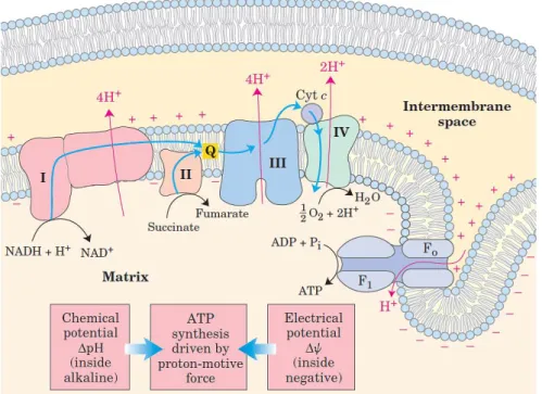
The first two genes encode for two fundamental protein complexes for the process of ATP production: the Oxidative Phosphorylation (Figure n.1.9). This process represents the final stage of the energetic metabolism of the aerobic organisms. All the enzymatic step of the oxidative degradation of the carbohydrates, of the fat acids and of the aminoacids within the aerobic cells converge to the final step of the cellular respiration (Nelson D.L. and Cox M.M.). In this stage the oxidative energy is used for the production of ATP. In Eukaryotic cells the oxidative phosphorylation runs in the mitochondria where through the electron
provided by NADH and FADH₂the oxygen is reduced to water. All these processes are
based on the Chemiosmotic Theory (Nelson D.L. and Cox M.M.), a Peter Mitchell hypothesis where the energetic transduction is made throw the creation of trans-membrane gradient. The mitochondria have two membranes. The outer membrane is easily permeable from the ion moving throw a transmembrane channels. These channels are part of a family of integral membrane proteins called porins. The inner membrane is almost completely impermeable to all the small molecules and ions, including the protons (H⁺). The only chemical species that can go through it are the ones that have a specific transmembrane transporter. In this structure are included the component of the respiration chain and the ATP synthesis enzymatic complex. ADP and Pᵢ are transported to the inner mitochondria and at the same time the ATP is transported out of the organelle. The electrons carriers of the respiratory chain are organized in membrane-embedded supramolecular complex. Each of this complex represents part of the respiratory chain and has the capacity to catalyze the electrons transfer thorugh the chain (Nelson D.L. and Cox M.M.). The complex I and II transfer the electrons to the ubiquinone from two different donors: NADH (complex I) and succinate (complex II). The Complex III transport the electrons from the ubiquinone to the cytochrome c and the Complex IV close the sequence carrying the electrons to the oxygen (Djafarzadeh R., 2000).
1.6.1 NADH dehydrogenase (NDH: Bay, L. K., 2013)
The oxidative phosphorylation starts in the respiratory chain with the electrons input. The majority of these electrons are from the action of dehydrogenase enzymes working in the catabolic processes. These electrons are transported to the universal acceptor: the nicotinamide nucleotides (NAD⁺ or NADP⁺) or flavin nucleotides (FMN or FAD) (Fearnley I. M. & Walker J. E. 1992). The complex I is a large dimension enzyme with more than 42 different polypeptide chains including a FMN-containing flavoprotein and at least six iron-sulfur centers. The oxidized flavin nucleotide (FMN) can accept either one electron or two (Djafarzadeh R., 2000). Electron transfer occurs because the flavoprotein has a higher reduction potential than the compound oxidized. In the iron-sulfur center the iron is associated with inorganic sulfur atoms or with the sulfur atoms of Cys residues in the protein, or both. All iron-sulfur proteins are involved in redox reactions with one-electron transfer in which one iron atom of the iron-sulfur cluster is oxidized or reduced. The Complex I it is a L-shaped protein with one arm of the L in the membrane and the other extending into the matrix (Djafarzadeh R., 2000). This NAD⁺-linked dehydrogenases remove two Hydrogen atoms from their substrates. One of these is transferred as a Hydride ion (:H⁻) to the NAD⁺; the other ion is released to the medium as a H⁺.
NADH + H⁺ + CoQ + 4H⁺in → NAD⁺ + CoQH₂+ 4H⁺out (Nelson D.L. and Cox M.M.)
Simultaneously it catalyzes the endergonic transfer of four protons from the matrix to the intermembrane space (Figure n.1.10).
The Complex I is a proton pump driven by the energy of electron transfer. The reaction catalyzed is vectorial because it moves the protons in one specific direction from one location (the matrix, which becomes negatively charged with the departure of protons) to another (the intermembrane space, which becomes positively charged).
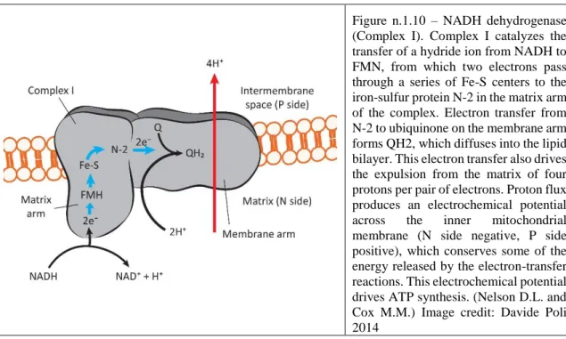
Figure n.1.10 – NADH dehydrogenase (Complex I). Complex I catalyzes the transfer of a hydride ion from NADH to FMN, from which two electrons pass through a series of Fe-S centers to the iron-sulfur protein N-2 in the matrix arm of the complex. Electron transfer from N-2 to ubiquinone on the membrane arm forms QH2, which diffuses into the lipid bilayer. This electron transfer also drives the expulsion from the matrix of four protons per pair of electrons. Proton flux produces an electrochemical potential across the inner mitochondrial membrane (N side negative, P side positive), which conserves some of the energy released by the electron-transfer reactions. This electrochemical potential drives ATP synthesis. (Nelson D.L. and Cox M.M.) Image credit: Davide Poli 2014
1.6.2 ATP synthase
The F-type ATPase active transporters play a central role in energy-conserving reactions in mitochondria, bacteria, and chloroplasts. The F-type ATPases catalyze the uphill transmembrane passage of protons driven by ATP hydrolysis (Boyer P.D. 1997). The mitochondrial ATP-synthase is one of these ATPase and it catalyzes the formation of ATP from ADP and Pᵢ as starting substrates, coupled with the proton flux from the P side to the
N side of the membrane. The ATP synthase, also known as Complex V, has two distinct
components: F₁, a peripheral membrane protein, and Fₒ (“o” denoting oligomycin-sensitive), which is integral to the membrane. In the laboratory is been demonstrated that the F₁ subunit can catalyze electron transfer from NADH to O₂ even if separated from the Fₒ subunit but cannot produce a proton gradient: Fₒ has a proton pore through which protons leak as fast as they are pumped by electron transfer, and without a proton gradient the F₁-depleted vesicles cannot make ATP (Nelson D.L. and Cox M.M.). Every F₁ complex has nine subunits of five different types, with the composition α₃β₃γδε (Figure n.1.11).
Figure n.1.11 - Mechanism of ATP production by ATP synthase. (Murray R.K. 2009)
The F1 portion is a flattened sphere, 8 nm high and 10 nm across, consisting of alternating α and β subunits arranged like the sections of an orange. The amino acid sequences of the three β subunits are identical but they have different conformation. These conformational differences among the β subunit extend to differences in their ATP/ADP-binding sites. One of the three subunits binds ATP, one ADP and one is empty because it is bound with the γ subunit and it is called β-empty. The other two are called respectively β-ATP and β-ADP (Capaldi R.A. and Aggeler R. 2002). On the basis of kinetic studies, Paul Boyer proposed the rotational catalysis mechanism in which the three β active sites of the F₁ subunit take turns catalyzing ATP synthesis (Boyer P.D. 1997). The Fₒ complex making up the proton pore is composed of three subunits, a, b, and c, in the proportion Ab₂c₁₀ˍ₁₂. Subunit c is a small very hydrophobic polypeptide, consisting almost entirely of two transmembrane helices, with a small loop extending from the matrix side of the membrane. The flow of electrons through Complexes I, III, and IV results in pumping of protons across the inner mitochondrial membrane, making the matrix alkaline relative to the intermembrane space (Senior A.E. et al. 2002). This proton gradient provides the energy (in the form of the proton-motive force) for ATP synthesis from ADP and Pᵢ by ATP synthase (FₒF₁ complex) in the inner membrane. ATP synthase carries out “rotational catalysis,” in which the flow
of protons through Fₒ causes each of three nucleotide-binding sites in F₁ to cycle from (ADP + Pi)–bound to ATP-bound to empty conformations (Capaldi R.A. and Aggeler R. 2002). ATP formation on the enzyme requires little energy; the role of the proton-motive force is to push ATP from its binding site on the synthase.
1.6.3 HSP70
With the HSP70 term (Heat Shock Proteins 70 kilodaltons) is indicated a protein family both important for the normal proteins folding processes and involved in the heat shock response assisting the stress-denatured proteins. This family was discovered accidentally in the 60s during a study on Drosophila often called "fruit flies". Involuntarily one sample of this species was exposed to a higher temperature of the normal study case and during the microscopic observation of the chromosomes was noticed an elevate transcription of these unknown proteins (Yoshimune K et al., 2002). This unpredicted response has been called “Heat Shock Response” and these proteins have been called "Heat Shock Proteins" (HSPs). As central components of the cellular protein surveillance network these ATP-dependent chaperones are involved in a large variety of protein-folding processes and they are highly conserved in evolution (Mayer MP. 2013). HSP70s demonstrate a 60–78% base identity among eukaryotic cells and a 40–60% identity between eukaryotic HSP-70 and Escherichia coli DnaK (Caplan et al., 1993). These chaperones are central players in protein folding and proteostasis control and they regulate a large number of protein folding such as de novo folding of polypeptides, refolding of misfolded proteins and the regulation of stability and activity of certain natively folded proteins that were regulated in their activity, stability, and/or oligomeric state (Mayer MP. and Bukau B. 2005). This Chaperone machine is composed of an N-terminal 40-kDa ATP-binding domain and a C-terminal 30-kDa substrate-binding domain (SBD). The wide applicability of HSP70 is because they don’t enclose entirely their substrate but they bind just a short part of it in the SBD domain. In this way their application is not limited by the dimension of the substrate. In this way, the
HSP group is very versatile assisting in a large amount of protein-folding processes(Richter
et al. 2010) from de novo polypeptide folding to translocation of proteins across the membrane. This features, linked to the fact that genes encoding HSP70 lack introns allowing a more rapid response to stress (Boutet et al. 2003), reflect the frequency of up-regulation and concentration during stress situation (Lewis et al. 1999). The interaction
domain (NBD) (Figure n.1.12) (Mayer M.P. 2010). The ATP-dependent reactions are regulated by co-chaperones of the HSP40 (also known as DnaJ) (Hartl F.U et al. 2011). This because Hsp70s do not work alone but with a team of co-chaperones because the intrinsic ATP hydrolysis rates of Hsp70s are generally low, with one molecule of ATP being hydrolyzed per Hsp70 molecule per 20–30 min at 30°C (e.g., Escherichia coli DnaK, human Hsp70)(Mayer M.P. Et al. 2000; Gässler C.S. et al. 2001 Mayer M.P. 2013). In the ATP-bound state, association of peptides to the SBD and peptide dissociation from the SBD occurs at high rates, but affinity for polypeptides is low (Mayer M.P. 2010; Mayer M.P. 2013). In the ADP-bound and nucleotide-free states, after ATP hydrolysis by the NBD, peptide association and dissociation rates are decreased by several orders of magnitude, leading to an increase in affinity for substrate peptides and a low exchange rates (Schmid D. et al. 1994).
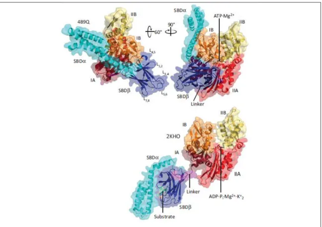
Figure n.1.12 - Cartoon and surface representation of the ATP-bound open conformation of Escherichia coli DnaK (PDB code 4B9Q), in two orientations as indicated, and of the ADP-bound closed conformation of E. coli DnaK (PDB code 2KHO; lower panel); NBD is in the same orientation as upper right panel. Subdomains of the NBD are shown in dark red (IA), red (IIA), orange (IB), and yellow (IIB); the linker is in magenta, SBDb is dark blue and SBDa is cyan, and the substrate is green. The loops of the SBDb are designated as L1,2 to L7,8 (Bertelsen, E.B. et al. 2009)
2 AIM OF THE PROJECT
AIM OF THE PROJECT
The aim of this study was to increase the understanding of the basic cellular processes responsible for enhanced stress tolerance that may enable organisms to tolerate climate change. In particular, for reef-building corals dramatic declines in abundance are expected to worsen as anthropogenic climate change intensifies. Recent evidence has called into question whether corals have the capacity to acclimatize or adapt to global climate change and some groups of corals may possess inherent physiological tolerance to environmental stress. Such a physiological tolerance would enable specific corals to cope with future climate change. Different corals differ substantially in physiological resilience to environmental stress, but the molecular mechanisms behind enhanced coral resilience remain unclear.
At the molecular level, enhanced thermotolerance in other marine organisms, including intertidal limpets, mussels, and sea cucumbers, has been related to higher basal expression of heat shock proteins, mainly HSP70, together with the ability to develop an inducible HSP response, activation of some enzymes, cytoskeletal reorganization, cell signaling and transcriptional modulation. Recently, a wide transcriptomic approach was carried out in Acropora hyacinthus addressing the genomic basis for coral resilience. The present work focused on three specific gene products (namely ATP synthase; NADH dehydrogenase and Heat Shock Protein 70kDa ) and mRNA expression patterns underlying differences in thermal resilience were investigated in specimen of the common reef-building coral Pocillopora verrucosa collected at different locations in Bangka Island waters (North Sulawesi; Indonesia). Moreover, to identify potential mechanisms behind physiological resilience a thermal stress experiment using 174 colonies of P. verrucosa was performed under controlled conditions.
3 MATERIALS AND METHODS
Summary
Samples Collection
Each site was been characterized in order to understand the percentage cover of the chosen species and the principal categories of organism.
Animal holding conditions and experimental setup
Experimental design, methods and equipment to perform the experiment.
mRNA Extraction, and cDNA preparation
Techniques utilized to prepare the mNA for the Gene Expression Analysis.
Real Time PCR assays
Instrument and methods
Statistical Analysis
3.1 Samples Collection
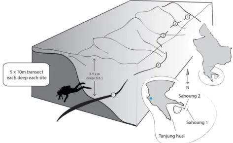
Figure n. 3.2 a and b – Geographic location of the three sampling sites Sahoung 1 (SA1), Sahoung 2 (SA2), and Tanjung Husi (TA) located in the South-Est side of the island. Relative distance between SA1 and SA2: 210m; Relative distance between SA1 and TA: 1350m; Relative distance between SA2 and TA: 1370m. (Base Map: Google earth).
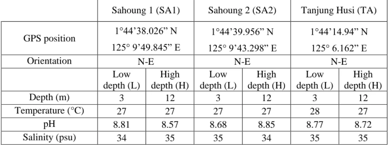
Experiments were performed at the CoralEye Reef Research Outpost (Bangka Island, North Sulawesi; Indonesia). Corals were collected at three different sampling sites, namely Sahoung 1 (SA1), Sahoung 2 (SA2), and Tanjung Husi (TA) located in the South-Est side of the island and sharing similar chemical-physical conditions (Table n. 3.1).
Sahoung 1 (SA1) Sahoung 2 (SA2) Tanjung Husi (TA)
GPS position 1°44’38.026” N 125° 9’49.845” E 1°44’39.956” N 125° 9’43.298” E 1°44’14.94” N 125° 6.162” E
Orientation N-E N-E N-E
Low depth (L) High depth (H) Low depth (L) High depth (H) Low depth (L) High depth (H) Depth (m) 3 12 3 12 3 12 Temperature (°C) 27 27 27 27 28 27 pH 8.81 8.57 8.68 8.85 8.77 8.72 Salinity (psu) 34 35 35 34 35 35
Table n. 3.1 – Water parameters of the sampling sites
A preliminary characterization of the sampling sites was also performed to assess whether a suitable percentage of cover for the selected coral species occurred. For each site, 5 x 10 m Line Intercept Transects (LIT) (Bianchi et al. 2003) (Figure n.3.3 and n.3.4) were made at a 3-m and 12-m LLT depth. The 3 m depth was been chosen for the proximity to the surface during the Lowest Low Tide (LLT), when the organisms could be exposed out of
the water. The 12 m depth was been chosen because the temperature becomes stable below 10 m.
Figure n. 3.3 – Scheme of the characterization method. 5 Line Intercept Transect (LIT) of 10m each one were made. In order to ensure the data independence the LIT were separated each other by 10m without
investigation. (Davide Poli 2014).
Figure n. 3.4 – Line Intercept Transect. It is recorded the intercept point, at the centimeter details, where the category of organisms or substratum changes below the metric line. (Davide Poli 2014).
Seven categories of organism were visually classified: rocky corals (R), sand corals (G), soft corals (Sc), hard corals (HD), Acroporidae (A), Pocilloporidae (P), Others (O). The
reef constructors and wide distribution in the Indo-Pacific area (Wallace C.C. and Wolstenholme J. 1998; Hoeksema B.W. et al. 2014).
Sahoung 1_3m (SA1-L) Sahoung 2_3m (SA2-L) Tanjung Husi_3m (TA-L)
Sahoung 1_12m (SA1-H) Sahoung 2_12m (SA2-H) Tanjung Husi_12m (TA-H) Figure n. 3.5 – Percentage cover of the selected categories of organisms [rocky corals (R), sand corals (G), soft corals (Sc), hard corals (HD), Acroporidae (A), Pocilloporidae (P), Others (O)] at the selected sampling sites (Sahaoung 1, Sahaoung 2, and Tanjung Husi) at low (3 m) and high (12 m) depths. To evaluate the Percentage cover 5 Line Intercept Transect (LIT) of 10m each one were made. In order to ensure the data independence the LIT were separated each other by 10m without investigation.
Data characterization reported in Figure n. showed similar compositions between SA1 and SA2, while TA showed a different distribution despite displaying temperature, salinity, pH, orientation (Table n).
3.2 Animal holding conditions and experimental setup
Small branches (~ 3cm²) of P. verrucosa were collected from 174 different coral colonies from the three different sites at the established depths (29 for each sampling site and depth). Five random branches for each site and depth were immediately immersed in a suitable volume of the RNAlater® stabilization reagent (Sigma-Aldrich, Milan, Italy) and stored at -20°C until analysed. These samples were further employed to assess
11% 8% 7% 26% 41% 5% 2% HD A P SC R G O 14% 24% 59% 3% HD A P SC R G O 14% 5% 1% 24% 20% 36% HD A P SC R G O 14% 3% 3% 11% 60% 5% 4% HD A P SC R G O 45% 5% 11% 11% 28% HD A P SC R G O 8% 14% 1% 3% 28% 46% HD A P SC R G O
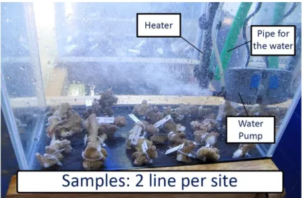
transcriptional levels of corals under field conditions. The remaining 24 branches per site per depth were randomly divided in groups of three branches, placed in eight experimental aquaria (Figure n.3.6) filled with 20L of natural sea water, and maintained with a movement pump (75 l/h) and continuous oxygenation. Corals spent a 14-days period of acclimatization to the laboratory conditions; in particular, a constant water temperature of 28 °C ± 0.5 °C close to the mean value at the collection sites was employed along with a natural photoperiod ( light-dark cycle, 10L:14D). The aquaria were filled through a system of two 150-L tanks which were constantly filled with seawater taken on-site at ~100 m from the shore (Figure n.3.7a and b). To prevent the stagnation, the water was moved by movement pump. It was not necessary to use a filtering system because the water was gradually but constantly flowed through the aquaria with a complete water change every 6 hours, so that the elimination of metabolites was constant while maintaining unchanged the water parameters, which were monitoring every 6 hours through a multi-parametric instrument (ADWA AD12) and densimeter (Milwaukee MR100 ATC).
After the acclimatization period, coral samples were collected from each treatment condition to accounted for animal physiological status at the onset of the experimental exposure to increased water temperature, thus representing the “zero time” (T0) of the time-course evaluation. At the onset of the experiments, aquaria were randomly divided in two groups of controls (temperature 28 °C ± 0.5°C) and thermally-challenged corals, in which water temperature was elevated at 31 °C ± 0.5 °C according to Barshis et al. (2013) and Kenkel et al. (2013). The experimental treatment were brought to 31 °C ± 0.5 °C over 12 h during the day, after which the temperature was reduced to ambient condition of 28 °C ± 0.5°C over 12 h during the darkness according to Mayfield et al. 2013.
Samplings were performed after 3 days and 7 days of exposure to the increased temperatures both in controls and thermally-challenged corals, and samples were immediately preserved in the RNAlater® solution (Sigma-Aldrich) and stored at – 20 °C until subsequent analysis. Four replicates were employed for each experimental condition (N = 4).
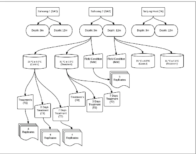
Figure n.3.6 - Experimental design flow chart. All the procedures were developed for each site (SA1, SA2, TA). Small branches of P. verrucosa were collected from 28 different coral colonies from each of the three different sites (SA1, SA2, TA) at each established depth (3 m and 12 m). Five randomly selected branches for each site and depth were immediately immersed in RNALater® to further assess transcriptional levels showed by corals under field conditions. The remaining 24 branches per site per depth were randomly divided in groups of three branches and placed in eight experimental aquaria (4 each experimental condition).
T0 are coral samples collected at the onset of the experimental exposure to increased water temperature and representing the “zero time”. T3 and T7 are the coral samples collected after respectively 3 and 7 days of exposure to the experimental conditions (31 °C ± 0.5 °C over 12 h during the day, 28 °C ± 0.5°C over 12 h during the darkness.
Figure n.3.8 b – Scheme of the setup of the aquariums ( Davide Poli 2014)
3.3 RNA Extraction and cDNA preparation
A small piece of coral branch (about 1 cm3) was mechanically homogenized in a
suitable volume of the Tri-Reagent® (Sigma Aldrich), and total RNA was extracted according to the manufacture’s protocol (Sigma Aldrich). The total RNA was resuspended in a suitable volume of DEPC-treated molecular-grade milliQ water (Life Technologies, Milan, Italy). RNA concentration and quality were verified using the Qubit RNA assay (Life Technologies, Milan, Italy) and electrophoresis using a 1.2% agarose gel under denaturing conditions. First strand cDNA for each sample was synthesized from 600 ng total RNA using the iScript supermix following manufacturer’s protocol (Biorad Laboratories, Milan, Italy). cDNA samples were further stored at – 20°C until analysed.
3.4 Real time PCR assays
Transcriptional analyses were conducted using Real Time quantitative Polymerase Chain Reaction (qPCR) assays. Expression levels of three target transcripts were evaluated in P. verrucosa; these transcripts encode an ATP synthase (ATPs), a NADH dehydrogeanse (NDH) and a 70kDa heat-shock protein (HSP70). Target specific primers were designed using Primer Express (Life Technologies, Milan, Italy) using nucleotide retrieved from the GeneBank database (https://www.ncbi.nlm.nih.gov/genbank/) for P. verrucosa (Table n.3.2).
Table n.3.2
Transcript Abbreviation GeneBank
Ac. Numb
Tm (°C) qPCR
Efficiency
ATP synthase ATPs JX985612 60°C 122.60%
NADH dehydrogenase
NDH Primer pair was deduced*
from a partial sequence of
P. damicornis (GeneBank Accession DQ351262) 60°C 120.06% Heat Shok Proteine 70kDa
HSP70 Primer pair was deduced*
from a partial sequence of
P. damicornis (GeneBank
Accession JX624896.1)
60°C 118.26%
*sequences actually under submission process to the GeneBank database
The qPCR technique is based on real-time monitoring of amplicon formation by a reporter molecule (e.g., SYBR green dye). Fluorescence is measured after each temperature cycle and is proportional to the amount of synthesized amplicon. The exponential growth of the amplicon concentration in the reaction mixture is described as an exponential function of the template starting concentration (Bustin et al. 2004). Two parameters are essential for
quantification: the threshold cycle, CT, and the qPCR efficiency (E). The CT is the number
of cycles necessary to reach a certain threshold fluorescence. In one experimental setup, the threshold is the same for all samples. Since fluorescence is a relative measure of the DNA content, samples containing higher amounts of target DNA will have lower CT, while samples holding lower amounts of target DNA will have higher CT values. E is a measure of amplification quality and depends on factors such as the primer GC content, primer mismatch, and the presence of PCR inhibitors. If E equals 2, the number of amplicons doubles per cycle, i.e., the efficiency is 100%.
At a first stage, we attempted to set-up a relative quantification protocol to infer changes
in mRNA expression of the selected transcripts. Relative quantification using the ΔΔCT
method is the most common method used in mRNA expression analyses (VanGuilder, et al. 2008). The method determines the expression ratio (or fold change) of a target transcript in a sample compared to a control, normalizing with the expression ratio of an internal
reference transcript, to control for sample-to-sample variations enabling comparisons of mRNA concentrations across different experimental conditions. Hypothetically, the ideal reference gene product is expressed at stable levels irrespective of tissue type, species, treatment, metabolism or sampling conditions, and computational approaches have to be used to infer suitability of a transcript as a putative reference transcript. According to the standardized guidelines (MIQE guidelines; Bustin et al., 2009), this is a mandatory pre-requisite for qPCR data publication in mammalian model species. Although in studies with non-model organisms, the lack of large set of genomic data has heavily limited these approaches, the increased awareness of the importance of systematic validation of reference gene selection is raised also considering the potential confounding factors given by environmental pressures on animal transcriptional profiles evaluated under field conditions (Maes et al. 2013).
We identified three candidate reference transcripts to be used in qPCR experiments with
P. verrucosa samples. These transcripts encoded the ribosomal proteins L22, L40 and P0.
Primers were designed basing on homologous sequences of P. damicornis. Representative PCR products for each gene product were cloned and sequenced to verify primer specificity in P. verrucosa (sequences are actually under submission process to the GeneBank database) Unfortunately, stability analysis performed using four different computational approaches (Franzellitti et al. submitted) showed that none of those selected transcripts were suitable as reference transcripts for qPCR data normalization in P. verrucosa under the experimental conditions employed in this study. As normalization is a critical step representing a relevant methodological bias in our transcriptional investigations with P.
verrucosa, we decided avoiding the semi-quantitative approach and going through the
application of absolute quantification protocols for the selected target gene products. Absolute quantification by the standard curve method employs a dilution series of known template concentrations (N0, expressed as copy numbers) in the qPCR assay. Linear
regression of log (N0) versus CT gives the standard curve, and this is then used to calculate
template concentrations, N0, of the samples. This method requires that E of the sample is the same as E of the standard.
qPCR standards for each target transcript were prepared by serial dilution of a purified and quantified PCR product to obtain a standard curve of Ct values vs the logarithmic DNA
Absolute mRNA abundance was calculated from the standard curves and expressed as copy
number/ng RNA (mean SEM).
Real-time PCR reactions were performed in duplicate, in a final volume of 10 µL containing 5 µL Fast Sybr Green reaction mix with ROX (Life Technologies, Milan, Italy), 2 µL diluted cDNA, and 0.2 µM specific primers (Table n). A control lacking the DNA template (no template) and a minus-reverse transcriptase (no RT) control were included in the real-time PCR analysis to determine the specificity of target cDNA amplification. Amplification was detected with a StepOne real time PCR system apparatus (Life Technologies, Milan, Italy) using a standard ‘‘fast mode’’ thermal protocol (Figure n 3.10). For each target mRNA, melting curves, gel pictures and sequences were further analysed to verify the specificity of the amplified products and the absence of artifacts. The amplification efficiency of each primer pair was calculated using a dilution series of samples cDNAs or of the qPCR standards (Table n).
Target: P.
verrucosa HSP70 Slope: -3.055
Y-Intercept:
31.036 R²: 0.996 Eff %: 112.503 Figure n.3.9 Example of a standard curve obtained for the HSP70 gene product of P. verrucosa. Blu squares represent the samples analyzed related to the standard curve; red squares represent the standards,
with 10-fold dilutions of a known concentration of template (10⁶-10⁻¹), on which the standard curve is constructed
Figure n.3.10 - Standard “fast mode” qPCR thermal protocol
3.5 Statistical analyses
Data were analyzed using the SigmaStat statistical package (SPSS Science, ver.3.1). Significant differences between samples were determined using 1-way ANOVA followed by the multiple comparison Bonferroni’s test. Statistical differences were accepted when p < 0.05.
Factor Analysis using the Principal Component Analysis extraction procedure was performed using the STATISTICA software package (StatSoft) to determine whether coral sampled in different sites and/or at different depths can be discriminated by means of overall variations of mRNA transcriptional profiles.
Clustering of qPCR data was performed to create heatmaps using the Gene Cluster software ver2.0 (Eisen, M. B. et al 1998) and the TreeView software for cluster visualizations. Both software packages are specifically written for the analysis of mRNA expression patterns obtained from microarrays as well as qPCR assays. Similarity was measured by standard correlation.
4 RESULTS
Summary
Transcriptional profiles under field conditions
Effects of the acclimatization to the laboratory conditions
Transcriptional-responses following P. verrucosa exposure to seawater
temperature increase under laboratory conditions
Cluster analysis Hsp70 mRNA expression Treatment ctr 3 days 7 days m R N A ex p res si o n ( fo ld ch an g e) 0,0 0,5 1,0 1,5 2,0 2,5 3,0 3,5 A LOW DEPTH A HIGH DEPTH B LOW DEPTH B HIGH DEPTH C LOW DEPTH C HIGH DEPTH