A
A
l
l
m
m
a
a
M
M
a
a
t
t
e
e
r
r
S
S
t
t
u
u
d
d
i
i
o
o
r
r
u
u
m
m
–
–
U
U
n
n
i
i
v
v
e
e
r
r
s
s
i
i
t
t
à
à
d
d
i
i
B
B
o
o
l
l
o
o
g
g
n
n
a
a
DOTTORATO DI RICERCA IN
BIOINGEGNERIA
Ciclo XXV
Settore Concorsuale di afferenza: 09/G2 Settore Scientifico disciplinare: ING–INF/06
TITOLO TESI
Methods for the Estimation of the Cortical Activity and
Connectivity during Cognitive Tasks in Humans
Presentata da: JLENIA TOPPICoordinatore Dottorato
Relatore
Prof. Angelo Cappello
Prof.ssa Serenella Salinari
Università di Bologna “Alma Mater Studiorum”
Università degli Studi di Roma “La Sapienza”
Corso di Dottorato di Ricerca in Bioingegneria – XXV ciclo
Coordinatore: Prof. Angelo Cappello
A.A. 2011/2012
Settore Scientifico/Disciplinare ING-INF/06
TESI DI DOTTORATO
METHODS FOR THE ESTIMATION OF CORTICAL
ACTIVITY AND CONNECTIVITY DURING COGNITIVE
TASKS IN HUMANS
Candidato: Ing. Jlenia Toppi
Supervisore: Prof.ssa Serenella Salinari
Co-Supervisore: Ing. Laura Astolfi
Controrelatori: Prof. Mauro Ursino
Table of Contents
GENERAL INTRODUCTION ... 5
SECTION I: STATISTICAL ASSESSMENT OF STATIONARY FUNCTIONAL CONNECTIVITY PATTERNS ESTIMATED ON NON-INVASIVE EEG MEASURES
INTRODUCTION ... 9
STATISTICAL ASSESSMENT OF CONNECTIVITY PATTERNS: STATE OF THE ART ... 13
Multivariate Methods for the Estimation of Connectivity 13
Partial Directed Coherence 13
Statistical tests for the assessment of connectivity patterns 15
Shuffling Method: Empirical Distribution 17
Asymptotic Statistic Method: Theoretical Distribution 17
Reducing the occurrence of Type I errors in assessment of connectivity patterns 18
False Discovery Rate 19
Bonferroni adjustment 19
COMPARING METHODS FOR THE STATISTICAL ASSESSMENT OF CONNECTIVITY PATTERNS: A SIMULATION STUDY ... 21
The Simulation Study 21
Signal Generation 22 Evaluation of performances 23 Statistical Analysis 24 Results 26 Discussion 36 CONCLUSION ... 39 SECTION I REFERENCES ... 41
SECTION II: TIME-VARYING APPROACH FOR THE ESTIMATION OF FUNCTIONAL CONNECTIVITY
INTRODUCTION ... 44
ESTIMATION OF TIME-VARYING FUNCTIONAL CONNECTIVITY: STATE OF THE ART ... 47
Adaptive Partial Directed Coherence 47
The Recursive Least Square 47
The General Linear Kalman Filter 49
COMPARING METHODS FOR THE ESTIMATION OF TIME-VARYING FUNCTIONAL CONNECTIVITY: A SIMULATION STUDY ... 51
The Simulation Study 51
Signal Generation 52
Statistical Analysis 57
Results 58
Discussion 67
CONCLUSION ... 70 SECTION II REFERENCES ... 72
SECTION III: GRAPH THEORY APPROACH: A CONSISTENT DESCRIPTION OF THE RELEVANT PROPERTIES OF THE BRAIN NETWORKS
INTRODUCTION ... 73 GRAPH THEORY APPROACH: STATE OF THE ART ... 76
Concept at the basis of Graph Theory 76
Adjacency Matrix Extraction 77
Graph Theory Indexes 77
BEYOND THE STATE OF THE ART: HOW THE STATISTICAL VALIDATION OF FUNCTIONAL CONNECTIVITY PATTERNS CAN PREVENT ERRONEOUS DEFINITION OF SMALL-WORLD PROPERTIES OF A BRAIN CONNECTIVITY NETWORK ... 81
Methods 82
Datasets used in the experiment 82
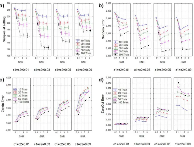
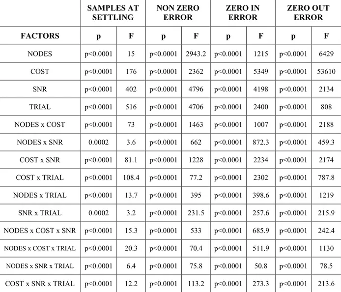
Signal Processing 83 Analysis of Variance 84 Results 84 Simulated data 84 Mannequin data 89 Discussion 93 CONCLUSION ... 96 SECTION III REFERENCES ... 98
SECTION IV: FUNCTIONAL CONNECTIVITY FOR THE STUDY OF RESTING STATE AND COGNITIVE PROCESSES IN HUMAN
INTRODUCTION ... 103 DESCRIBING RELEVANT INDEXES FROM THE RESTING STATE ELECTROPHYSIOLOGICAL NETWORKS ... 105
Introduction 105
Material and Methods 106
Experimental Design 106
Pre-Processing and Functional Connectivity Analysis 106
Results 107
Discussion 111
Introduction 113
Material and Methods 114
Experimental Design 114
Visual Oddball Task 114
Sternberg Task 115
Pre-Processing of EEG traces 117
Results 117
EEG Visual Oddball Task 117
EEG Sternberg Task 124
Discussion 131
CONCLUSION OF SECTION IV ... 133 SECTION IV REFERENCES ... 134 GENERAL CONCLUSION ... 136
5
General Introduction
The development of a methodology for the estimation of the information flow between different and differently specialized cerebral areas, starting from non-invasive measurements of the neuro-electrical brain activity, has gained more and more importance in the field of Neuroscience, as an instrument to investigate the neural basis of cerebral processes. In fact, the knowledge of the complex cerebral dynamics underlying human cognitive processes cannot be fully achieved by the reconstruction of temporal/spectral activations of different parts of the brain. The description of the brain circuits involved in the execution of a task is a crucial point for understanding the mechanisms at the basis of the specific function under examination, as well as for the development of applications in the clinical and rehabilitation fields.
In the last two decades, several approaches were developed and applied to neuroelectrical signals in order to estimate the connectivity patterns elicited among cerebral areas. Several studies investigated the properties of all the available methods providing different solutions for different application fields and highlighting the best approaches able to reproduce the brain circuits related to non-invasive EEG measurements.
The theory of Granger Causality (1969), based on the statistical studies on causality by Norbert Wiener (1956), is one of the most generally adopted in EEG based connectivity studies, due to its many advantages in terms of generality, easiness, and possibility to provide a fully multivariate analysis of brain circuits in terms of existence, strength, direction of the functional links. At the same time, this method avoids the necessity of a priori information on the brain circuits under investigation. Since it provides not a mere description of a synchronicity between distant brain structures, but an hypothesis on the brain circuits, including the influence exerted by a neural system to the others, it can be considered an estimator of the so-called effective connectivity.
Notwithstanding the advancements provided in this respect during the last twenty years, the main problem still unsolved regards the stability and reliability of the connectivity patterns obtained from Granger Causality-based approaches. Such issue still needs to be solved in order to provide an instrument really able to fulfill clinical and applicative purposes, where the reliability of the results and their consistence among the population are mandatory.
6
For this reason, my main aim during the three years of my PhD course was to study, develop and refine methodologies for effective connectivity estimation allowing to overcome the limitations of existent procedures with the aim to produce a valid tool able to reliably describe human connectivity networks and their global and local properties in different application fields.
The main aims of my PhD thesis can be summarized by two main goals: 1. METHODOLOGICAL AIMS
Development of a stable, consistent and reproducible procedure for effective connectivity estimation with a high impact on neuroscience field in order:
1. To avoid the a priori selection of the channels or brain regions to be included in the model
2. To assess the significance of functional connections, including the corrections for multiple comparisons
3. To consistently describe relevant properties of the brain networks
4. To accurately describe the temporal evolution of effective connectivity patterns
2. APPLICATIVE AIMS
1. Testing the new methodologies on real data in order to evaluate their application field.
2. to find quantifiable descriptors, based on brain connectivity indexes, of resting condition and cognitive processes (attention, memory)
In order to reach these two main goals I followed the roadmap reported in the figure below. In particular, the first year was dedicated to the study of the state of the art of all methodologies for effective connectivity estimation and to the refining of existent approaches for the estimation of connectivity patterns in the stationary case, i.e. when the statistical properties of the data can be considered stable during the observation window of our experiments. During the second year I faced the problem of statistically validating the estimated connectivity patterns, by comparing the existent assessing methodologies in an extensive simulation study with the aim to understand which was the best approach to be used in relation to the quality of the available data. Moreover, for the first time in connectivity field, I introduced corrections for multiple comparisons in the statistical validation process in
7
order to avoid the occurrence of false positives which might affect the topology of validated connectivity networks. The third year was dedicated to three important issues regarding the necessities i) to include all the sources in the model used for connectivity estimation, ii) to follow the temporal dynamics of connectivity patterns with a time varying approach and iii) to reliably extract indexes characterizing in a stable way the main properties of investigated networks.
The structure of the thesis reflects the route followed during these three years with the aim to produce a valid tool able to consistently and reliably estimate connectivity patterns and investigate their properties.
In Section I, after a description of the state of the art of stationary connectivity, an extensive simulation study aiming at comparing the two existent assessing methods under different conditions of data quality was described.
In Section II, a simulation study comparing the two more advanced methodologies for the estimation of time-varying Granger Causality connectivity was proposed.
In Section III, after a brief introduction on the concepts at the basis of graph theory, a study demonstrating how the procedure for the extraction of graph indexes from the
8
connectivity matrix can affect the topological properties of the investigated networks was provided.
In Section IV, all the developed methodologies were tested on real data in two neuroscience applications regarding the investigation of resting state brain networks and cognitive processes such as attention and memory in humans.
Section I
Statistical assessment of stationary functional
connectivity patterns estimated on non-invasive
EEG measures
INTRODUCTION
STATISTICAL ASSESSMENT OF CONNECTIVITY PATTERNS: STATE OF THE ART Multivariate Methods for the Estimation of Connectivity
Partial Directed Coherence
Statistical tests for the assessment of connectivity patterns
Shuffling Method: Empirical Distribution
Asymptotic Statistic Method: Theoretical Distribution
Reducing the occurrence of Type I errors in assessment of connectivity patterns
False Discovery Rate Bonferroni adjustment
COMPARING METHODS FOR THE STATISTICAL ASSESSMENT OF CONNECTIVITY PATTERNS: A SIMULATION STUDY
The Simulation Study
Signal Generation Evaluation of performances Statistical Analysis Results Discussion CONCLUSION SECTION I REFERENCES _______________________________________________________________________________________________
Introduction
In neuroscience field, the concept of brain connectivity (i.e. how the cortical areas communicate one to each other) is central for the understanding of the organized behavior of cortical regions beyond the simple mapping of their activity (Horwitz, 2003; Lee et al., 2003). In the last two decades several studies have been carried on in order to understand neuronal networks at the basis of mental processes, which are characterized by lots of interactions between different and differently specialized cortical sites. Connectivity estimation techniques aim at describing interactions between electrodes or cortical areas as connectivity patterns
10
holding the direction and the strength of the information flow between such areas. The functional connectivity between cortical areas is then defined as the temporal correlation between spatially remote neurophysiologic events and it could be estimated by using different methods both in time as well as in frequency domain based on bivariate or multivariate autoregressive models (Blinowska, 2011; Kaminski and Blinowska, 1991; Sameshima and Baccalá, 1999; Turbes et al., 1983). Several studies have proved the higher efficiency in estimating functional connectivity of methods, such as Directed Transfer Function (DTF) (Kaminski and Blinowska, 1991) or Partial Directed Coherence (PDC) (Baccalá and Sameshima, 2001), which are defined in frequency domain and based on the use of multivariate autoregressive (MVAR) models built on original time-series (Kus et al., 2004). In fact the bivariate approach is affected by a high number of false positives due to the impossibility of the method in discarding a common effect on a couple of signals of a third one acquired simultaneously (Blinowska et al., 2004). Moreover the bivariate methods give rise to very dense patterns of propagation, thus it is impossible to find the sources of propagation (Blinowska et al., 2010; David et al., 2004). The PDC technique has been demonstrated (Baccalá and Sameshima, 2001) to rely the concept of Granger causality between time series (Granger, 1969), according to which an observed time series x(n) causes another series y(n) if the knowledge of x(n)’s past significantly improves prediction of y(n). Moreover, the PDC is also of particular interest because it can distinguish between direct and indirect connectivity flows in the estimated connectivity pattern better than Directed Transfer Function (DTF) and its direct modified version, the dDTF (Astolfi et al., 2007).
Random correlations between signals induced by environmental noise or by chance can lead to false detection of links or to the loss of true existing connections in the connectivity estimation process. In order to minimize this phenomenon, the process of functional connectivity estimation has to be followed by a procedure able to assess the statistical significance of estimated networks, distinguishing the estimated connectivity patterns from the null case. As PDC functions have a highly nonlinear relation to the time series data from which they are derived, the distribution of such estimator in the null case has not been well established for several years. Therefore, several methods have been introduced in order to build the PDC distribution in an empirical way (Kaminski et al., 2001; Sameshima and Baccalá, 1999). The first one, the Spectral Causality Criterion, consisted in the use of the threshold value 0.1 for all the connections, directions and frequency samples included in the analysis (Sameshima and Baccalá, 1999). Its non-dependence from the data subjected to effective connectivity analysis led to the development of a data-driven approach, the shuffling
11
procedure, able to empirically build the null-case distribution by shuffling the phase of the investigated signals. Such approach had the advantage to increase the accuracy of estimation approach but at the same time the disadvantage to reduce the speed of validation process, being based on a time consuming approach. Only in 2007 the real distribution of PDC in the null-case was asimptotically theorized (Takahashi et al., 2007), allowing to increase the accuracy of validation process and reducing the computational time required for empirical methods.
All the assessing methods required the definition of a significance level to be applied in order to evaluate the statistical threshold for each possible connection between signals in the multivariate dataset and for each frequency sample. Due to the high number of statistical assessments performed simultaneously, it is necessary to apply corrections to the significance level imposed in the validation process, in order to prevent the occurrence of type I errors (Nichols and Hayasaka, 2003). In fact, statistical theory offers a lot of solutions for adequately manage the occurrence of type I errors during the execution of multiple univariate tests, such as the traditional Bonferroni adjustment (Bonferroni, 1936) or the more recent False Discovery Rate (FDR) (Benjamini and Yekutieli, 2001; Benjamini and Hochberg, 1995). Even if the Shuffling method for statistical validation of connectivity patterns has been proposed in literature since 2001, a comprehensive analysis of its performances under different conditions of signal-to-noise ratio (factor SNR) and signal lengths (factor LENGTH) was not available in literature before my PhD. In addition, the definition of a new assessing method allowed to make comparisons between the two procedures in terms of percentages of type I and type II errors occurred during the validation process in order to highlight the best assessing procedure to be applied also in relation with the quality (SNR level) and amount of available data. Moreover, for the first time in the functional connectivity field, I proposed the introduction of corrections for multiple comparisons in the assessment process of connectivity patterns, also studying their effects on the validated networks.
In the present section of my thesis, first of all I briefly describe the methods available at the moment for assessing the estimated functional connectivity patterns and for adjusting the significance level of statistical test by taking into account multiple comparisons. This overview was followed by a description of the simulation study performed in order to compare the performances achieved by the two validation methods in terms of both false positives and false negatives under different condition of signal to noise ratio (SNR) and
12
amount of data available for the analysis. In particular the study allowed to address the following specific questions:
1) Is the Shuffling procedure a reliable method for preventing the occurrence of type I and type II errors?
2) How the statistical corrections for multiple comparisons affect the performances of Shuffling procedure?
3) Known the high computational complexity of the procedure based on empirical reconstruction of null-case distribution (shuffling), can the method based on its theoretical definition (Asymptotic Statistic) substitute it in the assessment of connectivity patterns?
4) Does the definition of PDC estimator (normalization according to columns or rows) influence the performances of the two assessing methods?
5) How are the performances of the two methods influenced by different factors affecting the recordings, like the signal-to-noise ratio (factor SNR) and the amount of data at disposal for the analysis (factor LENGTH)?
In order to answer these questions, a simulation study was performed, on the basis of a predefined connectivity scheme which linked several modeled cerebral areas. Functional connections between these areas were retrieved by the estimation process under different experimental SNR and LENGTH conditions. Analysis of variance (ANOVA) and Duncan’s pairwise comparisons were applied in order to: i) evaluate the effect of different factors such as SNR and data length on the percentages of false positives and false negatives occurred during the validation process; ii) compare the existent Shuffling procedure with the new Asymptotic Statistic approach in order to understand the best assessing method also in relation to the quality of data available for the analysis.
Statistical Assessment of Connectivity Patterns: State of
the Art
Multivariate Methods for the Estimation of Connectivity
Let Y be a set of signals, obtained from non-invasive EEG recordings or from the reconstruction of neuro-electrical cortical activities based on scalp measures:
T N t y t y t y Y =[ 1( ), 2( ),..., ( )] (1.1) where t refers to time and N is the number of electrodes or cortical areas considered.
Supposing that the following MVAR process is an adequate description of the dataset Y:
∑
= = − Λ p k t E k t Y k 0 ) ( ) ( ) ( with Λ(0)=I (1.2)where Y(t) is the data vector in time, E(t) = [e1(t),…,en(t)]T is a vector of multivariate
zero-mean uncorrelated white noise processes, Λ(1),Λ(2),…,Λ(p) are the NxN matrices of model coefficients and p is the model order, usually chosen by means of the Akaike Information Criteria (AIC) for MVAR processes (Akaike, 1974).
Once an MVAR model is adequately estimated, it becomes the basis for subsequent spectral analysis. To investigate the spectral properties of the examined process, Eq. (1.2) is transformed to the frequency domain:
) ( ) ( ) (f Y f =E f Λ (1.3) where:
∑
= ∆ − Λ = Λ p k tk f j e k f 0 2 ) ( ) ( π (1.4)and Δt is the temporal interval between two samples.
Partial Directed Coherence
The Partial Directed Coherence (PDC) (Baccalá and Sameshima, 2001) is a full multivariate spectral measure, used to determine the directed influences between pairs of signals in a multivariate data set. PDC is a frequency domain representation of the existing multivariate
14
relationships between simultaneously analyzed time series that allows the inference of functional relationships between them. This estimator was demonstrated to be a frequency version of the concept of Granger causality (Granger, 1969), according to which a time series x[n] can be said to have an influence on another time series y[n] if the knowledge of past samples of x significantly reduces the prediction error for the present sample of y.
It is possible to define PDC as
∑
= Λ Λ Λ = N k kj kj ij ij f f f f 1 * ( ) ) ( ) ( ) ( π (1.5)which bears its name by its relation to the well-known concept of partial coherence (Baccalá, 2001). The PDC from node j to node i, πij(f), describes the directional flow of information
from the signal yj(n) to yi(n), whereupon common effects produced by other signals yk(n) on
the latter are subtracted leaving only a description that is exclusive from yj(n) to yi(n). PDC
squared values are in the interval [0;1] and the normalization condition
1 ) ( 1 2 =
∑
= N n nj f π (1.6)is verified. According to this normalization, πij(f) represents the fraction of the information
flow of node j directed to node i, as compared to all the j’s interactions with other nodes. Even if this formulation derived directly from information theory, the original definition was modified in order to give a better physiological interpretation to the estimate results achieved on electrophysiological data. In particular, a new type of normalization, already used for another connectivity estimator such as Directed Transfer Function (Kaminski and Blinowska, 1991) was introduced. Such normalization consisted in dividing each estimated value of PDC for the root squared sums of all elements of the relative row, obtaining the following definition:
∑
= Λ Λ Λ = N k ik ik ij row ij f f f f 1 * ( ) ) ( ) ( ) ( π (1.7)Even in this formulation PDC squared values are in the range [0;1] but the normalization condition is as follows:
15 1 ) ( 1 2 =
∑
= N n row in f π (1.8)Moreover, a squared formulation of PDC has been introduced and can be defined as follows for the two types of normalization:
∑
= Λ Λ = N k kj ij col ij f f f sPDC 1 2 2 ) ( ) ( ) ( (1.9)∑
= Λ Λ = N k ik ij row ij f f f sPDC 1 2 2 ) ( ) ( ) ( (1.10)The main difference with respect to the original formulation is in the interpretation of these estimators. Squared PDC can be put in relationship with the power density of the investigated signals and can be interpreted as the fraction of ith signal power density due to the jth measure. The higher performances of squared methods in respect to simple PDC have been demonstrated in a simulation study. Such study revealed higher accuracy, for the methods based on squared formulation of PDC, in the estimation of connectivity patterns on data characterized by different lengths and signal to noise ratio (SNR) and in distinction between direct and indirect pathways (Astolfi et al., 2006).
Statistical tests for the assessment of connectivity patterns
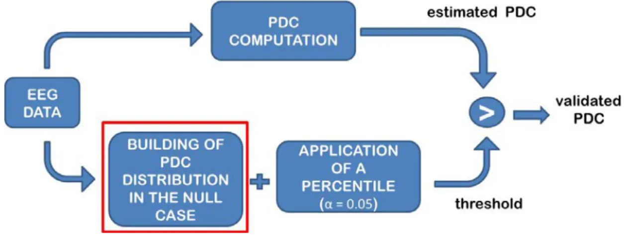
Random correlation between signals induced by environmental noise or by chance can lead to the presence of spurious links in the connectivity estimation process. In order to assess the significance of estimated patterns, the value of functional connectivity for a given pair of signals and for each frequency, obtained by computing PDC, has to be statistically compared with a threshold level which is related to the lack of transmission between considered signals (Fig. 1.1). Due to the high nonlinear dependence of the PDC from the estimated MVAR parameters, the theoretical distribution for such estimator in the null case has been not known until few years ago. For this reason different procedures for empirically reconstructing the distribution of the PDC in the null case (absence of connection) were developed in order to extract statistical thresholds to be compared with the inferred patterns by means of statistical tests for a fixed significance level α.
16
Figure 1.1 – Flow-chart describing the statistical validation process of functional connectivity
The first assessing method was introduced by Schnider for the directed coherence estimator (Schnider et al., 1989) and then was applied to PDC by Sameshima and Baccalà (Sameshima and Baccalá, 1999) with the name of Spectral Causality Criterion (SCC). It consists in the use of the same threshold, set to 0.1, for all the frequencies and for all the couples and directions, below which the connectivity value is considered due to chance. This criterion, which is simplex to be applied and does not require any computation, has been demonstrated corresponding to the application of a percentile of 99% on the null case distribution achieved empirically by estimating functional connectivity on simulated couples of independent white noise (Gourévitch et al., 2006).
In order to improve the accuracy of the validation process, new methods based on the computation of a significance threshold, depending on the data, for each link and for each frequency were developed. The shuffling is a time consuming procedure, introduced in 2001 (Kaminski et al., 2001), which allows to achieve a distribution for the null case by iterating the PDC estimation on different surrogate data sets obtained by shuffling the original traces in order to disrupt the temporal relations between them. The shuffling procedure may involve the phases of the signals in the frequency domain or the samples of data in time domain (Faes et al., 2009). The necessity to reduce the time required for the computation of statistical thresholds in Shuffling procedure, led to the development of a recent validation approach based on the theoretical distribution of the PDC, which tends asymptotically to a χ2
-distribution in the null case (lack of transmission) (Takahashi et al., 2007; Schelter et al., 2006). A detailed description of the two validation procedures can be found below.
17
Shuffling Method: Empirical Distribution
Shuffling method is based on the generation of sets of surrogate data (Theiler et al., 1992), obtained shuffling the time series of each channel. Data shuffling can be computed in different ways, although the most used is the phase shuffling. In particular, original data are transformed from time domain to frequency domain by means of Fourier Transform; the data phases are mixed without modifying their amplitude and shuffled signals are taken back in the time domain. This procedure is able to save the amplitude of the power spectrum, but at the same time to disrupt causal links between signals. A MVAR model is fitted to surrogate data set and connectivity estimates are derived from the model. Iterating this process many times, each time on a new surrogate data set, allows to build an empirical distribution of the null hypothesis for the causal estimator (Kamiński et al., 2001). Once obtained the empirical distribution, the significance of the estimated connectivity patterns for a fixed significance level is assessed. In particular, the threshold value, below which the estimated connection is due to the case, is evaluated for each couple of signals and for each frequency by applying a percentile, corresponding to a predefined significance level, on the null-case empirical distribution computed for the correspondent link. The only connections whose values exceed the thresholds are considered as not due to the case.
Asymptotic Statistic Method: Theoretical Distribution
The only way to reduce the computational time required for statistical assessment process and to improve its accuracy is to use the theoretical distribution of FC for the null case instead building its empirical approximation by a time consuming procedure. Recently, Schelter et al. introduced the concept that PDC estimator for the not-null hypothesis is asymptotically normally distributed, while it tends to a χ2-distribution in the null case (Schelter et al., 2006). Relying on this statement, it is possible to derive the null-case distribution of PDC from the acquired signals by applying a Monte Carlo method able to reshape the data on a χ2 -distribution to be used in the assessment process. Details about the method can be found in Takahashi et al. (Takahashi et al., 2007). Once obtained the null case distribution, the procedure of validation is applied as already explained in the previous section for the shuffling method.
18
Reducing the occurrence of Type I errors in assessment of connectivity
patterns
The statistical validation process has to be applied on each couple of signals for each direction and for each frequency sample. This necessity leads to the execution of a high number of simultaneous univariate statistical tests with evident consequences in the occurrence of type I errors. The statistical theory provides several techniques that could be usefully applied in the context of the assessment of connectivity patterns in order to avoid the occurrence of false positives.
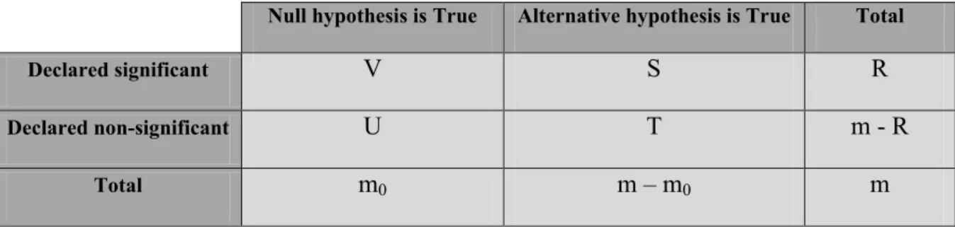
The family-wise error rate represents the probability of observing one or more false positives after carrying out simultaneous univariate tests. Supposing to have m null hypotheses H1, H2, ..., Hm. Each hypothesis could be declared significant or non-significant by means of a
statistical test. Tab.1.1 summarizes the situation after multiple significance tests are simultaneously applied:
Null hypothesis is True Alternative hypothesis is True Total
Declared significant V S R
Declared non-significant U T m - R
Total m0 m – m0 m
Table 1.1 – Table explaining the concept of family-wise error rate
where:
- m0 is the number of true null hypotheses
- m-m0 is the number of true alternative hypotheses
- V is the number of false positives (Type I error) - S is the number of true positives
- T is the number of false negatives (Type II error) - U is the number of true negatives
- R is the number of rejected null hypotheses
The FWER is the probability of making even one type I error in the family:
) 1 Pr( ≥
= V
19
Many methodologies are available for preventing type I errors (Nichols and Hayasaka, 2003), but in the following sections I limit the discussion to False Discovery Rate (FDR) and Bonferroni adjustments, which are the most used methodologies in neuroscience field.
False Discovery Rate
The false discovery rate (FDR), suggested by Benjamini and Hochberg (1995) is the expected proportion of erroneous rejections among all rejections. Considering V as the number of false positives and S as the number of true positives, the FDR is given by:
+ = S V V E FDR (1.12)
where E[] is the symbol for expected value.
In the following I reported the False Discovery Rate controlling procedure described by Benjamini and Hochberg in 1995. Let H1, H2,…, Hm be the null hypotheses, with m as the
number of univariate tests to be performed, and p1, p2, …, pm their corresponding p-values.
Let order in ascending order the p-values as p(1) ≤ p(2) ≤ … ≤ p(m) and then select the largest i (i=k) for which the condition
α m
i
P(i) ≤ (1.13)
is verified.
At the end, the hypotheses Hi with i=1, …, k have to be rejected.
In the case of independent tests, an approximation for evaluating corrected significance level has been introduced (Benjamini and Hochberg, 1995; Benjamini and Yekutieli, 2001):
α β m m 2 ) 1 ( * = + (1.14)
In this case the new level of significance is β*. Such value guarantees that each test is
performed with the imposed significance α.
Bonferroni adjustment
The Bonferroni adjustment (Bonferroni, 1936) starts from the consideration that if I perform N univariate tests, each one of them with an unknown significant probability α, the probability p that at least one of the test is significant is given by (Zar, 2010):
α
N
20
In other words this means that if N = 20 tests are performed with the usual probability α = 0.05, at least one of them became significant statistically by chance alone. However, the Bonferroni adjustment required that the probability p for which this event could occur (i.e., one result will be statistically significant by chance alone) could be equal to α. By using the Eq. (1.15), the single test will be performed at a probability
N
/
*
α
β
= (1.16)This β* is the actual probability at which the statistical tests are performed in order to conclude that all of the tests are performed at α level of statistical significance, Bonferroni adjusted for multiple comparisons. The Bonferroni adjustment is quite flexible since it does not require the hypothesis of independence of the data to be applied.
21
Comparing Methods for the Statistical Assessment of
Connectivity Patterns: A Simulation Study
The Simulation Study
In order to compare the two methodologies available at the moment for assessing the significance of connectivity patterns, I performed a simulation study in which the performances achieved for the two methods were evaluated under different conditions of SNR and amount of data available for the analysis.
The simulation study was composed by the following steps:
1) Generation of several sets of test signals simulating activations at scalp or cortical levels. These datasets were generated in order to fit a predefined connectivity model and to respect imposed levels of some factors. These factors were the SNR (factor SNR) and the total length of the data (factor LENGTH).
2) Estimation of the cortical connectivity patterns obtained in different conditions of SNR and data LENGTH by means of sPDCcol (squared PDC normalized according to columns), sPDCrow (squared PDC normalized according to rows) and sPDCnn (squared PDC not normalized). The normalization was applied before and after the validation process (factor NORMTYPE).
3) Application of the two different methods, the shuffling and asymptotic statistic procedures (factor VALIDTYPE), for assessing significance of estimated connectivity patterns. The evaluation of significant thresholds in both methods was computed applying a significance level of 0.05 in three different cases: no correction, corrected for multiple comparisons by means of FDR and Bonferroni adjustments (factor CORRECTION).
4) Computation of the total percentage of false positives and false negatives occurred in the assessment of significance of connectivity patterns for all the considered factors. 5) Statistical analysis of percentage of both false positives and negatives by means of
ANOVA for repeated measures in order to evaluate the effects of some factors (SNR, LENGTH, CORRECTION, NORMTYPE ) on the performances achieved by means of the two validation methods.
22
Signal Generation
Different simulated datasets were generated fitting a predefined model, which is reported in Fig. 1.2, composed by 4 cortical areas and imposing different levels of Signal to Noise Ratio (factor SNR) and data length (factor LENGTH).
Figure 1.2 - Connectivity model imposed in the generation of testing dataset. x1,…, x4 represent the signals of four
electrodes or cortical regions of interest. aij represents the strength of the imposed connection between nodes i and j,
while τij represents the delay in transmission applied between the two signals xi and xj in the generation of the dataset.
The values chosen for connections strength are a12=0.5, a13=0.4 a14=0.2, a23=0.08, while the values set for delays in
transmission are τ12=10s, τ13=10s, τ14=5s, τ23=20s at sampling rate of 200Hz.
x1(t) is a real signal acquired at the scalp level during a high resolution EEG recording session
(61 channels) involving a healthy subject during the rest condition. The other signals x2(t), …, x4(t) were iteratively achieved according to the predefined scheme reported in
Fig. 1.2. In particular, the signal xj(t) is obtained adding uncorrelated Gaussian white noise to
all the contributions of other signals xi(t) (with i≠j), each of which amplified of aij and delayed
of τij. The scheme is composed by 3 direct arcs (1 → 2; 1 → 4; 2 → 3), a direct-indirect arc
(1 → 2 → 3) between node 1 and node 3 through node 2 and 8 “null” arcs, i.e. 8 pairs of ROIs which are not linked, not directly nor indirectly. Coefficients for connection strengths used in the imposed model are a12=0.5, a13=0.4 a14=0.2, a23=0.08. These values are chosen in a
realistic range which is typical of connectivity patterns estimated on data recorded during memory, motor and sensory tasks (Astolfi et al., 2009; Büchel and Friston, 1997). In particular the low value chosen for the connection between nodes 2 and 3 was introduced with the aim to test the accuracy of validation process even for weak connections. The values used for the delay in transmission are τ12=2, τ13=2, τ14=1, τ23=4 data samples which correspond to
τ12=10 ms, τ13=10 ms, τ14=5 ms, τ23=20 ms at a sampling rate of 200 Hz.
23 - SNR factor = [ 0.1; 1; 3; 5; 10]
- LENGTH factor = [3000; 10000; 20000; 30000] data samples corresponding to a signal length of [15; 50; 100; 150] s, at a sampling rate of 200 Hz.
The levels chosen for both SNR and LENGTH factors cover the typical range for the cortical activity estimated during high resolution EEG experiments.
The MVAR models was estimated by means of Nuttall-Strand method, or multivariate Burg algorithm, which is one of the most common estimators for MVAR models and has been demonstrated to provide the most accurate results (Marple, 1987; Kay, 1988; Schlögl, 2006).
Evaluation of performances
A statistical evaluation of accuracy in assessing significance of estimated connectivity patterns was required to compare the two considered validation methods. The accuracy was quantified by means of two indicators, which are the percentages of false positives and of false negatives committed during the statistical assessment of estimated networks. These percentages were obtained comparing the results of connectivity estimation with the imposed connection scheme.
The percentage of false positives was computed considering the number of nodes pairs between which the estimated connectivity value was significantly different from null case while the imposed value in the predefined model was zero (no connection). In particular the percentage of false positives (FP%) was defined as follows:
) ( ) , ( mod 1 % start end el f f f n n f f n f n FP end start TOT − ⋅ Κ = += = +
∑ ∑
(1.17)where [fstart fend] is the frequency range in which the PDC was computed, n+model is the number
of not “null” connections in the imposed model and K+(n,f) is
≤ − → > − → = + 0 )) , ( ) , ( ~ ( 0 0 )) , ( ) , ( ~ ( 1 ) , (n f aa nn ff aa nn ff K ij ij ij ij (1.18)
where ~aij(n,f) and aij( fn, ) are the boolean expressions for the estimated and the imposed PDC values respectively. In fact ~aij(n,f) is set to 1 when the PDC value for the link n and at frequency f exceeds the significance threshold and is set to 0 when PDC value for the link n and at frequency f is below the statistical threshold, while aij( fn, ) is set to 1 when the
24
imposed value is different from zero and is set to 0 when the imposed value in the model is zero.
The percentage of false negatives was computed considering the number of nodes pairs between which the estimated connectivity value was not significantly different from null case while its imposed value was different from zero in the predefined model. In particular the percentage of false negatives (FN%) was defined as follows:
) ( * ) , ( mod 1 % start end el f f f n n f f n f n FN end start TOT − Κ = −= = −
∑ ∑
(1.19)where [fstart fend] is the frequency range in which the PDC was computed, n-model is the number
of “null” connections in the imposed model and K-(n,f) is
≥ − → < − → = − 0 )) , ( ) , ( ~ ( 0 0 )) , ( ) , ( ~ ( 1 ) , (n f aa nn ff aa nn ff K ij ij ij ij (1.20)
where ~aij(n,f) and aij( fn, ) are the boolean expressions for the estimated and the imposed PDC values respectively, define as describe above.
Both indexes were computed for the two validation methods (factor VALIDTYPE), for different normalization types (factor NORMTYPE) and for a significance level of 0.05 not corrected and corrected with FDR and Bonferroni adjustments (factor CORRECTION).
Simulations were performed by repeating for 100 times each generation-estimation procedure, in order to increase the robustness of the following statistical analysis.
Statistical Analysis
The percentages of false positives and false negatives were subjected to separate ANOVAs. First, I performed a four-way ANOVA aiming at studying the effect of different normalizations applied to PDC spectral estimator (NORMTYPE) on the percentages of false positives and false negatives occurred during estimation process, taking into account several factors such as the SNR, the length of data used for the processing (LENGTH) and the use of different methods of corrections for multiple comparisons (CORRECTION). The within main factors of the ANOVA were NORMTYPE (with five levels: NoNorm → no normalization, NormRowPre → rows normalization before statistical validation, NormRowPost → rows normalization after statistical validation, NormColPre → columns normalization before statistical validation, NormColPost → columns normalization after statistical validation),
25
SNR (with five levels: 0.1, 1, 3, 5, 10), LENGTH (with four levels: [3000, 10000, 20000 30000] data samples, corresponding to a signal length of [15, 50, 100, 150] s, at a sampling rate of 200 Hz) and CORRECTION (with three levels: no correction, FDR and Bonferroni). The dependent variables were both the percentages of false positives and false negatives occurred during the validation process. Duncan’s pairwise comparisons were then performed in order to better understand the significance between different levels of the same factor or between different factors within the same level. This analysis was executed on the connectivity networks validated applying both Shuffling and Asymptotic Statistic procedures. The second analysis was a four-way ANOVA aiming at comparing the two validation procedures (VALIDTYPE) in terms of both percentages of false positives and false negatives occurred during estimation process, taking into account different factors such as the SNR, the length of the data subject to the processing (LENGTH) and the use of different methods of corrections for multiple comparisons (CORRECTION). The within main factors of the ANOVA were VALIDTYPE (with two levels: Shuffling and Asymptotic Statistic procedures), SNR (with five levels: 0.1, 1, 3, 5, 10), LENGTH (with four levels: [3000, 10000, 20000 30000] data samples, corresponding to a signals length of [15, 50, 100, 150] s, at a sampling rate of 200 Hz) and CORRECTION (with three levels: no correction, FDR and Bonferroni). The dependent variables were both the percentages of false positives and false negatives occurred during the validation process. Duncan’s pairwise comparisons were then performed. This analysis was executed on the connectivity patterns achieved by applying each type of normalization (rows, columns or none).
The third analysis was a four-way ANOVA aiming at comparing the two validation procedures (VALIDTYPE) in terms of percentages of false positives occurred during estimation process focalizing the attention on each link (LINK) and taking into account different factors such as the SNR, the length of data used for the processing (LENGTH) and the use of different methods of corrections for multiple comparisons (CORRECTION). The within main factors of the ANOVAs were LINK (with eight levels: 2→1, 3→1, 4→1, 3→2, 4→2, 4→3, 2→4, 3→4), SNR (with five levels: 0.1, 1, 3, 5, 10), LENGTH (with four levels: [3000, 10000, 20000 30000] data samples, corresponding to a signals length of [15, 50, 100, 150] s, at a sampling rate of 200 Hz) and CORRECTION (with three levels: no correction, FDR and Bonferroni). The dependent variable was the percentage of false positives occurred during the validation process. Duncan’s pairwise comparisons were then performed. This
26
analysis was executed on the connectivity patterns validated applying both Shuffling and Asymptotic Statistic procedure.
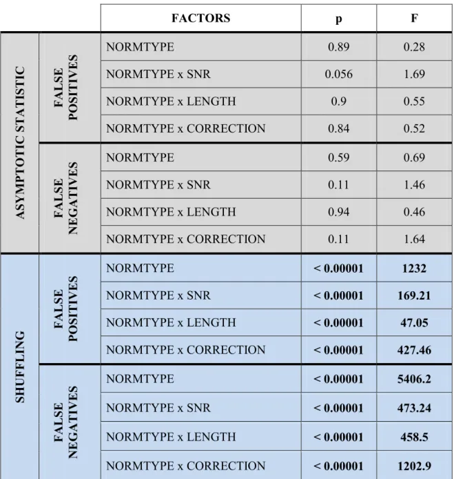
FACTORS p F A SY M PTO TI C S TA TI STI C FA LS E PO SIT IV E S NORMTYPE 0.89 0.28 NORMTYPE x SNR 0.056 1.69 NORMTYPE x LENGTH 0.9 0.55 NORMTYPE x CORRECTION 0.84 0.52 FA LS E NE G AT IVE S NORMTYPE 0.59 0.69 NORMTYPE x SNR 0.11 1.46 NORMTYPE x LENGTH 0.94 0.46 NORMTYPE x CORRECTION 0.11 1.64 SH UF FL ING FA LS E PO SIT IV E S NORMTYPE < 0.00001 1232 NORMTYPE x SNR < 0.00001 169.21 NORMTYPE x LENGTH < 0.00001 47.05 NORMTYPE x CORRECTION < 0.00001 427.46 FA LS E NE G AT IVE S NORMTYPE < 0.00001 5406.2 NORMTYPE x SNR < 0.00001 473.24 NORMTYPE x LENGTH < 0.00001 458.5 NORMTYPE x CORRECTION < 0.00001 1202.9
Table 1.2 – Results of the ANOVA performed on the percentages of false positives and false negatives occurred during the validation process executed by means of Asymptotic Statistic and Shuffling methods. The within main factors were the
normalization type (NORMTYPE), the signal to noise ratio (SNR), the data length (LENGTH) and the statistical corrections used for imposing the significance level (CORRECTION)
Results
Several sets of signals were generated as described in the previous section, in order to fit the connectivity pattern shown in Fig. 1.2. The imposed connectivity model contained three indirect arcs, one direct-indirect arc between nodes 1 and 3 through node 2 characterized by a
27
weak connection between nodes 2 and 3, and eight “null” arcs. This topology was chosen in order to test the performances of estimation/validation process in:
- preventing estimates of nonexistent arcs (false positives) - avoiding inversions of direct paths (false positives) - discarding existent links (false negatives)
- distinguishing real weak connections from links due to the case (false negatives) A MVAR model of order 16 was fitted to each set of simulated data, which were in the form of several trials of the same length (1s). The procedure of signal generation, estimation of connectivity patterns by means of sPDCnn, sPDCcol, sPDCrow and statistical validation for not corrected and adjusted statistical significance level 0.05 was carried out 100 times for each level of factors SNR and LENGTH, as indicated in the previous paragraphs, in order to increase the robustness of the subsequent statistical analysis.
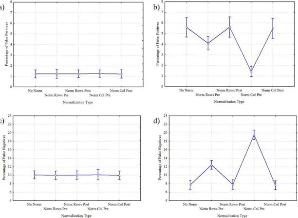
Figure 1.3 - Results of ANOVA performed on the percentages of false positives (first row) and false negatives (second row) occurred applying Asymptotic Statistic (first column) and Shuffling procedure (second column) respectively, using
NORMTYPE as within main factor. The diagram shows the mean value for the percentages obtained not normalizing and normalizing according to rows and columns, before and after the validation process the inferred connectivity
28
The indexes of performances used were the percentages of false positives and false negatives. They were computed for each generation-estimation procedure performed, and then subjected to different ANOVAs.
A four-way ANOVA was applied separately to the percentages of false positives and false negatives occurred during the validation process performed by means of Asymptotic Statistic and Shuffling procedures. The within main factors were the normalization type (NORMTYPE), the signal to noise ratio (SNR), the data length (LENGTH) and the statistical corrections used for imposing the significance level (CORRECTION). The corresponding results were reported in Tab.1.2. In particular they revealed no statistical influence of the main factor NORMTYPE on percentages of false positives and false negatives committed using Asymptotic Statistic validation procedure. Although high statistical influence of the main factors NORMTYPE and its interactions NORMTYPE x SNR, NORMTYPE x LENGTH, NORMTYPE x CORRECTION resulted on percentages of both false positives and false negatives occurred applying Shuffling validation method.
In Fig. 1.3 I reported results of ANOVA performed on the percentages of false positives (first row) and false negatives (second row) occurred with the application of Asymptotic Statistic (first column) and Shuffling procedure (second column) respectively, using NORMTYPE as within main factor. The diagram shows the mean value for the percentages obtained not normalizing and normalizing according to rows and columns, before and after the validation process, the inferred connectivity patterns. The bar represented their relative 95% confidence interval. Diagrams in the two columns of Fig. 1.3 revealed different behavior of the two validation methods in discarding both false positives and false negatives during the statistical assessment procedure in relation to the applied normalization type. In fact, panel a and c showed no significant differences, for Asymptotic Statistic method, between the normalization types in the percentages of type I and type II errors, which remained strictly around 1.2% and 10% respectively, as confirmed by Duncan’s pairwise comparisons. Panel b and d revealed a strong influence of the normalization type on the occurrence of type I and type II errors during the application of Shuffling method. In particular, in panel b, the percentage of false positives remained within the range [4% – 6%] except for the normalization according to columns applied before the validation procedure, for which the percentage highly decreased down to 1.5%. Duncan’s pairwise comparisons highlighted significant differences (p<0.00001) between the normalization types, with exceptions of the cases no normalization, normalization according to row and according to column both after
29
the validation method. In panel d, the percentage of false negatives ranged between 7.5% and 12% except for the case Normalization according to columns, for which the value reached the 20%. Duncan’s pairwise comparisons highlighted significant differences (p<0.00001) between the normalization types, with exceptions of the cases no normalization, normalization according to row and according to column both executed after the validation method.
FALSE POSITIVES FALSE NEGATIVES
FACTORS p F p F VALIDTYPE < 0.00001 3996 < 0.00001 625 SNR < 0.00001 762 < 0.00001 117 LENGTH < 0.00001 10 < 0.00001 11300 CORRECTION < 0.00001 6598 < 0.00001 10200 VALIDTYPE x SNR < 0.00001 549 < 0.00001 206 VALIDTYPE x LENGTH < 0.00001 7 < 0.00001 35 VALIDTYPE x CORRECTION < 0.00001 248 < 0.00001 216 SNR x LENGTH < 0.00001 7 < 0.00001 232 SNR x CORRECTION < 0.00001 85 < 0.00001 260 LENGTH x CORRECTION < 0.00001 26 < 0.00001 818 VALIDTYPE x SNR x CORRECTION < 0.00001 34 < 0.00001 26
VALIDTYPE x LENGTH x CORRECTION < 0.00001 33 < 0.00001 158
Table 1.3 – Results of the ANOVA computed considering the percentages of false positives and false negatives occurred during the validation processes as dependent variables respectively and as within main factors the validation type
(VALIDTYPE), the SNR, the data length (LENGTH) and the corrections used for multiple comparisons (CORRECTION).
In order to investigate the effects of different factors, such as SNR and data length, on the quality of validation process, I computed two separate ANOVAs using the percentages of false positives and false negatives occurred during the validation processes executed through Shuffling and Asymptotic Statistic procedure as dependent variables respectively. In both ANOVAs the within main factors were the validation type (VALIDTYPE), the SNR, the data length (LENGTH) and the corrections used for multiple comparisons (CORRECTION). Such analysis has been applied on connectivity patterns estimated by means of sPDCnn, sPDCrow, sPDCcol. I reported in Tab.1.3 the results obtained by using normalization
30
according to rows before validation process, but the same trends could be noted for the other normalization types.
Figure 1.4 - Results of ANOVA performed on the percentages of false positives (a) and false negatives (b) occurred during the validation procedure, using VALIDTYPE, SNR and CORRECTION as within main factors. The diagram shows the mean value for the percentages, achieved by normalizing according to rows the inferred connectivity patterns before the validation process, for different values of SNR and for different correction types (no correction in blue, FDR
in red and Bonferroni in green). The bar represents their relative 95% confidence interval.
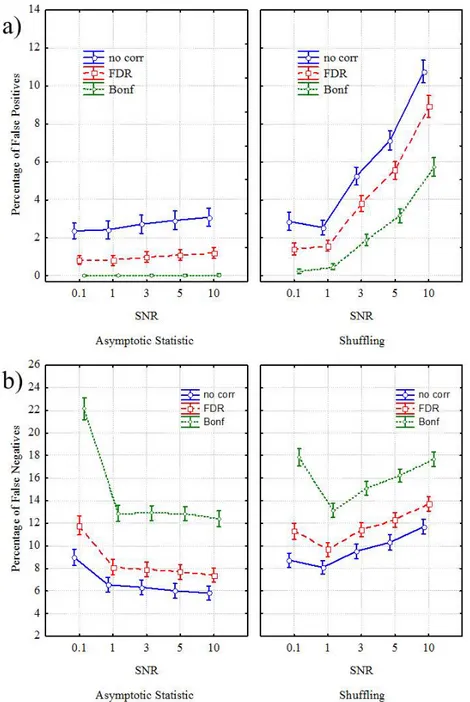
In Fig.1.4 I reported the results of ANOVA performed on the percentages of false positives (panel a) and false negatives (panel b) occurred during the validation procedure, using VALIDTYPE, SNR and CORRECTION as within main factors. The diagram shows the mean value of the two performance indexes achieved on connectivity patterns normalized according
31
to rows before the validation process, for different values of SNR and for different correction types (no correction in blue, FDR in red and Bonferroni in green) used for preventing type I errors in the statistical assessment procedure. The bar represented their relative 95% confidence interval.
Panel a highlighted statistical differences between the two validation methods in the occurrence of false positives across different SNR levels. The percentage of type I errors, achieved by applying Asymptotic Statistic procedure, for the SNR ranging from 0.1 to 10, increased from 2% to 4% for the no correction case, but remained constant around 1% for FDR case and 0.1% for Bonferroni adjustment. Post hoc analysis revealed statistical differences (p<0.00001) between all the SNR levels in the no correction case and with the exceptions of SNR 1 and 3 in FDR case, although this differences disappeared completely in Bonferroni case. The percentage of false positives, achieved by applying Shuffling procedure, was at 3% for SNR 0.1, decreased to 2% for SNR 1, then increased up to 11% for SNR 10 in the no correction case. The same trend but with lower percentages resulted for FDR and Bonferroni cases where the percentages increased up to 9% and 6% respectively along SNR levels. Duncan’s pairwise comparisons revealed statistical differences (p<0.00001) along all the levels of SNR for the three CORRECTION cases. The differences between the two validation types in the occurrence of false positives are statistical significant across all the SNR imposed and all the corrections applied, as stated by the Duncan’s pairwise comparisons.
Panel b showed statistical differences between the two validation types in the occurrence of type II errors across different SNR levels. In particular in the first diagram of panel b, for SNR values ranging from 0.1 to 1, the percentage of false negatives achieved applying Asymptotic Statistic procedure, decreased from 22% to 13% for the Bonferroni correction, from 12% to 8% for FDR adjustment and from 9% to 6% for no correction case. For SNR values ranging from 1 to 10 the percentages of type II errors remained constant around 13% for Bonferroni correction, 8% for FDR and 6% for no correction case. Duncan’s pairwise comparisons revealed statistical differences (p<0.00001) between all the SNR levels in all the three CORRECTION cases. In the second diagram of panel b, for SNR values ranging from 0.1 to 1, the percentage of false negatives reached applying Shuffling procedure, decreased from 18% to 13% for the Bonferroni correction, from 11% to 10% for FDR adjustment and from 9% to 8% for no correction case. For SNR values ranging from 1 to 10 the percentage of type II errors moved from 13% to 18% for Bonferroni correction, from 10% to 14% for FDR
32
and from 8% to 12% for no correction case. Pairwise comparisons revealed statistical differences (p<0.00001) between all the SNR levels in all the three CORRECTION cases. The differences between the two validation types in the occurrence of false negatives were statistical significant across all the SNR and all the corrections applied, as stated by the Duncan’s pairwise analysis.
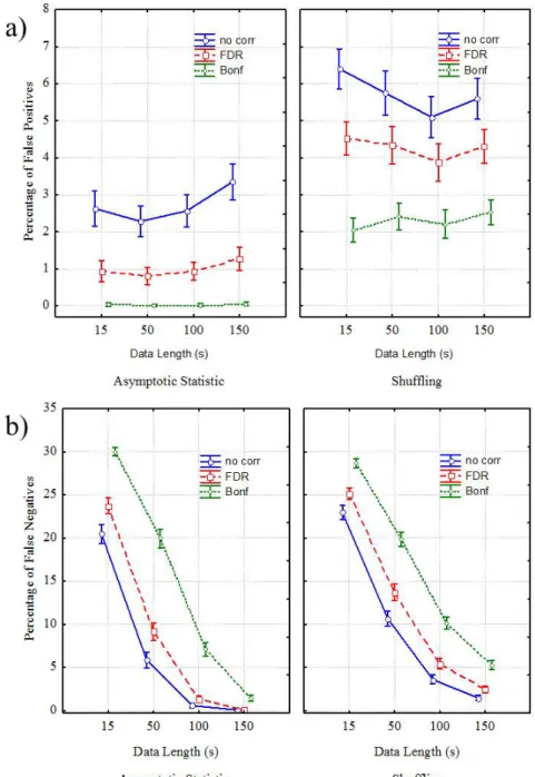
Figure 1.5 - Results of ANOVA performed on the percentages of false positives (a) and false negatives (b) occurred during the validation procedure, using VALIDTYPE, LENGTH and CORRECTION as within main factors. The diagram shows the mean value for the percentages, achieved by normalizing according to rows the inferred connectivity
patterns before the validation process, for different values of data length (in ms) and for different correction types (no correction in blue, FDR in red and Bonferroni in green). The bar represents their relative 95% confidence interval.
In Fig.1.5 I showed results of ANOVA performed on the percentages of false positives (panel a) and false negatives (panel b) occurred during the validation procedure, using
33
VALIDTYPE, LENGTH and CORRECTION as within main factors. The diagram shows the mean value for both indexes, achieved on connectivity patterns normalized according to rows before the validation process, for different values of data length (in ms) and for different correction types (no correction in blue, FDR in red and Bonferroni in green). The bar represented their relative 95% confidence interval.
Panel a highlighted statistical differences between the two validation methods in the occurrence of false positives across different data lengths. In fact, in the first diagram of panel a, the percentage of type I errors, achieved by applying Asymptotic Statistic procedure, for the data length ranging from 15s to 150s, increased from 2.5% to 3.5% for the no correction case, from 1% to 1.5% for FDR case but remained constant around 0.1% for Bonferroni adjustment. Post hoc analysis revealed statistical differences (p<0.00001) between all the different data lengths in the no correction case and with the exceptions of 50s and 100s in FDR case, although this differences disappeared completely in Bonferroni case. In the second diagram of panel a, the percentage of false positives, achieved by applying Shuffling procedure, for data length from 15s to 100s, moved from 6.5% to 5% for no correction case, from 4.5% to 4% for FDR case and remained around 2.5% for Bonferroni adjustment. For data length ranging from 100s to 150s, the percentages of false positives increased from 5% to 5.5% for no correction case, from 4% to 4.5% for FDR case and from 2 to 2.5% for Bonferroni adjustment. Duncan’s pairwise comparisons revealed statistical differences (p<0.00001) across all the different data lengths for all the three CORRECTION cases. The differences between the two validation types in the occurrence of false positives are statistical significant across all the data lengths and all the corrections applied, as stated by the Duncan’s test.
Panel b highligted statistical differences between the two validation methods in the occurrence of false negatives across different data lengths. In fact, in the first diagram of panel b, the percentage of type II errors, achieved by applying Asymptotic Statistic procedure, for the data length ranging from 15s to 150s, decreased from 30% to 2% for Bonferroni adjustment, from 25% to 1% for FDR, from 20% to 0% for the no CORRECTION case. Post hoc analysis revealed statistical differences (p<0.00001) between all the different data lengths in all the three correction cases. In the second diagram of panel b, the percentage of false negatives, achieved by applying Shuffling procedure, for data length from 15s to 150s, decreased from 28% to 5% for Bonferroni adjustment, from 25% to 2.5% for FDR case and from 23% to 2% for no correction case. Duncan’s analysis revealed statistical differences
34
(p<0.00001) across all the different data lengths for all the three CORRECTION cases. The differences between the two validation types in the occurrence of false negatives are statistical significant across all the data lengths and all the corrections applied, as stated by the Duncan’s pairwise comparisons.
In order to understand which type of links are responsible for the occurrence of type I errors, a new ANOVA was applied using the percentage of false positives as dependent variable and LINK, SNR and LENGTH as within main factors. I considered only the links corresponding to the imposed ‘null’ arcs because type I errors could occur only in their correspondence. A specific ANOVA was applied for each validation procedure and for each correction type. For the briefness of the text I reported only results achieved applying both Asymptotic Statistic and Shuffling methods and imposing a significance level FDR corrected, but the same conclusions can be inferred even for the other two correction cases. Results showed high statistical influence of the main factors LINK (P<0.00001, F=15.33) and LINK x SNR (P<0.00001, F=7.33) on percentage of false positives occurred during the Asymptotic Statistic procedure and high statistical influence of the main factors LINK (P<0.00001, F=2346), LINK x LENGTH (P<0.00001, F=16), LINK x SNR (P<0.00001, F=270) on percentage of false positives occurred during the Shuffling procedure.
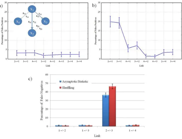
In Fig.1.6 I reported results of ANOVA performed on the percentage of false positives, occurred during the validation procedure computed by Asymptotic statistic (panel a) and Shuffling (panel b) methods, using LINK as within main factor. The diagram shows the mean value for the percentage achieved on each considered arc of the networks and its relative 95% confidence interval. Panel a showed the percentage of false positives, occurred during the Asymptotic Statistic procedure. In particular, such percentage was around 3.5% for links 2 → 1, 3 → 1 and 4 → 1 and around 2% for links 3 → 2, 4 → 2, 4 → 3, 2 → 4, 3 → 4. Duncan’s pairwise comparisons confirmed statistical differences (p<0.00001) between the links 2 → 1, 3 → 1 and 4 → 1 each other and with the other considered links.
35
Figure 1.6 – (a) and (b) Results of ANOVA performed on the percentage of false positives, occurred during the validation procedure computed through Asymptotic statistic (a) and Shuffling (b) methods, using LINK as within main
factor. I considered only the links corresponding to the imposed ‘null’ arcs because they can be origin of type I errors. The diagram shows the mean value for the percentage of false positives on each considered arc of the networks and their
relative 95% confidence interval. (c) The bar diagram shows the mean value, evaluated on different data lengths (in ms) and different SNR, for the percentages of type II errors, achieved by normalizing according to rows the inferred connectivity patterns before the validation process and validating them through Asymptotic statistic (blue columns) and
Shuffling (red columns) methods for a significance level of 5% FDR corrected.
Panel b showed a percentage of false positives, occurred during Shuffling validation process. In particular, such percentage was around 20% for links 2 → 1, 3 → 1, around 6% for link 4 → 1, around 7.5% for link 3 → 2 and from 1% to 4% for links 4 → 2, 4 → 3, 2 → 4, 3 → 4. Duncan’s analysis confirmed statistical differences (p<0.00001) between the links 2 → 1, 3 → 1, 4 → 1 and 3 → 2 each other and with the other considered links.
The bar diagram in Fig.1.6c showed the mean value, computed across different data lengths and SNR values, for the percentages of type II errors, achieved on connectivity patterns normalized according to rows before the validation process and validated through Asymptotic Statistic (blue columns) and Shuffling (red columns) for a significance level of 5% FDR corrected. The percentage of false negative is almost due to the link 2 → 3 whose imposed connection strength was really weak.