Measuring core inflation by multivariate structural time series models

MeasuringCoreInflation by Multivariate

Structural Time Series Models

Tommaso Proietti

CEIS Tor Vergata - Research Paper Series, Vol.

28, No. 83, May 2006

This paper can be downloaded without charge from the Social Science Research Network Electronic Paper Collection:

http://papers.ssrn.com

CEIS Tor Vergata

R

ESEARCH

P

APER

S

ERIES

Measuring Core Inflation by Multivariate

Structural Time Series Models

Tommaso Proietti1

Dipartimento S.E.F. e ME. Q. Universit`a di Roma “Tor Vergata”

1_{Address for Correspondence: Via Columbia 2, 00133, Rome. e-mail:}

tom-maso.proietti@uniroma2.it. This paper was prepared for the volume Optimisation, Econometric

and Financial Analysis, volume of the book series on ”Advances on Computational Management

Science”, Erricos John Kontoghiorghes and Cristian Gatu, Editors. The author wishes to thank Stephen Pollock and two anonymous referees for their very helpful suggestions.

Abstract

The measurement of core inflation can be carried out by optimal signal extraction tech-niques based on the multivariate local level model, by imposing suitable restrictions on its parameters. The various restrictions correspond to several specialisations of the model: the core inflation measure becomes the optimal estimate of the common trend in a mul-tivariate time series of inflation rates for a variety of goods and services, or it becomes a minimum variance linear combination of the inflation rates, or it represents the compo-nent generated by the common disturbances in a dynamic error compocompo-nent formulation of the multivariate local level model. Particular attention is given to the characterisation of the optimal weighting functions and to the design of signal extraction filters that can be viewed as two sided exponentially weighted moving averages applied to a cross-sectional average of individual inflation rates. An empirical application relative to U.S. monthly inflation rates for 8 expenditure categories is proposed.

Keywords: common trends, dynamic factor analysis, homogeneity, exponential smoothing, Wiener–Kolmogorov filter.

1

Introduction

Core inflation measures are considered to be more appropriate for the assessment of the trend movements in aggregate prices than is the official aggregate inflation rate. It is usually thought that the raw inflation rate, obtained as the percentage change in the consumer price index (CPI, henceforth) over a given horizon, is too noisy to provide a good indication of the inflationary pressures in the economy.

Like many other key concept in economics, there is no consensus on the notion of core inflation, despite the fact that quasi-official measures are routinely produced by statisti-cal agencies. This is because the notion serves a variety of purposes. Nevertheless, an increasing number of indices of core inflation are being produced in a variety of ways.

As a consequence, a large body of literature has been devoted to core inflation. An excellent review is Wynne (1999), who makes a basic distinction between methods which use only sectional information, and those which also use the time dimension. Another useful distinction is between aggregate or disaggregate approaches.

The most popular measures fall within the disaggregate approach, using only the cross-sectional distribution of inflation rates at a given point in time. They aim at reducing the influence of items that are presumed to be more volatile, such as food and energy. Other measures exclude mortgage interest costs, and some also exclude the changes in indirect taxes.

Bryan and Cecchetti (1994) (see also Bryan, Cecchetti and Wiggins II, 1997) argue that the systematic exclusion of specific items, such as food and energy, is arbitrary, and, after remarking that the distribution of relative price changes exhibits skewness and kurtosis, propose to use the median or the trimmed mean of the cross-sectional distribution.

Cross-sectional measures, using only contemporaneous price information, are not sub-ject to revision as new temporal observations become available, and this is often, although mistakenly, seen as an advantage. The corresponding core inflation measures tend to be rather rough and do not provide clear signals of the underlying inflation. We show here that measures that are constructed via a time series approach are better behaved.

Other approaches arise in the structural vector autoregressive (VAR) framework, start-ing from the seminal work of Quah and Vahey (1995), who, within a bivariate stationary VAR model of real output growth and inflation, defined core inflation as that component of measured inflation which has no long run effect on real output.

This paper considers the measurement of core inflation in an unobserved components framework; in particular, the focus will be on dynamic models that take a stochastic approach to the measurement of inflation, such as those introduced in Selvanathan and Prasada Rao (1994, ch. 4). We propose and illustrate measures of core inflation that arise when standard signal extraction principles are applied to restricted versions of a workhorse model, which is the multivariate local level model (MLLM, henceforth).

The parametric restrictions are introduced in order to accommodate several important cases: the first is when the core inflation measure is the optimal estimate of the common trend in a multivariate time series of inflation rates for a variety of goods and services. In an alternative formulation it is provided by the minimum variance linear combination of the inflation rates. In another it arises as the component generated by the common

disturbances in a dynamic error component formulation of the MLLM.

Particular attention is devoted to the characterisation of the Wiener–Kolmogorov op-timal weighting functions and to the design of signal extraction filters that can be viewed as a two sided exponentially weighted moving averages applied to a contemporaneously aggregated inflation series.

The paper is organised as follows. Section 2 deals with aggregate measures of core inflation and their limitations. The MLLM and its main characteristics are presented in section 3. Signal extraction for the unrestricted MLLM is considered in section 4. Section 5 introduces several measures of core inflation that can be derived from the MLLM under suitable restrictions of its parameters. In particular, we entertain three classes of restric-tions, namely the common trend, the homogeneity, and the dynamic error components restrictions. Section 6 derives the signal extraction filters for the dynamic factor model proposed by Bryan and Cecchetti (1994); and it compares them with those derived from the MLLM. Inference and testing for the MLLM and its restricted versions are the topic of section 7). Finally, in section 8, the measures considered in the paper are illustrated with reference to a set of U.S. time series concerning the monthly inflation rates for 8 expenditure categories.

2

Aggregate measure of core inflation

Statistical agencies publish regularly two basic descriptive measures of inflation that are built upon a consumer or retail price index. The first is the percentage change over the previous month. The second is the percent change with respect to the same month of the previous year.

Unfortunately, neither index is a satisfactory measure of trend inflation. The first turns out to be very volatile, as it is illustrated by the upper panel of figure 1, which displays the monthly inflation rates for the for U.S. consumer price index (city average, source: Bureau of Labor Statistics) for the sample period 1993.1-2003.8. By contrast, the annual changes in relative prices are much smoother (see the lower panel of figure 1), but, being based on an asymmetric filter, they suffer from a phase shift in the signal, which affects the timing of the turning points in inflation. Furthermore, if the consumer price index is strictly non seasonal, then the series of yearly inflation rates is non invertible at the seasonal frequencies. With pt representing the price index series, and with yt = ln(pt/pt−1), the

yearly inflation rate is approximately S(L)y_t, where S(L) = 1 + L + L2_{+ · · · + L}11_{, which} is a one sided filter with zeros at the seasonal frequencies.

One approach, which is followed by statistical agencies, is to reduce the volatility of inflation by discarding the goods or services that are presumed to be more volatile, such as food and energy. The monthly and yearly inflation rates constructed from the CPI excluding Food and Energy are indeed characterised by reduced variability, as figure 1 shows; yet they are far from satisfactory and they can be criticised on several grounds, not the least of which is their lack of smoothness.

1993 1994 1995 1996 1997 1998 1999 2000 2001 2002 2003 −0.25

0.00 0.25 0.50

Monthly inflation rates CPI ExFood&Energy

1993 1994 1995 1996 1997 1998 1999 2000 2001 2002 2003 2

3

Yearly inflation rates

CPI ExFood&Energy

Figure 1: U.S. CPI Total and Excluding Food & Energy, 1993.1-2003.8. Monthly and yearly inflation rates.

3

The multivariate local level model

The measures of core inflation proposed in this paper arise from applying optimal signal extraction techniques derived from various restricted versions of a multivariate times series model. The model in question is the multivariate generalisation of the local level model (MLLM), according to which a multivariate time series can be decomposed into a trend component, represented by a multivariate random walk, and a white noise (WN) compo-nent. Letting yt denote an N × 1 vector time series referring to the monthly changes in

the prices of N consumer goods and services,

yt = µt+ ²t, t = 1, 2, . . . , T, ²t∼ WN(0, Σ²),

µ_t = µ_t−1+ η_t, η_t∼ WN(0, Ση). (1)

The disturbances η_tand ²_tare assumed to be mutually uncorrelated and uncorrelated to µ₀.

Before considering restricted versions of the model, we review its main features both in the time and the frequency domain (see Harvey, 1989, for more details). The model assumes that the monthly inflation rates are integrated of order one (prices are integrated of order two). This assumption can actually be tested. In section 7 we review the locally best invariant test of the hypothesis that monthly inflation rates are stationary versus the alternative that they are I(1). Taking first differences, we can reexpress model (1) in its stationary form:

∆y_t= η_t+ ∆²_t.

The crosscovariance matrices of ∆yt, Γ∆(τ ) = E(∆yt∆y0t−τ) are then

Γ∆(0) = Ση+ 2Σ²,

Γ_∆(1) = Γ_∆(−1)0 _{= −Σ} ²,

Γ∆(τ ) = 0, |τ | > 1.

Notice that the autocovariance at lag 1 is negative (semi)definite and symmetric: Γ∆(1) = Γ∆(1)0 = Γ∆(−1). This symmetry property implies that the multivariate spec-trum is real-valued. Denoting by F(λ) the spectral density of ∆y_t at the frequency λ, we have F(λ) = (2π)−1[Ση+ 2(1 − cos λ)Σ²]. The autocovariance generating function

(ACGF) of ∆yt is

G(L) = Ση+ |1 − L|2Σ². (2)

The reduced form of the MLLM is a multivariate IMA(1,1) model: ∆y_t= ξ_t+ Θξ_t−1.

Equating (2) to the ACGF of the vector MA(1) representation for ∆yt, it is possible to

show that the parameterisation (1) is related to the reduced form parameters via: Σ_η = (I + Θ)Σ_ξ(I + Θ0), Σ_ε = −ΘΣ_ξ= −Σ_ξΘ0.

The structural form has N (N + 1) parameters, whereas the unrestricted vector IMA(1,1) model has N2 _{+ N (N + 1)/2. In fact, Σ}

ε = −ΘΣξ = −ΣξΘ0 imposes N (N − 1)/2

4

Signal extraction

Assuming a doubly infinite sample, the minimum mean square linear estimator (MMSLE) of the underlying level component is

˜

µ_t= W(L)y_t, with weighting matrix polynomial

W(L) = |1 − L|2Gµ(L)G(L)−1 = Ση

¡

Ση+ |1 − L|2Σ²

¢₋₁ ,

where Gµ(L) is the pseudo ACGF of the trend component and we have defined |1 −

L|2 _{= (1 − L)(1 − L}−1_{). This results from the application of the Wiener–Kolmogorov}

(WK, henceforth) filtering formulae given in Whittle (1983), which apply also to the nonstationary case (Bell, 1984).

The matrix polynomial W(L) performs two-sided exponential smoothing W(L) = (I + Θ)Σξ(I + Θ0)(I + Θ0L−1)−1Σ−1_ξ (I + ΘL)−1

and it has W(1) = I_N, which generalises to the multivariate case the unit sum property of the weights for the extraction of the trend component.

The filtered or real time estimator of the trend is an exponentially weighted average of current and past observations:

˜

µ_t|t = (I + Θ)(I + ΘL)−1yt

= (I + Θ)P∞_j=0(−Θ)j_y t−j.

5

Measures of core inflation derived from the MLLM

In this section we explore that have to be imposed on the WK filter to make it yield univariate summary measures of tendency of the form:

˜

µt= w(L)0yt, w(L) = q(L)w (3)

where q(L) is a univariate symmetric two-sided filter and w is a static vector of cross-sectional weights. Purely static measures arise when q(L) = 1. The signal extraction filters of (3) are the basis of the measurement of core inflation, when yt represents N

inflation rates that have to be combined in a single measure.

The cross-sectional weights can be model based or they can originate from a priori knowledge. It is instructive to look at the various ways that they can originate and at their different various meanings.

5.1 Aggregate measures (known weights)

The first core inflation measures arise from the contemporaneous aggregation of the mul-tivariate trend component in (1) using known weights. The MLLM is invariant under

contemporaneous aggregation; thus, w0_y

t, where w is a vector of known weights (e.g.

expenditure shares in the core inflation example), follows a univariate local level model. The aggregated time series, w0_y

t, has thus a local level model representation, and the

miminum-mean-square linear estimator of the trend component, w0_µ

t, based on a doubly

infinite sample, has the above structure (3), with:

q(L) = 1 1 + q−1_{|1 − L|}2 = (1 + θ)2 |1 + θL|2 (4) and q = w0_Σ ηw/w0Σ²w, and θ = [ p (q2_{+ 4q − 2 − q]/2, −1 < θ ≤ 0.}

Alternatively, we could fit a univariate local level model to the aggregate time series. The corresponding core inflation measure is given by (4), but q would be estimated directly, rather than obtained from the aggregation of the covariance matrix of the disturbances of the multivariate specification.

5.2 Common trend

Common trends arise when rank(Ση) = K < N , so that

Ση = ZΣη†Z0

where Z is N × K and Σ_η† is a full rank K × K matrix.

When there is a single common trend, K = 1, driving the µ_t’s in (1), we can write: yt= zµt+ µ0+ ²t,

where z is a N × 1 vector of loadings and µt= µt−1+ ηt, ηt∼ WN(0, ση2).

The WK filter for µt, assuming a doubly infinite sample, takes the form (3) with

w = (z0Σ−1_² z)−1Σ−1_² z, (5)

and q(L) given by (4), where the signal–noise ratio is given by q = σ_η2(z0Σ−1_² z).

If Σ² is diagonal (i.e. if it represents the idiosyncratic noise) and z is a constant vector

(the common trend enters the series with the same coefficient) then the cross-sectional weights (5) applied to ytproduce a weighted average ¯yt= w0yt, in which the more noisy

series are downweighted. The application of the univariate two sided filter q(L), which is a bidirectional exponentially weighted average, to ¯yt yields the estimated component.

The expression (5) assumes that Σ² is full rank; if its rank is N − 1 then q(L) = 1

and w = (v0_z)−1_{v, where v is the eigenvector corresponding to the zero eigenvalue of Σ} ².

5.3 Homogeneity

The MLLM is said to be homogeneous if the covariance matrices of the disturbances are proportional (see Enns et al., 1982, and Harvey, 1989, ch. 8):

Ση = qΣ².

Here, q denotes the proportionality factor.

Under homogeneity, the model is a seemingly unrelated IMA(1,1) process ∆yt= ξt+

θξ_t−1, with scalar MA parameter, θ = [p(q2_{+ 4q − 2 − q]/2, taking values in [-1,0], and}

ξ_t∼ WN(0, Σξ), Σξ= −Σ²/θ.

The trend extraction filter is scalar and can be applied to each series in turn: ˜

µ_t= 1

1 + q−1_{|1 − L|}2yt.

As a matter of fact, the Kalman filter and smoother become decoupled, and inferences are particularly simplified (see also section 7).

Consider forming a linear combination of the trend component µ_t: ¯µt = w0µt.

Obvi-ously,

˜¯µ_t|∞= 1

1 + q−1_{|1 − L|}2w0yt.

If w is known (as in the case of expenditure shares), then the summary measure coincides with that arising from the aggregate approach. The difference, however, lies with the signal–noise ratio, which is estimated more efficiently if the model is homogeneous. Again, the measure of core inflation is a static weighted average, with given weights, of the individual trends characterising each of the series.

Consider now the alternative strategy of forming a measure of the type (3) by means of a static linear combination of the estimated trends, ˜µt= w0µ˜t, with weights

w = Σ −1 η z z0_Σ−1 η z . (6)

It is easy to show that the weights w produce the linear combination w0_µ

twhich minimises

the variance w0Σηw under the constraint w0z = 1, where z is an arbitrary vector. Hence,

these weights provide the smoothest (i.e. the least variable) component that preserves the level (w0_{i = 1), where i is an N × 1 vector with unit elements, i = [1, . . . , 1]}0_.

Another interpretation of (6) is that w0µ_t is the GLS estimates of µt in the model

µ_t = zµt+ µ∗t, considered as a fixed effect; w0yt are known as Bartlett scores in factor

analysis (see Anderson, 1984, p. 575). Notice, however, that here z is a known vector, that has to be specified a priori (e.g. we may look for weights summing up to unity, in which circumstance, z = i). It is not a necessary feature of the true model.

5.4 Dynamic error components

Suppose that the level disturbances have the following error components structure (Mar-shall, 1992):

where ηt is disturbance that is common to all the trends and η∗t is the idiosyncratic

disturbance (typically, but not necessarily, Nη is a diagonal matrix). Correspondingly,

Σ_η = σ2

ηzz0+ Nη, and the trends can be rewritten as

µt= zµt+ µ∗t, ∆µt= ηt, ∆µ∗t = η∗t.

In general, the WK filter for µt does not admit the representation (3), as we have:

˜ µ_t= σ 2 η 1 + σ2 ηz0A(L)−1z z0A(L)−1y_t, A(L) = N_η+ |1 − L|2Σ_². However, if Nη = q∗Σ², then the WK filter takes the form (3) with

q(L) = σ 2 ηz0N−1η z σ2 ηz0N−1η z + 1 + q−1|1 − L|2 (7) and w = N −1 η z z0_N−1 η z = Σ −1 ² z z0_Σ−1 ² z .

This type of homogeneity may arise, for instance, when the idiosyncratic trend distur-bances are a fraction of the irregular component, that is η∗

t = ρ²t, ρ2 = q∗. This makes

the overall trend and irregular components correlated, but µt would still be uncorrelated

with ²_t.

Now let us consider the case when ²t has the same error components structure: ²t =

z²t+ ²∗t, with ²t∼ WN(0, σ2²), ²∗t ∼ WN(0, N²), so that

Σ²= σ2²zz0+ N².

The WK filter for µt is now

˜ µt= σ2 η 1 + σ2 ηz0A(L)−1∗z z0A(L)−1∗yt, A(L)∗= Nη + |1 − L|2N²,

and, under the homogeneity condition Nη = q∗N², produces exactly the same filter as the

previous case, with q∗ _{replacing q in (7).}

Gathering the components driven by the common disturbances into ςt = µt+ ²t, and

writing yt= zςt+ µ∗t + ²∗t, the MMSLE of ςt is

˜

ς_t= c(L)

1 + c(L)z0_A(L)−1∗_zz

0_A(L)−1∗_y

t, c(L) = ση2(1 + q−1|1 − L|2), q = σ2η/σ²2.

Moreover, if N_η = qN_², with the same q, σ2

ηA(L) = c(L)Nη, then ˜ςt is extracted by a

static linear combination with weights

w = N

−1 η z

ση−2+ z0N−1η z

Notice that this last case arises when the system is homogeneous Ση = qΣ², and Σ² has

an error component structure. Otherwise, if Nη = ση2∗I, N_²= σ2_²∗I, then the filter for ς_t is

as in (3) with w = z and q(L) = σ 2 η(1 + q−1|1 − L|2) σ2 η∗(1 + q−1∗|1 − L|2) , q∗= σ_η∗2 /σ_²2∗

6

Dynamic factor models

This section discusses the signal extraction filters that are optimal for a class of dynamic factor models proposed by Stock and Watson (1991) for the purpose of constructing a model-based index of coincident indicators for the U.S. econonomy.

This class has been adopted by Bryan and Cecchetti (1994) for the measurement of core inflation, and it applies to a vector of monthly inflation rates, yt, which are expressed

as as follows: yt = zµt+ µ∗t, ϕ(L)µt = ηt, ηt∼ WN(0, σ2η) D(L)µ∗ t = η∗t, η∗t ∼ WN(0, Nη) (8) where D(L) = diag{di(L), i = 1, . . . , N }, and ϕ(L) and di(L) are AR scalar polynomials,

possibly nonstationary, Nη = diag{σ2i∗, i = 1, . . . , N }, and ηt is uncorrelated with η∗t at

all leads and lags.

The autocovariance generating function of µtand the cross-covariance generating

func-tion of y_t are respectively: gµ(L) =

σ2

η

|ϕ(L)|2, Γy(L) = gµ(L)zz0+ M(L), where we have written

M(L) = D(L)−1NηD(L−1)−1 = diag{σ2i∗|di(L)|−2, i = 1, . . . , N }.

Moreover, the cross-covariance generating function between µt and yt is simply gµ(L)z0.

Hence, the WK signal extraction formula is: ˜ µ_t = g_µ(L)z0_[Γ y(L)]−1yt = £gµ(L)−1+ z0M(L)−1z ¤₋₁ z0_M(L)−1_y t = £σ−2 η |ϕ(L)|2+ P i|di(L)|2σi∗−2 ¤₋₁P_N i=1|di(L)|2σ−2i∗ yit.

When ϕ(L) = d_i(L), i = 1, . . . , N, which is a seemingly unrelated time series equations (SUTSE) system, the WK specialises as follows:

˜ µt= " σ_η−2+ N X i=1 1 σ2 i∗ #_{−1 N} X i=1 1 σ2 i∗ yit= [ση−2+ z0N−1η z]−1z0N−1η yt.

Hence, ˜µ_tresults only from the contemporaneous aggregation of the individual time series, with weights that do not sum to unity, although they are still proportional to the reciprocal of the specific variances. If ϕ(L) = ∆, then the dynamic factor model (8) is a special case of the MLLM (1), with no irregular component.

7

Inference and testing

The state space methodology provides a means of computing the minimum-mean-square linear estimators (MMSLE) of the core inflation component, µt, and of any latent variable

in the model. In finite samples the MMSLE of µ_tin (1) is computed by Kalman filter and the associated smoothing algorithm (see Durbin and Koopman, 2001).

The Kalman filter (KF) is started off at t = 2 with ˜µ_2|1 = y1 and P2|1 = Σ² + Ση

computes for t = 2, . . . , T :

νt= yt− ˜µt|t−1, Ft= Pt|t−1+ Σ²

Kt= Pt|t−1F−1t ,

˜

µ_t+1|t= ˜µ_t|t−1+ Ktνt, Pt+1|t= Pt|t−1+ Ση− KtFtK0t.

Denoting the information up to time t by Yt = {y1, y2, . . . , yt}, the above quantities

have the following interpretation: νt = yt− E(yt|Yt−1), Ft = Var(yt|Yt−1), ˜µt|t−1 =

E(µ_t|Yt−1), Pt|t−1 = Var(µt|Yt−1) ˜µt= E(µt|Yt), Pt= Var(µt|Yt).

The Kalman filter performs the prediction error decomposition of the likelihood func-tion. The latter can be maximised using a quasi-Newton numerical optimisation method. When the model is homogeneous, inferences are made easier by the fact that the Kalman filter and smoother become decoupled. In fact, at t = 2, ˜µ_2|1= y₁ and P_2|1= (q + 2)Σ_²= p_2|1Σ², where we have written p2|1 = (q + 1). Now, consider the KF quantities that are independent of the data:

Ft = Pt|t−1+ Σ², Kt= Pt|t−1F−1t ,

P_t+1|t = P_t|t−1+ qΣ²− Pt|t−1F−1t Pt|t−1;

F_t and P_t+1|t will be proportional to Σ_²: F_t = f_tΣ_², P_t|t−1 = p_t|t−1Σ_²; also, K_t = p_t|t−1/(1 + p_t|t−1)IN, where the scalar quantities are delivered by the univariate KF for

the LLM with signal to noise ratio q.

Hence, the innovations and inferences about the states can be from N univariate KFs. Correspondingly, it can be shown that Σ²can be concentrated out the likelihood function,

and the concentrated likelihood can be maximised with respect to q (see Harvey, 1989, p. 439).

7.1 Homogeneity tests

The Lagrange multiplier test of the homogeneity restriction, H0 : Ση = qΣ², was derived

in the frequency domain by Fernandez and Harvey (1970). The frequency domain log-likelihood function is built on the stationary representation of the local level model, ∆y_t= η_t+ ∆²tand it takes the form:

L(ψ) = −N T∗ 2 ln 2π − 1 2 T∗₋₁ X j=0 n ln |Gj| + 2π · trace h G−1_j I∗(λj) io ,

where T∗ _{= T − 1, ψ is a vector containing the p = N (N + 1) unknown parameters of}

λj = 2πj/T∗, Gj = Ση+ 2(1 − cos λj)Σ² is the spectral generating function of the MLLM

evaluated at the Fourier frequency λj and I∗(λj) is the (real part of) multivariate sample

spectrum at the same frequency.

The LM test of the restriction H0: ψ = ψ0 takes the form

LM = DL(ψ₀)I(ψ₀)−1DL(ψ₀)0 (9) where DL(ψ₀) is 1 × p vector containing the partial derivatives with respect to the pa-rameters evaluated at the null and I(ψ₀) is the information matrix evaluated at ψ₀. Expressions for DL(ψ₀) and I(ψ₀) are given in Fernandez and Harvey (1990).

The unrestricted local level model has N (N + 1) parameters, whereas the homogenous model has N (N + 1)/2 + 1, so the test statistic (9) is asymptotically distributed as a χ2 random variable with N (N + 1)/2 − 1 degrees of freedom.

The homogeneous dynamic error component model further restricts Σ² = σ¯²ii0+ N²,

and when the disturbances ²∗

t are fully idiosyncratic, the model has only N +2 parameters.

This restriction can be tested using (9), which gives a χ2 _{test with N (N + 1) − N − 2} degrees of freedom.

7.2 Testing for a multivariate RW and for common trends

Nyblom and Harvey (2000, NH henceforth) have developed the locally best invariant test of the hypothesis H0 : Ση = 0 against the homogenous alternative H1 : Ση = qΣ². The

test statistic is ξN = tr[ˆΓ−1S], where S = 1 T2 T X t=1 " t X i=1 (y_i− ¯y)(y_i− ¯y)0 # ˆ Γ = 1 T T X t=1 (yt− ¯y)(yt− ¯y)0

and has rejection region ξ_N > c. Under the null hypothesis, the limiting distribution of ξ_N is Cram`er-von Mises with N degrees of freedom. Although the test maximises the power against a homogeneous alternative, it is consistent for any Ση.

A non parametric adjustment, along the lines of the KPSS test, is required when ²_t is serially correlated and heteroscedastic. This is obtained by replacing ˆΓ with

ˆ Γl= ˆΓ(0) + l X τ =1 µ 1 − τ l + 1 ¶ [ˆΓ(τ ) + ˆΓ(τ )0] where ˆΓ(τ ) is the autocovariance of ytat lag τ .

When the test is applied to the linear transformation A0_y

t, where A is a known r ×

N matrix, testing the stationarity of A0yt amounts to testing the null that there are r

cointegrating relationships. If A0_Σ

ηA = 0, then we can rewrite yt= Zµt+ µ0+ ²t, with

A0_{Z = 0, so that A}0_y

The test statistics for this hypothesis is

ξr(A) = tr[(A0ΓA)ˆ −1A0SA],

and its limiting distribution is Cram`er-von Mises with r degrees of freedom.

NH also consider the test of the null hypothesis that there are k common trends, versus the alternative that there are more.

H0: rank(Ση) = k, vs. H1: rank(Ση) > k.

The test statistic is based on the sum of the N − k smallest eigenvalues of ˆΓ−1S, ζ(k, N ) = λk+1+ . . . + λN

The significance points of ζ(k, N ) are tabulated in NH (2000) for a set of (k, N ) pairs.

8

Illustration

Our illustrative example deals with extracting a measure of core inflation from a multi-variate time series consisting of the monthly inflation rates for 8 expenditure categories.

The series are listed in table 1 and refer to the U.S. city average for the sample pe-riod 1993.1-2003.8 (source: Bureau of Labor Statistics). The relative importance of the components of the U.S, inflation rate in building up the U.S. inflation rate, i.e. their CPI weights, is reported in the second column of table 3. Figure 2 displays the eight series yit, i = 1, 2, . . . , 8.

Table 1: Description of the series and their CPI weights.

Expenditure group CPI weights

1. Food and beverages 0.162

2. Housing 0.400

3. Apparel 0.045

4. Transportation 0.176

5. Medical care 0.058

6. Recreation 0.059

7. Education and communication 0.053 8. Other goods and services 0.048

Fitting the univariate local level model to w0yt, where w is the vector containing

the CPI weights reproduced in the second column of table 3, that is w0_y

t = µt+ ²t, ²t∼

WN(0, σ2

²), µt= µt−1+ηt, ηt∼ WN(0, qσ²2), gives the maximum likelihood estimate ˜q = 0.

The estimated signal to noise ratio implies that CPI monthly inflation is stationary and that the corresponding aggregate core inflation measure is represented by the time average of the CPI all items monthly inflation rates, that is ˜µ = T−1P

1995 2000 0.0000 0.0025 0.0050 0.0075 0.0100 DLFood&Beverages DLHousing 1995 2000 −0.02 −0.01 0.00 0.01 0.02 DLApparel DLTransportation 1995 2000 −0.0025 0.0000 0.0025 0.0050 0.0075 DLMedicalCare DLRecreation 1995 2000 0.00 0.01 0.02 0.03 0.04 DLEducation&Communication DLOtherGoods&Services

Figure 2: U.S. CPI, 1993.1-2003.8. Monthly relative price changes for the eight expendi-ture categories.

8.1 Stationarity and common trends

The issue concerning the stationarity of CPI monthly inflation can be also be handled within a multivariate framework. Assuming that yt= (y1t, . . . , y8t)0 is modelled as in (1), we can use the NH statistic ξ_N to test H₀ : Σ_η = 0 versus the alternative that Σ_η = qΣ_². The values of the NH statistic are reported in the second column of table 2 for various values of the truncation lag l used in computing the Newey-West nonparametric correc-tion for autocorrelacorrec-tion and heteroscedasticity. They lead to reject the null that y_t is stationarity for values of l up to 5.

Table 2: Nyblom and Harvey (2000) stationarity test, cointegration test and common trend test.

Truncation lag (l) NH NH-coint CT(1) 0 3.334 2.510 1.112 1 2.876 2.306 0.982 2 2.638 2.134 0.894 5 2.214 1.787 0.720 10 1.682 1.346 0.605 5% crit. value 2.116 1.903 0.637

The third column reports the values of the NH-cointegration test. The latter tests the null hypothesis that A0_y

t is stationary, where A is chosen such that A0i = 0, which

corresponds to the hypothesis that there is a single common trend which enters each of the series with the same loading; this is also known as the balanced growth hypothesis: as the series share the same common trend, the difference between any pair is stationary. This hypothesis is clearly rejected for low values of the truncation parameter, up to l = 2. Finally, CT(1) is the statistic for testing the null hypothesis that a single common trend is present (the 5% critical value has been obtained by simulation), based on the statistic ζ(1, 8) =P8_i=2λi(S−1C), where λi(·) is the i-th ordered eigenvalue of the matrix

in argument.

Taken together, the results of the NH-coint and CT(1) tests do not suggest the presence of a single common trend driving the eight CPI monthly inflation rates. Nevertheless, if the MLLM is estimated with a single common trend (see section 5.2) then the estimated vector of loadings is

˜z0= [1.000, 0.038, 0.069, 0.081, 0.016, 0.086, 0.023, −0.021], and the estimated trend disturbance variance is ˜σ2

η = 0.00065282. Estimation of the

MLLM with common trends was carried out in Stamp 6 by Koopman et al. (2000). The other computations and inferences were performed in Ox 3 by Doornik (2001). It can be seen that the series Food and beverages plays a dominant role in the definition of the common trend.

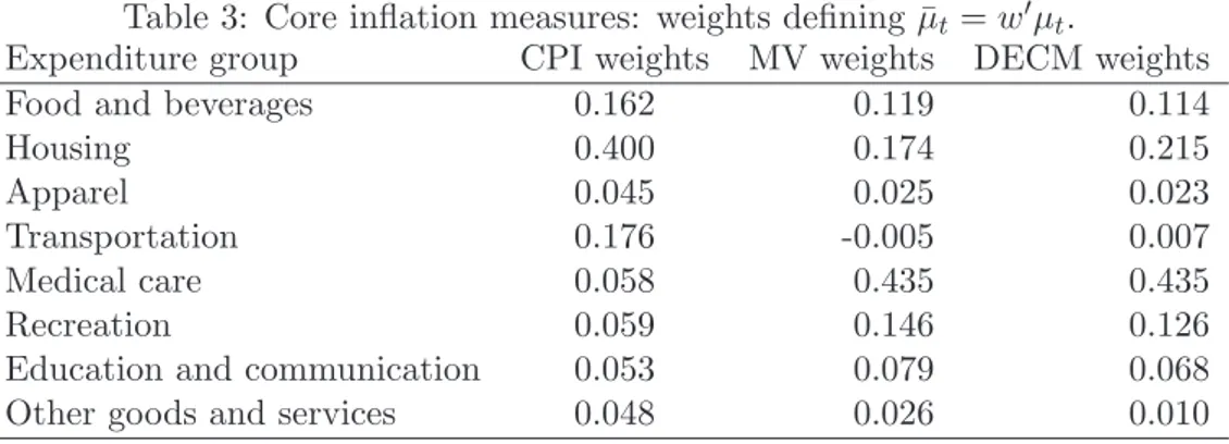
Table 3: Core inflation measures: weights defining ¯µt= w0µt.

Expenditure group CPI weights MV weights DECM weights

Food and beverages 0.162 0.119 0.114

Housing 0.400 0.174 0.215

Apparel 0.045 0.025 0.023

Transportation 0.176 -0.005 0.007

Medical care 0.058 0.435 0.435

Recreation 0.059 0.146 0.126

Education and communication 0.053 0.079 0.068

Other goods and services 0.048 0.026 0.010

8.2 Homogeneous MLLM

Maximum likelihood estimation of the local level model (1) with the homogeneity restric-tion is particularly straightforward, since the innovarestric-tions and inferences about the states can be obtained by running N univariate Kalman filters (this is known as decoupling). The matrix Σ²can be concentrated out the likelihood function and the concentrated likelihood

can be maximised with respect to the signal-noise ratio q. The estimation results are the following: ˆq = 0.0046, and

˜ Σ² =             0.04 −0.10 0.04 0.07 0.02 −0.04 −0.03 −0.01 −0.00 0.02 0.04 0.23 0.05 0.13 0.07 −0.10 0.00 0.00 0.17 0.07 −0.01 −0.00 −0.08 −0.08 0.01 0.02 0.02 0.55 0.04 0.10 −0.22 0.02 0.00 0.00 −0.00 0.00 0.01 −0.14 −0.02 −0.07 −0.00 0.00 −0.00 0.01 −0.00 0.03 −0.06 −0.04 −0.00 0.00 −0.01 −0.04 −0.00 −0.00 0.06 −0.14 −0.00 −0.01 −0.02 0.01 −0.00 −0.00 −0.02 0.39            

where in the upper triangle we report the correlations, which are usually very low. The frequency domain test for homogeneity (Fernandez and Harvey, 1990) takes the value 31.275 on 35 degrees of freedom and therefore it is not significant (the p-value is 0.65). This suggests that the homogenous specification is a good starting point for building up core inflation measures.

8.3 Homogeneous Dynamic Error Components model

Within the homogeneous model of the previous subsection we considered the error com-ponent structure Σ² = σ2²ii0+ N², in which there is a common disturbance linking the

trends and the irregular component; N² was specified as a diagonal matrix.

When estimated by maximum likelihood, the signal–noise ratio is close to that of the homogenous case, ˆq = 0.0043; moreover, the common irregular disturbance variance is estimated ˆσ2

¯

² = ×10−7 and

ˆ

However, the DECM restriction, H0 : Σ² = σ¯²2ii0 + N², Ση = qΣ², is strongly rejected,

with the LM test taking the value 153.43 on 60 degrees of freedom.

8.4 Core inflation measures

Bearing in mind the empirical results of the previous sections, we now discuss three mea-sures of core inflation obtained from the multivariate MLLM.

The first is derived from the homogeneous local level model and is defined as w0_µ˜ t|T,

where ˜µ_t|T are the smoothed estimates of the trends and w is the vector of CPI weights, equal to the budget share of the expenditure groups. This is reproduced along with the 95% confidence interval in the first panel of figure 3.

The second measure uses the minimum variance (MV) weights w = ˆΣ−1

² i/(i0Σˆ−1² i),

reproduced in the third column of table 3. Housing and Transportation result heavily downweighted (the MV weight is negative for the latter). The corresponding core inflation measure, displayed in the right upper panel of figure 3, is much smoother than the previous, and characterised by lower estimation error variance.

The last measure of core inflation is derived from the dynamic error component local level model with homogeneity and is defined as w0_µ˜

t|T, where w = N−1η i/(i0N−1η i) where

N_ηis a diagonal matrix. Although the DECM restriction was strongly rejected, the weights and the corresponding core inflation measure agree very closely with the minimum variance one.

The overall conclusion is that the point estimates of the three core inflation measures agree very closely.

For comparison purposes, in the last panel of figure 3 we display the core inflation measure estimated using the structural VAR approach by Quah and Vahey (1995, QV henceforth). A bivariate vector autoregressive (VAR) model was estimated for the series ut= [∆yt, ∆xt]0,

Φ(L)ut= β + ξt, Φ(L) = I − Φ1L − · · · − ΦpLp,

where yt is the monthly inflation rate, computed using the CPI total, and xt is the

loga-rithm of the industrial production index (source: Federal Reserve Board, sample period: 1993.1-2003.8). The VAR lag length which minimises the Akaike information criterion resulted p = 11, which is close to the value adopted by QV in their original paper. QV define core inflation as the component of inflation that can be attributed to nominal distur-bances that have no long run impact on output. Their identification proceeds as follows: the structural disturbances, ζ_t = [ζ1t, ζ2t]0, are defined as linear transformations of the time series innovations, ξt = Bζt, where B = {bij; i, j = 1, 2} is a full rank matrix such

that Φ(1)−1_{B is upper triangular (i.e. the nominal disturbance ζ}

1t has no permanent effect on xt). Correspondingly, the core inflation measure is:

mt= [ϕ11(L)b11+ ϕ12(L)b21]ζ1t, where Φ(L)−1 = {ϕij(L); i, j = 1, 2}.

Several differences arise with the measures extracted from the MLLM. The QV measure tracks actual inflation very closely; this lack of smoothness can be partly attributed to

1995 2000 −0.25

0.00 0.25 0.50

Homogeneous model, CPI weights

Inflation Core Inflation

1995 2000

−0.25 0.00 0.25 0.50

Homogeneous model, minimum variance weights

Inflation Core Inflation

1995 2000

−0.25 0.00 0.25 0.50

Dynamic Error Component Model

Inflation Core Inflation

1995 2000

−0.25 0.00 0.25 0.50

0.75 Structural VAR (Quah and Vahey, 1995) Inflation Core Inflation

Figure 3: U.S. CPI, 1993.1-2000.12. Core inflation measures derived from a multivariate local level model with homogeneity and variance components restrictions.

the fact that this measure is based on a one sided filter. The plot clearly show that mt is

indeed very volatile.

9

Conclusions

The paper has illustrated how core inflation measures can be derived from optimal signal extraction principles based on the multivariate local level model. The approach is purely statistical, in that a coherent statistical representation of the dynamic features of the series the model is sought, along with sensible ways of synthesizing the dynamics of a multivariate time series in a single indicator of underlying inflation. The advantage over indices excluding particular items, such as food and energy, is that maximum likelihood estimation of the parameters of the model indicate what items have to be downweighted in the estimation of core inflation.

Two main directions for future research can be envisaged: the first is enlarging the cross-sectional dimension by using more disaggregate price data. The second is to provide more economic content to the measurement by including in the model a Phillips’ type relationship featuring among the inflation determinants measures of monetary growth, the output gap and inflation expectations.

References

Anderson, T.W. (1984), An Introduction to Multivariate Statistical Analysis, Second Edi-tion, John Wiley & Sons.

Bell, W. (1984), Signal Extraction for Nonstationary Time Series, The Annals of Statistics, 12, 646-664.

Bryan M.F., and Cecchetti, S.G. (1994). Measuring Core Inflation, in N. Gregory Mankiw, ed., Monetary Policy, Chicago: University of Chicago Press, 1994.

Bryan M.F., Cecchetti, S.G., and Wiggins II, R.L. (1997). Efficient Inflation Estimation, NBER Working Paper, n. 6183, Cambridge, MA.

Burridge, P. and K.F.Wallis (1988), Prediction theory for autoregressive-moving average processes. Econometric Reviews, 7, 65-9.

Doornik, J. A., Ox: An Object-Oriented Matrix Programming Language (London: Tim-berlake Consultants Ltd., 1999).

Durbin, J. and S.J. Koopman (2001). Time Series Analysis by State Space Methods. Oxford University Press, Oxford.

Enns, P.G., Machak, J.A., Spivey, W.A., Wrobleski, W.J. (1982). Forecasting applications of an adaptive multiple exponential smoothing model. Management Science, 28, 1035-1044.

Fernandez, F.J., and Harvey, A.C. (1990), “Seemingly unrelated time series equations and a test for homogeneity”, Journal of Business and Economic Statistics, 8, 71-81. Harvey, A.C. (1989) Forecasting, Structural Time Series Models and the Kalman Filter.

Cambridge: Cambridge University Press.

Harvey, A.C., and S.J Koopman (2000). Signal extraction and the formulation of unob-served components models, Econometrics Journal, 3, 84-107.

Koopman, S.J. and Harvey, A.C. (2003) Computing observation weights for signal extrac-tion and filtering. Journal of Economic Dynamics and Control, 27, 1317-33.

Koopman, S.J., Harvey, A.C., Doornik, J.A. and Shephard, N. (2000) STAMP 6: Struc-tural Time Series Analysis Modeller and Predictor, London: Timberlake Consultants Ltd.

Marshall, P. (1992). Estimating Time-Dependent Means in Dynamic Models for Cross-sections of Time Series. Empirical Economics, 17, pages 25-33.

Nyblom, J., and Harvey, A.C. (2000). Tests of Common Stochastic Trends. Economet-ric Theory, 16, 76-99.

Quah, D. and Vahey, S. (1995). Measuring Core Inflation, Economic Journal, 105, 1130-1144.

Selvanathan, E.A., and Prasada Rao, D.S. (1994), Index Numbers. A Stochastic Approach, Macmillan, London.

Stock, J. H. and Watson M. W. (1991), A Probability Model of Coincident Economic Indicators, in K. Lahiri and G. H. Moore (eds), Leading Economic Indicators: New Approaches and Forecasting Records, Cambridge University Press, New York, pp.63-85.

Whittle, P. (1983). Prediction and Regulation, 2nd ed. Oxford: Blackwell.

Wynne, M.A. (1999), “Core Inflation: A Review of some Conceptual Issues”, ECB Work-ing Paper, No. 5.5, European Central Bank.